It's here—Microsoft Excel 2010, the latest take on the spreadsheet program that millions of people use worldwide to process, calculate, and display information in countless ways, and for countless reasons.

As with so many computer terms, "spreadsheet" has its roots in the hard-copy world, harking back to the outsized, columned, paper ledgers in which bookkeepers recorded invoices and other financial doings. But with the advent of the PC, those green-tinted pages eventually gave way to an electronic "sheet," one empowered to do far more than its 17" × 11" forebearers, and to do so with far more data, and at far greater speeds.

It's true of course that many Excel users spend a good deal of their time adding columns and rows of numbers, and while that's a critical task, and one Excel performs with surpassing ease and accuracy, that's really just the beginning. Once you merge your understanding of what Excel can do with what I call the "spreadsheet imagination," you'll begin to discover there isn't much you can't do with the application. (There are limits, though; I've seen someone compose a CV on Excel...Not recommended). There's little doubt that enormous numbers of Excel users badly underutilize the potential sealed within the program, even at their current skill level, and so it's worth knowing that every boost to your understanding can only work to your advantage.

Here's an example of what I mean. Suppose you want to track your family expenses for the calendar year. Sure—at first blush that sounds like little more than an old-school, standard, add-these-rows-and-columns type of task. But think about it—if you could, you'd also likely want to break your expenses out both by category and date. So instead of a simple history of payments that starts out looking like Figure 1-1:

Figure 1.1. Sample family budget expenses

you could, once you've powered up that spreadsheet imagination, tweak the data to look like Figure 1-2

Figure 1.2. Those same figures, broken out by expense category as well as month

Here the expenses are indeed totaled by category, and cross-tabulated by month as well. And as new expenses are incurred and recorded on the spreadsheet, all the new numbers recalculate immediately and update the category and monthly totals. And you'll agree that knowing how much money you spent on food in July illuminates your budgetary picture more sharply than a simple, bottom-line total of all your costs.

Here's another example. Suppose you're a teacher who wants to construct a spreadsheet that calculates students' averages across five exams. For starters, your spreadsheet might assume this form, shown in Figure 1-3

Figure 1.3. Student grades for five exams

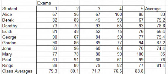
Now, that's a perfectly lucid and serviceable read on the data, complete with an alphabetical sort of student names. But with a bit of formatting derring-do and a jot of number-crunching savvy, you could come up with something like Figure 1-4:

Figure 1.4. The same grades, this time formattted to highlight the highest grade in each exam. Each set of student grades is also charted.

What additional information does the revised gradebook provide? Well for one thing, it singles out the highest student score on each test, backgrounding that score with a reddish tint (note the shared top honors in tests 1 and 2; the color choice is your call). For another, our new and improved gradebook tacks on a mini-chart called a Sparkline alongside each student's average, capturing her trajectory of test performance—a rather cool feature that's not exactly new, but which is new to Excel 2010. (Note Mary's steady upward performance slope, for example.)

Now imagine these features applied to the gradebook for a class of, say, 200 students, and note the ease with which you could identify top scorers, and how cogently those 200 Sparklines could delineate each student's progress. And Excel isn't afraid of big numbers, either; think about a university registrar using Excel to compile the course grades of, say, 20,000 students, each one treated to his own Sparkline. Why not? It's a striking way to deliver the big picture in fine-grained form.

Now, are the spreadsheet skills I've applied to these examples the kinds of things you can learn right away? Well, maybe not right away; but with a modicum of determination and reflection and some concerted practice time, the skills begin to build. After all, everyone starts at square one.

Excel is a vast application, and there's always more to learn about it. There's a batch of features you have to know in order to be able to use Excel productively; there's also a large trove of features that are very nice to know, but not quite as indispensible. No one expects you to learn all there is to know about the software, and your spreadsheet needs might be rather unprepossessing, after all. I know you can keep a secret, and so I may as well confess in the interests of transparency that I've never calculated a right-tailed student's t-distribution with Excel. But the tool for doing so is there, however, and somebody out there is using it. On the other hand, I have used other built-in formulas (called functions) named INDIRECT, RANDBETWEEN, and SMALL, and a raft of others that might actually help you do the work you need to do—even if you don't realize it yet.

This book will strive diligently to introduce and explain the have-to-knows and many of the nice-to-knows, too—but all the while keep in mind that, in the matter of spreadsheets, more really is better. Know more about Excel, and your ability to add value to your data analysis will burgeon.

This is an important point. Learning more about Excel imparts a different kind of empowerment from the sort you'll experience by mastering, say, Microsoft Word. In the latter case, expertise generally serves a greater task—the business of writing and communicating. Knowing how to fashion a table of contents may be a very good thing indeed, and it's something you might need to know; still, that bit of technical wisdom won't help turn you into John Updike. But learn how to batch up a pivot table (and that's what we used to re-present the budget data you see above) and your central spreadsheet mission—portraying and interpreting your data in intelligible and informative ways—will be enhanced.

So let's begin to describe what you'll see once you actually fire up Excel 2010. Turn on the ignition and you'll be brought to a broad expanse of white space, bordered by a sash of buttons, shown in Figure 1-5

Figure 1.5. The Excel worksheet, featuring the buttons on the Home ribbon

Now, if you're a somewhat experienced Excel user—or particularly if you're an experienced user—you may find the above tableau a bit disconcerting, depending on the version of Excel you've been using to date. That's because, starting with Excel 2007, the program's interface underwent a rather dramatic overhaul, one which called for a measure of unlearning on the part of veteran users in order for them to get reoriented to the new regime (and, in a real sense then, beginners may be operating at something of an advantage, since there's nothing for them to unlearn).

Practiced users of the 2003 and prior releases had to, or will eventually have to, wean themselves off this familiar command setup, seen in Figure 1-6:

Figure 1.6. The older Excel menu bar/toolbar interface

This now-venerable interface started users off with a row of commands on top (the menu bar) and two tiers of buttons tucked immediately beneath them, called the Standard and Formatting toolbars respectively. As many of you know, clicking any of the named commands on the menu bar unfurled a drop-down menu that sported a column of additional commands, e.g., Figure 1-7:

Figure 1.7. A traditional Excel drop-down menu

And the toolbar buttons? Nuances aside, they basically supplied an alternative means for accessing the same commands inlaid in those drop-down menus. For example, in order to begin the process of opening a file you could have clicked File

Figure 1.8. The traditional Excel Open file button

which would have done the same thing. Again, the commands on the menu bar were more or less emulated by the toolbar buttons, giving users two ways of bringing about whatever it was they wanted to do. (In fact, there were and are often more than two ways, because a welter of keyboard equivalents for these commands were and are likewise available; but we're confining our introduction to the commands you'd actually be viewing onscreen).

Because this command structure remained in place for years in the Office programs, users learned it and grew at home with it. But according to Microsoft's own literature, there were problems. As new command options proliferated across successive Excel releases, and as these were assigned their places on the drop-downs and/or toolbar buttons, the job of actually finding commands became rather a burdensome task—in part because a lengthy array of additional toolbars also lay in waiting in the background, to be ushered onscreen at the user's discretion.

And there was another problem, one I've encountered more than once in the course of my instructional stints. Some newcomers to the older Office programs assumed, understandably, that the menu bar commands—again, those topmost names such as File, Edit, View, etc., you see on the upper tier—were merely captions describing the toolbar buttons nestled immediately below them. But they aren't. And so Microsoft decided that a rethink was in order.

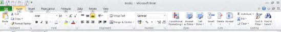
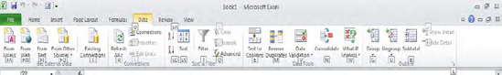
The result was embodied in a new interface that first made itself known to users with release 2007, and with it came a new vocabulary: Tabs, Ribbons, Groups, and the Quick Access toolbar. Tabs are the headings, eight by default, that hold down the upper part of the interface, and that bear a genetic resemblance to the nine menu bar command headings topping the older interface. Indeed four Tab names—File, Insert, Data, and View—reproduce four menu bar names, as shown in Figure 1-9:

Figure 1.9. The new-look tabs

And what do the tabs do? With the exception of the green-hued File, each tab, when clicked, sports a collection of buttons that are more-or-less coordinated around a general spreadsheet objective (what the buttons actually do will be detailed in the later chapters). The Home tab, for example, the one whose contents are automatically displayed when you enter Excel, comprises a collection of buttons that in very large (but not exclusive) measure reprise buttons you'll see on the old Standard and Formatting toolbars in previous Excel releases. Buttons that help you change the appearance and position of text and numbers, and that copy and paste data—all staples of those two earlier toolbars—appear here.

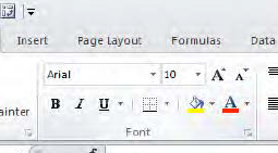
Moreover, the contents of each tab are further organized into titled groups, clusters of buttons which are even more closely themed, for example, the Font group within the Home tab is shown in Figure 1-10:

Figure 1.10. The Font button group

Users need to keep this basic understanding in mind: tabs contain groups.

Note that some group buttons are embellished with a small, downward-pointing arrow, but others are not. Click those arrows and you'll be brought to another set of related command options—ones associated with the original button. For example, click the down arrow attached to the Sort command and you'll see Figure 1-11:

Figure 1.11. The Sort command drop-down menu

This list presents you with a set of options for sorting columns of data. These arrow-driven commands are perhaps the closest thing you'll see to drop-down menus in release 2010.

Click a button with no arrow alongside it, on the other hand, and its action is often carried out on the spreadsheet immediately. Alternatively, click an arrowless button and you'll be presented with a dialog box requiring additional user action—but without the kind of sub-menu shown in Figure 1-11. Click the B button you see above in the Font group, for example—there's no arrow there—and any data you've selected on the spreadsheet acquires a boldfaced appearance right away, with no additional options from which to choose. Note as well that if you simply roll the mouse over any command on the ribbon, a small but helpful description of what that command does, called a tooltip, materializes.

Another point about tabs. By double-clicking any tab you can submerge, or minimize, the buttons populating the tabs in order to streamline the appearance of the top of your worksheet, as seen in Figure 1-12:

Figure 1.12. The 2010 tabs, after having minimized the button groups

(You actually need to double-click a tab twice to achieve this effect. The first double-click takes you to the button contents of the tab on which you've clicked; the second double-click minimizes all the buttons.) Double-clicking any tab heading returns all the buttons to view (you can also minimize by right-clicking anywhere among the tab names and selecting Minimize the Ribbon on the resulting dropdown menu. You can also minimize the ribbon by clicking the caret-like up arrow in the upper far-right of the screen, right above the ribbon. Clicking that arrow a second then restores the ribbon to view.

In addition, some—but not all—of the groups populating the tabs feature a small, right-pointing arrow in their lower right corner, revealingly called the dialog box launcher, see Figure 1-13:

Figure 1.13. Where to find the dialog box launcher

If you simply rest your mouse atop one of these arrows without clicking yet, a small description of what's going to happen after you do click bobs to the spreadsheet surface. In the case of our group above, the description states, "Shows the Font Tab of the Format Cells dialog box" (along with a keyboard equivalent of the command you're about to execute). Go ahead and click, and you'll call up this object shown in Figure 1-14:

Figure 1.14. The Format Cells dialog box

Look familiar? If you've used any of Excel's pre-2007 releases, it should. What's you're seeing is the good old Format Cells dialog box, the same object that would have made its way onto your screen via the menu bar command/drop-down-menu sequence in the older versions. This dialog box, and others like it that have seeped into the 2010 interface, make a retro visit to the predecessors of Excel 2010, as if to afford discombobulated users a friendly, tried-and-true alternative to all those newfangled tabs and groups they're faced with now.

And this continuity—the availability of dialog boxes from earlier Excel generations—divulges a kind of open secret about Excel 2010 to users of the pre-2007 era: Once you drill down beneath the Tab-Group interface and reach the commands that actually make something happen on the spreadsheet, you'll find that many—though certainly not all-of these commands, particularly those in dialog boxes, are virtual replicas of earlier ones. The fact is that much of the DNA of earlier Excel generations has been encoded into 2010, pointing us to the conclusion that Excel 2010 isn't quite the radical break with the past you may first take it to be. The wheel hasn't been completely reinvented, even if the hubcap has been restyled.

On the other hand, even if you're coming to Excel 2010 from the 2007 rendition, you'll quickly observe one significant departure from that latter interface—the debut of the File tab, distinguished from all the other tabs by its conspicuous green cast. The File tab supplants the 2007 Office button—perhaps destined to go down as a one-hit wonder, having come and gone with that release alone (See Figure 1-15.)

Figure 1.15. The Office 2007 button

The suspicion was that too many users mistook this button for nothing more than an inert logo when they first saw it, and not as the repository of important commands it actually was (my wife, a moderately experienced user, tells me it took her ages to figure out what the button did). In any case, click the 2010 File tab and this time you won't roll out one more array of buttons atop your screen; instead, you'll see something like Figure 1-16:

Figure 1.16. All buttoned up: How the 2010 File menu looks

Clicking File, the rough—very rough—equivalent of the pre-2007 menu bar command with the same name can bring you to a number of notable destinations gathered in what's called the Backstage:

And File allows you to customize your ribbon in a variety of ways, either by enabling you to fashion new groups you can then post inside the existing tabs (quick review: groups are the subdivisions of tabs) or freeing you to customize new tabs altogether, by selecting, grouping, and subsuming commands under a new tab name of your devising.

That last point also reminds us that Excel is stocked with a rather prodigious array of commands that, by default, don't appear on any tab. But they're all listed here in the deeper recesses of File, to be added to tabs by users who need them, as shown in Figure 1-17:

Figure 1.17. Inside the File tab, where all of Excel commands are listed

Figure 1-17 captures but an excerpt of all the available commands; and while you may not need to import too many of these into your tabs, remember the knowing-more-is-better credo. There are some cool capabilities stored in that list—capabilities you may one day decide you'd like to use.

All of which segues into the Quick Access Toolbar (QAT), a rather mild-mannered strip of buttons you'll find lining the upper-left perimeter of your Excel screen, as seen in Figure 1-18

Figure 1.18. The Quick Access toolbar

Apart from demonstrating Excel's tenacious attachment to the word "toolbar," the QAT plays a valuable role in enabling you to access important commands easily. Stocked with but three buttons at the outset—the ones which execute the Save, Undo, and Redo commands—the QAT can be tailored to store any other command buttons—ones you presumably want to use often. The idea is that you can post any existing, tab/group-based command to the QAT so that the command remains available even when you go ahead and move on to a different tab.

For example, suppose you're a pivot table devotee, and while you know that the command for designing a new table is housed in the Tables group of the Insert tab, you want to able to activate a pivot table at any time—even if you now find yourself in, say, the Data tab. By right-clicking your mouse on the Pivot Table command (important note: unless otherwise indicated, all mouse clicks in this book call upon the left button) and clicking the Add to Quick Access Toolbar option shown in Figure 1-19

Figure 1.19. Where to add commands to the QAT

you can dispatch a copy of the Pivot Table command to the QAT, where it makes itself available whenever you want it (Figure 1-20 ):

Figure 1.20. QAT access to the Pivot Table command

No need to revisit the Data tab; just click Pivot Tables on the QAT instead—and there's your pivot table.

You can also install any command onto the QAT from that master list of all Excel commands catalogued in the File tab.

Now there's one more component of the 2010 interface you'll want to know about, one which appears only on occasion. When you add certain elements to your spreadsheet—e.g., one of those pivot tables, or a chart, or a Sparkline, or a graphic object (say, a shape or a picture), and return to that object and click on it, a command name alluding to that object suddenly pokes its head atop your screen. What does that mean? Well, let's return to our grading sheet, complete with those student-performance Sparklines. Click on any cell containing a Sparkline, and you'll trigger this display (Figure 1-21):

Figure 1.21. The Sparkline Tools tab

Click that amber title (the color varies by whatever object you're working with) and a new set of tab contents barges onscreen, overriding the tab with which you'd been working to date. What you see now instead is a battery of options devoted to Sparklines alone (Figure 1-22):

Figure 1.22. Sparkline tool buttons

Complete your Sparkline revisions, click on any other, non-Sparkline-bearing cell, and this tab disappears, returning you to the previous tab. Whenever you click any Sparkline cell, that tab revisits the screen (again, how Sparklines actually work is to be taken up in a later chapter). Thus these object-specific, now-you-see-them-now-you-don't tabs give you swift access to the commands for working with some special spreadsheet tools—exactly when you need them.

Now let's add an important navigational note to the proceedings. We've spent a good deal of time in the company of our trusty mice, ambling across the 2010 interface with those redoubtable pointing devices leading the way. But there's also a keyboard-based means for accessing all of the above elements:

Tap the Alt key, and these lettered or numbered indicators suddenly attach to the tab headings and the QAT (Figure 1-23):

Figure 1.23. Alt keyboard options

Then tap any one of the letters/numbers you see called Key Tips (this time without Alt), and that tab's contents display. Thus if you tap A as we see it here, the Data tab's buttons will appear, each command of which is then also lettered. Then tap any one of these letters (and note some commands comprise two letters—these should be tapped rapidly in sequence), and the command executes, as shown in Figure 1-24:

Figure 1.24. Inside the Data tab: Alt key options

Thus if I type SD now, a selected range will be sorted in descending alphabetical order (and don't worry what that means if you aren't sure. Sorting is to be explained later. But note that SD = Sort Descending). And once the command does its thing, all the letters disappear. And if you initiate the whole process by tapping Alt and then have second thoughts about it, simply tap Alt a second time, and the letters vanish—no harm done. Thus the Alt approach offers one more way of getting the same jobs done—but this time with no mouse required, if you're so inclined. Commit a few of these Alt-ernatives to memory and you should be able to speed some of your basic, recurring tasks as a result (and just for the record—the Alt technique in subtler form also works in the pre-2007 releases of Excel, too).

A couple of other points before we wind up. The way in which the ribbon's contents appear on your screen will depend in part on your screen's resolution (I speak from experience). Your button captions may thus be positioned differently from ours, and so the screen shots in this book may not precisely correspond to what you're seeing. So rest assured: you're not hallucinating, you just have a different screen setting. And here's something else that you won't see in previous Excel versions: when you select text (defined broadly, here, as including numbers as well)—that is, when you actually highlight the text, as opposed to simply clicking on a cell—you'll see a dim, apparition-like toolbar looming a bit above the cell. Lift your mouse just a bit, and the toolbar—called a mini-toolbar—resolves sharply on screen, as shown in Figure 1-25:

Figure 1.25. The mini-toolbar

The mini-toolbar supplies you with speedy access to standard text formatting option buttons — bold, italics, etc. Click one and the change is made. If, on the other hand, you find this utility literally gets in the way, you can turn it off by clicking File

We can begin to figure out how to pour our data into that massive space—and make the data work for us.

So let's begin.