
Stop me if you've heard this one before: An efficiency expert intercepts a 911 call from a desperate boss, begging her to drop everything, don her flak jacket and sensible shoes, and zoom over now to do something about his workplace, overrun to the breaking point with unstoppable, rectangular blobs of paper. Throwing caution to the winds, our fearless expert pokes through the debris, and after skidding on a couple of 8½ × 11s and running her paper cuts under the water cooler, finally doffs her helmet and announces hopefully: "It's really very simple: All you need to do is just scan all these hard copies, and burn them onto a couple of CDs; in a few hours you'll be able to see your floor again."
"Great idea!" exults the grateful boss. "But just one thing: before I start scanning, let me make some Xeroxes for backup..."
Paperless office? Probably not your office, and probably not your home, either. They still make Excel with the Print command, and sooner or later you're going to have to beam that digital doc to your local neighborhood output device and turn it into something you can actually hold in your hand and spill coffee on. It's retro, but true; you need to know how to print, and when you do, Excel makes it pretty easy to navigate the transition from software to hard copy.
The first thing to understand about Excel printing is to know exactly how much of the workbook you want to print. By default—that is, if you work with the initial print settings supplied by Excel—carrying out the print command will print the entire worksheet (but not the entire workbook). And by the entire worksheet, Excel means all the cells in the sheet containing data. And that means in turn that, if you want to print the cells spanning A3:B20 and you've also squirreled a clandestine value in cell X4578, Excel will print 258 pages or thereabouts. That's because when it goes ahead with those default print settings Excel prints all the empty space between the data-bearing cells in addition to those cells you really want to print; it preserves the relation in space between all the cells from A3:B20 through X4578. As a result, I'll print 256 empty sheets in addition to the two that contain my values.
Of course, that's an extreme—but not unprecedented—scenario. Worksheets can be teeming with data, and even if those data are confined to one particular area of the worksheet—say, to a 20,000-row table, of which you want to print just 500—going with the default print settings will get you 20,000 rows worth of paper.
Needless to say, Excel is happy to let you overrule its defaults, but it's time we tried this all out. Let's call up the Sales by Year spreadsheet, and click on the 2010 tab, containing that small range of sales data for that year. Let's say we want to print the entire sheet, at least for starters. To start printing (after you'd made sure you're duly connected to a printer, and that it's turned on), you can click the File tab

Note first of all the Print Preview occupying the right half of the screen. The desired print range is captured, and all the default settings remain in place at the outset. To review the settings:
The Copies option is pretty self-evident. If you need to print multiple copies, just type the copy total or click up the spin control arrow.
Printer designates the printer that will output the copies. Because you may have access to more than one printer, you may have to click this option's drop-down arrow and select the appropriate device. Among the "devices" you may see a Print to PDF option—not really a bit of hardware but the widely-used document format, through which an Excel workbook can be read by users who don't have Excel. By selecting this option you'll "print" a PDF file to your computer. And if you need to identify your printer for the first time, the Printer command's Add Printer... options lets you start that process.)
The Settings area features a number of important fields, its options presented in drop-down menus. Print Active Sheets serves as the default in the first of these, and when selected prints all the data in the active sheets. But why the plural—why sheets? That possibility refers to sheets which may have been grouped, and if you have grouped multiple sheets, the data on all of them will be printed, and on separate pages—at least by default. Continuing with the field's other options: Print Entire Workbook will print all the data on all the sheets of the workbook, each worksheet assigned its own print page. Of course, if the data on any one worksheet is extensive, that sheet may require a multi-page printout in its own right. Print Selection, sub-captioned Only print the current selection, lets you select a range on the sheet and designate just that range for print output. Thus if you select 500 of the 20,000 rows in the table we cited earlier, only the 500 will print—and you'll see evidence to that effect in the Print Preview (note that a multi-page Print Preview lets you click to each page via the arrows at the bottom of the screen). However, if you click in a table, a new option presents itself in the drop-down menu—Print Selected Table. Click it, and just the table prints.
The final option in this field—Ignore Print Area—requires a bit of a digression. We've already seen how the Print Selection command works, but you can also select a range of cells before you click the Print command and then click the Page Layout tab
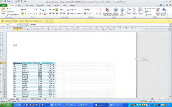
To illustrate this option, open the SampleSalesPerson report on which we tried out our pivot tables. Click if necessary on the Source Data tab at the bottom, and select cells A1:E50. Then click Page Layout

Note the selected print area we've established—A1:E50—appears in the preview. Then click Ignore Print Area, and you'll see (Figure 9-3):

Note the page count at the bottom of the page: 14. That means if we launched a printout right now Excel would print the entire table, because we've temporarily overridden the A1:E50 print range and returned to the Print Active Sheets default, as it's shown in the Backstage. Then by clicking Ignore Print Area off, we'll return to the A1:E50 selection. And you can turn your Print Area off permanently by clicking Page Layout
The Pages option enables you to indicate which pages you want printed, in the event your selected print range—or the entire active sheet - spans more than one page. Note by default the page number fields are blank. By clicking the horizontal arrows at the bottom of the page you can view how your data appear before selecting your pages. What this means is that if you select some, but not all, of the pages to print you're really carrying out a kind of alternative Print Selection command. Note as well that, unlike Word, you can't print non-consecutive pages in Excel.
The Collated options really only apply to multi-page, multi-copy printouts and work very similarly to the way in which they work in Word. By default, Excel collates by printing copies separately in their page sequence. Thus if we were to print three copies of the entire Source Data sheet in the SampleSalesPerson workbook, we'd roll out all 14 pages, 1-14, three times. The Uncollated (another Un word—even Word redlines it) option, however, prints all the page ones, twos, threes, etc. together in that sequence. Printing the Source Data sheet in Uncollated fashion would yield three page ones, three page twos, etc. And why would one want to print this way? Perhaps because a lecturer who needed to enter some handwritten corrections on all the page ones, for example, could more easily grab every copy of that particular page via an Uncollated printout.
Portrait Orientation is Excel's default print orientation. That is, leave this option as is and your printout will appear in a vertical, upright position. Your print needs may often require a landscape, or sideways orientation, though, and if that's the case simply click the Landscape orientation. Either way, the Print Preview will display the pages in the selected orientation. (Note: You can also access the Orientation option by clicking the Printer Properties link beneath the Printer drop-down menu, as well as by clicking the Page Layout tab

The Letter drop-down menu provides a series of paper sizes you can select for your print. Naturally, the standard 8½ × 11 size appears by default (or A4 if you're on the other side of the pond), but the associated drop-down menu stocks a long list of additional options. And if those aren't enough, clicking the More Paper Sizes... selection calls up the ageless Page Setup dialog box (Figure 9-4):

Click its Paper Size down arrow and still more possibilities materialize. You can even print to an index card, or a Japanese postcard. We'll have more to say about Page Setup later.
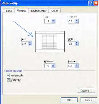
The Margins option lets you adjust this print dimension. We generally don't think of spreadsheet margins in the same terms we ascribe to word processing, where they play an essential role. As a rule we don't trouble ourselves with Excel margins, because working electronically on formulas and tables doesn't require a uniform layout, at least not usually. But a printout is a printout, and you have no choice but to consider its margins once you put toner to paper. By default, Excel starts you off with margins of .7 inches left/right, and .75 inches top/bottom—what it calls Normal Margins (the Headers options will be discussed soon), but you can obviously change these as you wish. Click the drop-down arrow by the Margins option and you'll be brought to two additional built-in recommendations, Wide and Narrow. The former suggests measures of 1 inch in both directions, while Narrow offers a top/bottom of .75 inches, and .25 inches left/right. Not happy with any of these? Click the Custom Margins... option, and you'll be returned to the Page Setup dialog box, this time its Margins tab (Figure 9-5):

Page Setup allows you to type or click margins of your own choosing, and also introduces a different and useful option as well—Center on Page, which enables you to center a print range horizontally across a page, and/or vertically over the length of the page. Select both possibilities and your printout winds up smack-dab in the middle of a page. Note the change in position of the sample image when I click both centering options (Figure 9-6):
(Note: The Page Setup dialog can also be accessed by clicking the Page Setup link at the bottom of the Print dialog box, as well as by clicking the dialog box launcher in the Page Setup button group on the Page Layout tab.)
The final option in the Settings group in the Print menu controls Scaling (sounds like a hair shampoo). By default, Excel prints sheets "at their actual size," a rather ambiguous instruction that means that the printout will emerge as it initially looks in the Print Preview. But you can modify that hard copy outcome, and there may be good reasons to want to do so. Note these drop-down scaling options (Figure 9-7):
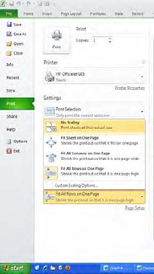
Moving past the No Scaling default we're brought to the Fit Sheet on One Page option, an important one that addresses a classic spreadsheet print challenge: how to deal with a worksheet whose contents when printed will spill onto a second page—barely, by just a few rows or so. Printing here with No Scaling will yield an unsightly Page Two, consisting of but that smattering of data. Click Fit Sheet on One Page however, and all the worksheet data will be ever-so-slightly-downsized, all amicably sharing one, smartly presented page.
Of course, Fit Sheet on One Page needs to be used with care. I once accidently printed a lengthy worksheet under that option, and the one-page result looked like raw seismographic data, or someone's EKG readout. Ah, well...we learn from our mistakes.
The other two drop-down options—Fit All Columns on One Page and Fit All Rows on One Page—address related print issues. If your printout as engineered by the No Scaling mode results in one lonely column being elbowed onto a second page, that's not going to look very nice—but we need to figure out what's really going on here. The printout in question could in fact be dozens of pages long—because, for example, you may have to print a couple of thousand rows of data—and so we're not dealing with the one-versus-two page spillover problem we described earlier in the Fit Sheet on One Page discussion. Here the issue is one of print width versus print length. We're prepared to roll out dozens of pages worth of table rows—but we still want the table fields, or columns, to all appear on every page of the printout, and it's this print objective that Fit All Columns on One Page carries off. Thus if you have 50 pages worth of table rows streaming down the pages vertically, so be it—but if one table column also spills over onto a second page horizontally, you'll wind up with a 100-page printout, because every row needs to display its data beneath that excess column, too. And that's downright gauche—but it doesn't have to happen, unless you have dozens of table fields to work with, and fitting them all horizontally on one page crunches the data into text best viewed under an electron microscope.
The companion option—Fit all Rows on One Page—resolves the same sort of print issue, but in a perpendicular direction. If you want to print a table say, three columns wide by 50 rows high, it's possible that a row or two will creep onto a second page, depending on your current margins, row heights, and the like. Use Fit all Rows to reel those truant rows back onto one, all-encompassing page.
But note that the Scaling drop-down menu also sneaks in the Custom Scaling Options... selection, which when clicked opens the stalwart Page Setup dialog box, treating you to a couple of additional scaling possibilities (Figure 9-8):
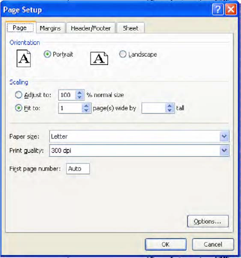
Adjust to lets you modulate the size of the printout by a percent of the original, "actual" print size. It thus affords you a way to enlarge a small print range so that it occupies more of the page if you type a percentage greater than 100. On the other hand, entering a percentage less than 100 can act as a variation on the Fit Sheet on Sheet One Page option. Type say, 92 in the Adjust to field and you may be able to make room on page 1 for those few excess rows that have tip-toed onto page 2.
Fit to represents a variation on the Fit All Columns or Rows On One Page options. It lets you resize the printout either horizontally or vertically, and again may come into play if your printout experiences a small surplus of columns or rows. If, say, the last five of the 200 rows you want to print get bumped onto a new page—say page 4—you can click 3 in the tall Fit to field, and Excel will shrink the row sizes just a bit in order to achieve a three-page-tall output, which now encompasses all 200 rows. These options are also available via the Page Layout tab
It may not be something that immediately comes to mind to Excel users, but you can add header and footer information to your prints, so that a recurring bit of information—such as today's date, the current page number, or your workbook title—will appear at the top and/or bottom of your pages. There are two rather different routes to headers and footers, and we'll start with the original, classic approach.
The basic tools for adding headers and tooters are stored in the Page Setup dialog box, which, as stated earlier, can be accessed in several different ways. To demonstrate, let's open the SampleSalespesonReport workbook, if you haven't already done so. Select cells A1:E100, and set the print area via the Page Layout tab
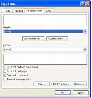
This dialog box, little changed from previous Excel versions, offers you a pretty extensive array of pre-packaged header/footer options. Click the down arrow by Header, for example, and you'll get (Figure 9-10):
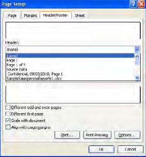
Click on the first drop-down option and your printout will display the page number at the top of each page. The next selection, Page 1 of ?, indicates the current page number relative to the total number of pages in the printout, e.g., Page 1 of 3, Page 2 of 3, etc. Source Data refers to the name of the particular worksheet on which you're working in the header, and so on; and these options are likewise available on the Footer drop-down menu.
You've also doubtless noted the Custom Header... and Custom Footer... buttons posted in the dialog box, too. These enable you to do two things that aren't available in those initial drop-down menus: They allow you to align a header or footer on the left, center, or right of a page, and they allow you to enter your own, customized text, e.g., your name, or Acme Widgets, Inc., as well. To see what I mean, click Custom Header.... You'll see (Figure 9-11):

Note the instructions contained in the dialog box as well. The buttons are more-or-less organized in groups, as you see here, surrounded by the ovals. If you want to enter your own text header, just click in the appropriate section above and start typing. To format the text, just select what you've written, click the A button, and select the font and its size. The next two buttons when clicked post page references in the form of codes—page number and number of pages in the printout, respectively. You can enter both in one section, and insert the word "of" between the codes, thus yielding 1 of 2, 2 of 2, etc. The next two buttons insert date and time codes. Time inserts an updatable current-time code, such that whenever you print the document the correct time will appear on the printout and/or Print Preview. The next three buttons will insert the file path (e.g., c:My DocumentsSampleSalespersonReport.xlsx—often used in offices, so that other employees will be able to locate the workbook), the file name, and the sheet(tab)name. The last buttons will, when clicked, let you insert a picture in the header or footer, and allow you to edit it with assorted picture tools (enabled by the very last button).
For example, if I type my company name in the left header section, enter today's date in the center (whenever that is), and the page number in the right, these selections will look like this, as Excel codes them (Figure 9-12):

Click OK and these elements will appear in your header. Needless to say, all these options can be applied to footers as well. You can easily see how it all looks by clicking the Print Preview button in the Page Setup dialog box, or even by just viewing the small preview screens in the Page Setup Header/Footer tab.
You'll also note four check box options on the Header/Footer tab. Different odd and even pages lets you supply different headers and/or footers for odd and even pages. By checking that box and then clicking Custom Header or Footer, you're brought to a slightly changed dialog box (Figure 9-13):

Note the tab names, easy to overlook, but now changed; and what they do is pretty self-evident: click Odd Page Header and any header elements placed here will only appear on the odd pages of the printout - and you can guess what Even Page Header does.
Different first page likewise pulls no surprises, enabling you to treat the first page header/footer differently from the remainder of the printout - an option that includes imparting no header/footer to page one, even as the other pages show them. Check that box and then click Custom Header, and you'll see at the top of the dialog box (Figure 9-14):

By now you know how this works. While this is the kind of option you'd expect to see in Word, and you do, First Page Header may have a place in Excel printouts too. You may want to see a date on page one alone, for example.
The next two check-box options are turned on by default. Scale with document changes the size of header/footer text in line with the rest of the worksheet if you resize the sheet. Clearing the option preserves that text size even if you do make a print-size change. Align with page margins moves the header/footer along the page horizontally (but not vertically, even if you change the top/bottom margins) if you change the left and/or right margins. Turning off the default keeps the header/footer in place, even if the margins do change. Thus if I post a page number header in the left section of SampleSalespersonReport as per the default, Normal margins, I'll see (Figure 9-15):

But if I change the left margin to 3 inches and leave Align with page margins selected, I'll see (Figure 9-16):

The entire printout, including the header, has moved to the right.
Note as well that the Margins tab allows you to select the position of headers and footers relative to the physical top and bottom of the printed page (Figure 9-17):

Remember that the values you choose here enable you to reposition the header and/or footer relative to the physical edges of the page, and is independent of any Top/Bottom margin changes. Thus ratcheting the Top margin up to 3 won't automatically push the Header distance down along with it.
Time for another classic, and related, print problem: you want to print a lengthy table, which is as usual topped by a header row (not the headers we've just discussed, but rather, the first row of the table). Once the printout reaches page two, the header row is nowhere to be seen. Because it's the very first row in the table, the header row is naturally going to make its appearance on page one—and only page one. But you want all the pages to show the header row on top, so that a viewer of the printout can always clearly tell which data belong beneath which field. The way to carry this off is with the Sheet tab in the all-purpose Page Setup dialog box. Note that our SampleSalespersonReport illustrates this problem: Click anywhere in that report and turn to the Print Preview (all you need do is click Ctrl-P), then click the horizontal page-scroll arrow at the bottom of the screen to page 2. You'll see (Figure 9-18):

You see the problem. The reader can't easily determine how the respective data are labeled on page two, because the header row just isn't there. By clicking the Page Layout tab
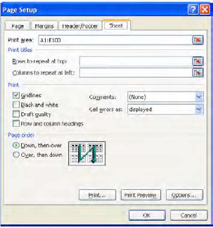
Click in the Rows to Repeat at Top field, and then click anywhere on row one in the worksheet. You'll see Figure 9-20:

That selection guarantees that the contents of row one—which contains the table header row—will appear at the top of every printed page, even if the print is 100 pages long. Now page two of our salesperson report looks like this (Figure 9-21):

The header row has been instated here as well, insuring a much more readable report. You can also select the Columns to repeat at left option, which will allow a column or columns to likewise appear on every print page on the left of the page. Thus if you have a column of months in the leftmost column of a wide, multi-columned worksheet and you need to see those months on every print page, click anywhere in the month column and it will appear on every sheet. (Note: This option is only available via the Page Layout tab
The Sheet tab also contains a few other options you may want to know about. The Print section there lists a quartet of check box items, starting with Gridlines. Checking this will enable you to print the gridlines that you see traced around every cell (at least by default) on the worksheet. This is an all-or-nothing command, however, meaning that any empty cell you've included in a print range will also sport gridlines in the printout. (As a result, you may want to use one of the Border options in the Font button group on the Home tab instead, in order to draw lines around only the cells you want.) Black and White will output your worksheet in those famously binary colors, even if you're working with a color printer, the better to save color toner. Draft quality is another economical print option, instructing your printer to roll out your worksheet at a lower print resolution—assuming your device is capable of varying its print quality in this way.
Row and column headings is a selection you see utilized now and then, enabling you to actually print the alphabetical and numeric column and row borders of the worksheet. Avail yourself of this option and your print will look something like this (Figure 9-22):

This option might prove instructive to readers who want to visually line up the data in their cell addresses.
And moving down a bit on the Sheet tab you'll see Page Order, an option that comes into play for unusually long and wide printouts. If you need to print a large number of columns and rows you may wind up printing pages in both directions—that is, pages that print the rows downward across the width of the page, but also another set of pages that print the "excess" columns spilling across horizontally, containing the row data sitting beneath those columns. By default, Excel will print data Down, then over, meaning that if your print area is say, 20 columns wide by 500 rows high, the printout will first print "downwards", until all 500 rows are printed with as many columns as can be accommodated on those pages, and then will print the remaining columns streaming across the extra pages—those columns and row data that couldn't fit on the first set of pages. Select Over, then down, and the printout will print everything "across"—that is, all 20 columns across the first two pages, with as many rows beneath them as can be fit, and then another 20 columns across, with the next batch of rows, etc.
Open a worksheet and by default its contents flash onscreen in what's called the Normal view. But Excel makes alternative views of the worksheet available, too, and there are reasons for wanting to switch to them, at least on occasion. In fact, we've already worked with one such alternative—the Print Preview—throughout this chapter. But other viewing options are out there, too, among these the Page Layout view, available in a button bearing that name in the View Tab

This view really is different in some important ways. The worksheet column and row headings remain visible in this view, but they're separated from the page, to indicate that they won't be printing by default (but if you do elect to print the row and column headings, they'll appear twice in this view—on the margins, as you see in our screen shot, but also on the worksheet proper). Note in addition the ruler, which allows you to determine how much space on the printed sheet each row and column will occupy. Moreover, you can see that Page Layout delineates the contours of the paper page, showing where the edge of a sheet gives way to the next sheet.
It's also important to understand that the Page Layout view is live—that is, you can actually enter data while working in it. You'll note the Click to Add Data prompt on the far right of the screen shot above, a slightly misleading instruction because it implies you can only enter data there. Not true; you can work as usual in any cell on the worksheet here, including those cells that already contain data. Just remember that by entering information in the Click to Add Data area you're including those data in your default print range. Note as well that if you guide your mouse into the narrow gray corridor between pages in the Page Layout view, you'll encounter a Hide White Space caption(Figure 9-24):
Click there and the header/footer areas on the worksheet—that extensive white space—will be banished from the screen, leaving you with more of the worksheet proper on which to work. Slide back into that sliver again between the pages and you'll see a Show White Space prompt; click there to expose the header/footer areas.
Any print range you've set will continue to be bordered by a dotted line in the Page Layout view. Recall that we've established A1:E100 as that range, an area of cells that should yield a two-page print. But—and this is easy to miss—check out the left edge of the status bar in our screen shot (Figure 9-25):
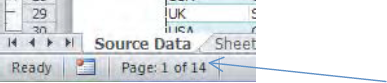
This looks like the sort of message you'd see in Word, but in any case it raises a question: Why 14 pages? It's because Page Layout tallies the number of pages you'd get were you to print all the data in the worksheet—even though we want to print just 100 rows. And along these lines, note that Page Layout continues to display the filter buttons on the table's header row—but these won't print.
You've also probably caught the Click to add header area (of course there's a parallel Click to add footer section here, too); but before you actually click, roll your mouse over there and note that the header area turns blue over whichever of the three header sections you're rolling—that is, the left, center, and right sections that emulate the sections we saw in the Custom Header/Footer option in Page Setup (Figure 9-26):

Once you've clicked here a Header & Footer Tools tab tops the screen (Figure 9-27):

Figure 9.27. More of the same: Buttons in the Header & Footer tab, duplicating the options in the Page Setup dialog box
This tab contains what are really the same custom header/footer options we viewed in the Page Setup dialog box. Click any Header & Footer Element button (no, I can't explain Excel's fondness for the ampersand here instead of the word "and") and you can add a page number, date, file path, etc., just as you can via Page Setup. And if you want to add your own text-based header, just type it after you've clicked in a section (Figure 9-28):

When you set a print area for a multi-page printout of the worksheet, Excel will naturally occupy the entire first page with data and then move on to page two when it runs out of space, and so on across all the printed pages. But sometimes you want a next page to start with a particular row on top, for the sake of appearances—but Excel can't know that, at least not by default (Note: We're not referring to the rows-to-repeat-on-top issue here. Here we want the row to appear just once, but at the top of a specific printed page.) You can, however, instruct Excel to relocate the point at which a page breaks—at least within limits, with the Page Break Preview option. By clicking the View tab
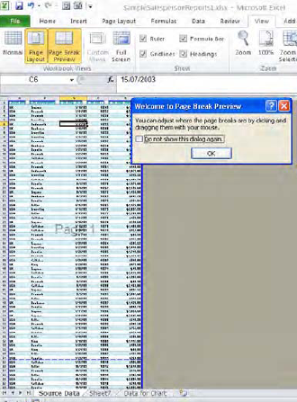
This is an old Excel option, with a curiously shrunken image of the worksheet (to enable you to get a bird's eye view of the print breaks) and a quaint dialog box to boot (I mean, how many of them start with "Welcome to..."?). Click OK, and you can then begin to adjust your page break settings.
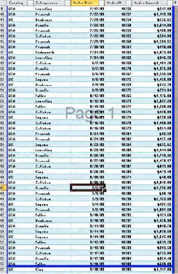
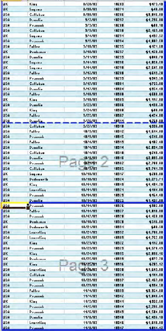
The dotted line you see above at row 61 represents the current point at which Page 1 breaks (note the watermark reference to the page number), and if you click on that line and drag it either upwards or downwards, you'll be able to move the page break point to a different row. (If you drag downwards, you'll naturally be adding rows to the page—requiring Excel to rescale the page downwards in order to accommodate those rows in view of the existing print margins. There's only so much physical space on the page!) Drag, say to row 56, release the mouse, and you'll see (Figure 9-30):
The dotted line page boundary has been replaced by an unbroken line, indicating that the break has been introduced by the user, not by Excel. And because we've lifted the page break on Page 1 by five rows, establishing the break five rows "earlier" on the page, Page 2 will now break five rows earlier, and so on.
And while it's easy to miss, you can click and drag on the vertical boundary of a print range and widen the range by adding columns to it, or narrow the print by excluding columns you had originally earmarked (Figure 9-31):

Note again that, as with the Page Layout view, the Page Break Preview is live, allowing you to enter data in this viewing mode, too—though the text appears so small that typing may pose a challenge (Note: By clicking the View tab
Now there's another, closely related option to the Page Break Preview stored in the Page Layout tab

Is that what you had in mind? Maybe—but maybe not. Clicking in cell D77 and clicking Breaks does what it told you it would do—it institutes a page break above D77, but also another one to the left of that cell, resulting in more pages in all directions. If all you really wanted was one more page running down the printout, you'd have clicked in A77, or the 77 row header instead, and then clicked Breaks, yielding this Print Preview (Figure 9-33):
But not to worry. If you've introduced page breaks in all the wrong places, you can click Page Layout
You can also prepare a print setting complete with a set range, hidden rows and columns, and filter settings in effect (i.e., all sales over $5,000), and save all this as a CustomView, so that you can change that filter setting, etc., and go on to do other things on the worksheet. You can then trot out the View when you're ready to print, and all those saved settings return to the screen.
Note that you can't save a Custom View to a worksheet that has a defined table on it, so in order to demonstrate how this works, click in the Salesperson Report table and click the Table Tools context tab

(Remember that we've already set the print range.) Then click the Views tab

Click Add. Type "newview" in the Name field. Note that the current print settings and hidden rows, columns, and filter settings will all be saved by the View. Click OK. Then unhide column C, and click Select All in the Country filter, restoring the UK records to view. Then Click View
As we've seen, Excel is happy to supply you with a whole range (pun intended) of print options, designed to let you nail down exactly what you want to print. Still, print basics are pretty basic—select your print range, tell Excel about it, and let 'er rip. Now we're going to reverse our field—or medium—by moving from paper to the Internet, to describe how you can share and contribute to workbooks posted out there on the Web.