Let's start at square one—literally, by returning to Excel 2010's blank worksheet, which is what you'll see when you enter the program, as shown in Figure 2-1:

Figure 2.1. The 2010 worksheet, or at least part of one

And, as you scan this rather panoramic scene, we'll trot out a few more of those have-to-know concepts, ones you'll need to keep in mind in order to steer your course across all this territory spread out before you. You're looking at a worksheet—or more strictly speaking, part of a worksheet, an integral part of a workbook. A workbook, simply put, is really Excel's name for a file, the kind of object you'll find listed in My Documents, e.g., familybudget.xlsx. What Microsoft Word calls a document, then, is what Excel calls a workbook.

By default, the workbook is outfitted with three identical-looking worksheets, all of which are represented by tabs (not the kind we explored in detail last chapter) in the lower-left corner of the workbook, as shown in Figure 2-2:

Figure 2.2. Keeping tabs on the worksheets

You can supplement these three start-off worksheets with additional ones if you wish, or delete them (though you can't delete all of them, of course; otherwise you'd have nothing left), and you can even hide a worksheet. Why might you need to use several worksheets? For example, a university professor might want to assign a sheet to each of the classes she's teaching, listing each roster of students and their grades on each sheet. And for ease of data entry and review, all the sheets could be designed and formatted identically.

As you can see, the worksheet comprises an enormous grid, criss-crossed by lettered columns and numbered rows. Each intersection of a column and row is called a cell, each of which in turn bears an address, identified very simply by its unique combination of column letter and row number. Thus in Figure 2-3 the cell pointer—that thick-bordered rectangle that gallivants across the worksheet—finds itself in cell C7:

Figure 2.3. Selecting cell C7

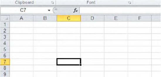
You'll note of course how the respective C column and 7 row headings have changed colors, denoting the current position of the cell pointer. A little less obvious, though, is the C7 (it's never 7C, by the way) posted in the upper left of the screen shot. As you can see, that sliver of space up there, called the name box (and why it's called the name box is to be explained a bit later) records the whereabouts of the cell pointer; and the two kinds of indicators—the column/row-heading color change and the name box cell reference—make it easy to know exactly where you've situated the cell pointer.

And as for the cell pointer itself, its position marks that point in the worksheet where data will go when you begin to type. Thus if I type the number 56 in our screenshot, it will be posted to cell C7.

And as we earlier observed, the worksheet is large—very, very large, consisting of 16,384 columns and exactly 1,048,576 rows. Do the math and you wind up with over 17 billion cells, a preposterously huge number that will likely far, far exceed any purpose you and I might bring to a workbook; and given your computer's memory allotment, you probably couldn't fill all those cells even if you wanted to. Put another way—if I wanted to view the entire worksheet at one time on my screen, I'd need a display about 800 feet wide and 1.6 miles long, give or take a football field—and try to sit with that in economy class. And remember just for the record that each worksheet in the workbook boasts another 17 billion cells—so if you need to catalogue the stars in the Milky Way, for example, you've come to the right place. Just make sure you get a RAM transplant first.

But you may be bothered by a more practical issue: since we run out of letters at the 26^th column—letter Z, that is—what do we call column 27, for starters? Answer: That column is assigned letters AA, followed by AB in column 28, etc. Sidle over to the 53^rd column and you get BA, and so on. By the time you puff into column 701—ZZ—your next stop is AAA, with the lettering finally coming to rest at XFD—the 16,384^th column. Thus an address such as

is perfectly legal, even if you never park your mouse in that cell—and you probably never will.

In any event, you'll need to know about the ways in which you can transport the cell pointer to the various cells across the worksheet. Perhaps the simplest means for doing so—and you may well be able to figure out some of these techniques by yourself—is to click your mouse on any cell you wish. But if you need to click a distant cell—say, LA345—you need to get there first, and you'll find yourself a long way from that locale when you first get into Excel and find yourself in cell A1. One way to traverse all that space is to click any of the four horizontal or vertical scroll buttons lining the far and lower-right sides of the workbook, as in Figure 2-4:

Figure 2.4. The four scroll buttons

Click one of these and the worksheet slides one row up or down or one column to the left or right in the indicated direction. And if you click a scroll button and then continue to hold the left mouse button down, the worksheet skitters rapidly in the chosen direction, until you release the mouse. You can also click either of the two scroll barsthat sit between the two pairs of scroll buttons shown in Figure 2-5:

Figure 2.5. The scroll bars

Click either of these and keep the mouse button down. Then pull, or drag, the scroll bar across or down, depending on which bar you've selected; the worksheet speeds in the direction you've chosen—but only as far as you've already travelled. That is, if you're currently in column X, for example, you can only scroll horizontally between that column and column A. Note in addition that when you drag a scroll bar, Excel displays an accompanying caption, one which notifies you which row or column is going to end up in the leftmost column or the uppermost row onscreen once you release the mouse button. Try it and you'll see what I mean.

But remember this: neither scroll option—neither the buttons nor the bars—will actually take you into a new cell. To illustrate the point: suppose I click cell C5 and then ride my scroll bar to say, column AH. This is what you'll see, in Figure 2—6:

Figure 2.6. Now you see it, now you don't: Cell C 5 remains selected, even though you've scrolled quite a way beyond it.

You've made it to column AH, but look at the name box, the field that always records the current cell pointer location. You're still "in" C5, even though you can't even see that cell onscreen right now. And, as a matter of fact, if you begin to type now, that data will be installed in...cell C5 (and note that row heading number 5 is colored, reminding you that this row continues to be occupied by the cell pointer).

The larger point, then, is that scrolling will only enable you to view new areas of the worksheet. If you want to actually move into cell AH1, for example, you'll still have to click it.

As you may have gathered, then, there is a kind of hit-or-miss quality to mouse moves. Clicking or dragging or scrolling in the direction you want to go, in the hope of landing precisely in the cell you're seeking, can be something of a challenge—particularly if you want to travel a long way across the worksheet. If I need to deposit the cell pointer in cell AB367, for example, and I'm starting cell from D8, I may have to do quite a bit of clicking and dragging until I end up at that address—if I rely on my mouse.

But Excel supplies us with a range of keyboard navigational maneuvers that also allow us to home in on the cell we want; and again, some of these are rather self-evident. First, pressing the Enter key bumps the cell pointer down one row—though keep in mind it is possible to change the direction an Enter press takes. By clicking the File

To encompass broader stretches of the worksheet in one fell swoop, press the Page Up or Page Down keys. These zoom you up, or down, one screen's worth of rows; just remember that, because you can modulate the heights of rows (something we haven't learned yet) the number of rows you'll actually span in that screen's worth with will vary. A far more obscure set of keystroke pairings—Alt-Page Down and Alt-Page Up—take you one screen's worth of columns right or left, respectively, though because you can also widen or narrow columns the number of columns across which you'll travel will vary, too.

Note in addition that if you hold down any of the above navigational keys instead of merely pressing them, the cell pointer will careen rapidly in the direction you've chosen. Thus hold down Page Down, for example, and you'll streak down the worksheet at breakneck velocity.

Now here are two more slightly different but surprisingly useful keyboard navigators. Press Ctrl-Home and Excel will always deliver you back to cell A1, irrespective of your current location. What's valuable about Ctrl-Home? Well, if you find yourself the spreadsheet equivalent of a million miles (or cells) away from home, Ctrl-Home immediately rushes you back to the worksheet's point of inception—that is, cell A1.

And for a kind of flip side to Ctrl-Home, there's Ctrl-End, a slightly trickier move. Tapping Ctrl-End ferries you to the last cell in the worksheet containing data, that is, the lower-rightmost cell in which any kind of data at all is currently stored. Thus, if you've typed 476 in cell XY567912 and nothing else beyond that spot, Ctrl-End will take you exactly there. There's only one problem with Ctrl-End: if you delete the 476 from cell XY567912 and then press Ctrl-End, you'll still be sent back to that cell – even though it's currently empty. In order to let Excel know where to find the last data-bearing cell on the worksheet now—wherever it may happen to be—you need to save the worksheet first. Then press Ctrl-End, and you'll find yourself face-to-screen with the "new" last cell in the worksheet.

And the name box we introduced at the chapter's outset also plays a navigational role. Click the box and then type any cell reference, e.g., D435 (by the way—cell references aren't case sensitive; you could type d435, as well), as in Figure 2-7:

Figure 2.7. Using the Name Box to navigate to a cell address

Then press the Enter key, and Voila! Excel surges directly into D435. This method, then, provides a high-speed route to precisely the cell you want, no matter how far away; and unlike scrolling, it places you right smack-dab into the cell.

And for a similar but not identical means for pinpointing a particular cell, press the F5 key and this Go To dialog box appears, as shown in Figure 2-8:

Figure 2.8. The Go To dialog box

Type a cell in the Reference field, press Enter, and again the cell pointer rockets to just that address. And if you think Go To is a virtual clone of Name Box with nothing new to offer, that isn't quite true. If you use Go To repeatedly in the course of your current spreadsheet session, it compiles a list of all the destinations you've previously visited with that command, as shown in Figure 2-9:

Figure 2.9. Getting to a cell via Go To

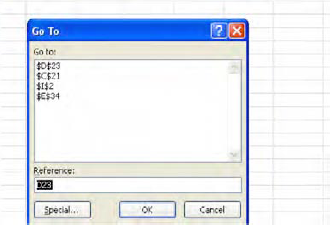
Click any of the addresses recorded and click OK, and you'll be returned to that address (those dollar signs will be explained in a later chapter). (Go To also does a number of other more exotic things, too, such as flagging all the worksheet's cells with formulas in them, if you need to know that sort of thing.)

Here's a table summary of these options we've described (the list is not exhaustive, by the way, but will surely do for now):

And now for something if not completely, then at least slightly, different. To date, we've explored a variety of ways for meandering across the worksheet, all of which bring us to one particular cell at journey's end. But Excel also provides us with the means for occupying more than one cell at the same time. What does that mean?

Well, it means that it's time to dust off another one of those have-to-know concepts. This matter doesn't originate with Excel, of course, but history aside, spreadsheet users very often need to visit, work with, or be able to identify a group of cells at the same time. Why?

The reasons are several. For example, a user may want to change the font that currently appears in a large cluster of cells. Having the ability to bring about that change simultaneously in all those cells is obviously a great deal more efficient than having to revise each cell individually. After all, what if you wanted to change the font for, say, 50 million cells?

In addition, Excel users very often need to perform some sort of mathematical operation on a gaggle of cells at the same time. Indeed, isn't adding rows or columns of numbers—the classic Excel task—exactly what we're talking about here?

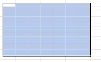
So in order to do this kind of work we need to be able to define ranges on the worksheet. Strictly speaking, a range is any collection of cells that has been selected or identified at the same time. But more conventionally put, a range is a set of adjacent cells that exhibit a rectangular shape—and the concept is far simpler than it sounds.

Figure 2-10, for example, is a range:

Figure 2.10. A typical range

As is Figure 2-11

Figure 2.11. Another range example, this one narrower and shorter

And so is Figure 2-12:

Figure 2.12. One column, eleven rows

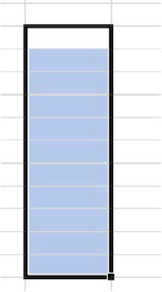
You're doubtless getting the idea. Our cell pointer—and that's what it is—stretches when it selects a range, serving as its perimeter; and with one clear exception, a bluish fill color identifies exactly those cellsthat populate the range (and why the very first cell in a range remains white is a matter to be revealed later).

And so here's the point behind all this: if I want to change the font in a range of cells, I can select those cells I want as illustrated above, and then go ahead and issue a font-change command. And as a result, only the cells in the range will be affected.

And how do you go about selecting cells in a range? It's rather easy—and again, both mouse and keyboard approaches stand at the ready. If you're mouse-inclined, click the first cell of the desired range—which is, typically, the upper-left cell in the block of cells you want to select. Keep the mouse button down, and pull—or drag—across and/or down the cells you want to incorporate into the range. When you're done, release the mouse button, and the blue-blanketed range remains selected.

You can also select an entire column by simply clicking a column header—that is, the alphabetized area in which the columns are named. Doing so highlights that column, as in Figure 2-13:

Figure 2.13. An entire column selected

Yes—all one-million-plus cells in the K column are now selected (hope you weren't expecting a fold-out showing them all). And you can select a row by clicking one of the numbered row headers on the side of the screen. And by clicking the column/row header area and dragging across or down that area, you can select multiple columns or rows.

And if you opt for keyboard cell-selection approaches, first select that upper-left cell, using any navigational means you wish. Then hold down the Shift key, keep it down, and press any of the keyboard arrow keys in the direction of the cells you wish to select. For example, you can first press the Right and then the Down arrows, thus enabling you to describe a range of as many columns and rows as you wish. Just remember to keep the Shift key down throughout the process. When you're done, release the Shift key and observe your range, decked out in blue. (Just keep in mind for the record that you could start your range selection by clicking what is the upper-right cell of the desired range, and dragging left and down and/or up. It's just that most people—at least those who speak and write English—tend to think left to right.)

But I've been holding out on you. There's yet another way to designate a range, and that alternative takes us back once again to the name box, along with an important data entry principle. If, for example I type this:

in the name box and then press Enter, cells D13 through H23 will be selected, turning that tell-tale blue (with the exception of D13, which serves as the "first", upper-left cell in the range and so remains white). Note the expression—D13:H23. It means that all the cells from D13—the upper-left cell in the range—through H23—the lower-right cell in the range—have been designated for the range selection; and this upper-left/lower-right-cell nomenclature for range boundaries is indispensable to Excel formulas. Thus, by way of preview, if you see an expression that looks something like this:

You'll know it means that all the numbers in cells A34 through C57 are to be added (And by the way – this formula: =SUM(A:A) – would add all the cells in the A column).

One more point (for now) about ranges. Consider this possibility, shown in Figure 2-14:

Figure 2.14. Two ranges selected at the same time

So what's going on here? In this case, two ranges seem to have been selected at the same time. How's that done? Truth to be told, rather easily. First, select one range as per the usual techniques. Then, keep the Ctrl key down, and with your mouse, drag across a second set of cells. You can even select three or more sets of cells with this approach—and if you're wondering why you would want to do such a thing, the answer is that you may wish to subject all these cells to the same change—you may want to alter the font size in just these selected cells, for example. Or you may want to delete the contents of a range or two of cells. If you do, select the range(s), and just press the Delete key. (And let's pass on the question about whether the screen shot above depicts two different ranges, or merely one range consisting of two non-adjacent sets of cells. In reality either answer could apply depending on your purposes, but in the great majority of cases you'd be regarding these as two distinct ranges.)

And if you want to try something a bit more exotic, you can also type something like this in the good old name box, followed by pressing Enter:

Note the comma. The above instruction will select cells A3 through D34, as well as E6 through H23.

And if you mess up—that is, if you select the wrong set of cells—the easiest thing to do is simply click anywhere on the worksheet. Doing so "turns off" the blue color scheme for the selected range, and you can start range-selecting again. And in any case, you're going to need to turn off the range sooner or later if you plan on doing work anywhere else on the worksheet.

Now if you really need to change the font for 50 million or so cells—or something even more global—try this. It's easy to overlook, but observe the button wedged between the A column and row 1 headings...Click it and all 17 billion cells turn blue (excepting A1 above. You can also press Ctrl-A to select all the worksheet cells). You've thereby selected the entire worksheet, and you might opt for this mass procedure if, for example, you wanted to change the color of all the text in your worksheet to say, green. Once you're finished, just click anywhere on the sheet, and the blue selection color disappears, as in Figure 2-15:

Figure 2.15. Click here to select all the worksheet cells

A last introductory point about ranges. Like amoeba, ranges can be single-celled, and if you're at a loss to understand why—after all, how in the world is selecting a one-celled range different from simply referring to a single cell?—stay tuned. There are sometimes very good and productive reasons for working this way. (Note: See the appendix on range names for a discussion of this and other range-related tips.)

But now that we've learned how to get where we want to go on the worksheet, let's learn the things we can do once we arrive. There are a few billion cells out there craving our attention, and we want to fill at least some of them with data. Here's how.

Unlike typing in Microsoft Word, data entry in Excel is a two-step, but still elementary, affair. Type the number 48 in Word, for example, and you're done. But enter 48 in a worksheet cell and you need to complete the process by installing the value in the cell. And that second step is carried out either by any navigational move away from the cell (e.g., pressing Enter or Page Down, or clicking a different cell) in which you've just typed, or by entering the value and then clicking the check box alongside the formula bar, as shown in Figure 2-16:

Figure 2.16. Click the check to place the value in its cell.

Here's the simplest-case scenario. Type 48 in cell A3 and then press Enter. You've just done two things:

Remember you need to execute two steps in order to enter data: Type the value, and then finalize the entry with some navigational move (including Ctrl-Enter, which actually leaves you in the cell), or by clicking the check mark.

But if you have second thoughts about entering that value, you need only press the Esc key before you install it in the cell, or click the X you see above alongside the check mark. Do either of these things and the value simply won't make its way in the cell. Note also you'll only see the X and the check mark on screen when you start to type in a cell.

(Note that for our purposes, we'll always tell you to press Enter in order to enter data in their cells simply as a matter of explanatory convenience. But remember that you can use the other options, too, unless I state otherwise.)

It's rather easy, and it should be—so don't wait for the other shoe to drop. There are no hidden complexities here. Still, a number of classic data entry features and issues need to be explained, just the same.

Entering Text: Trespassing Allowed

For one thing, note that when you enter a number it's pushed by default to the cell's right border, or aligned right, as they say in the trade. That's because our number system is Arabic, and proceeds from right to left. Enter text, however—and text are data, too—and the results align left, as per our left-to-right, Roman alphabet.

Now if I type something a bit more extensive—say, the phrase "Microsoft Excel"—in A3, the result looks like Figure 2-17:

Figure 2.17. Run out of space?

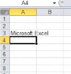
thereby raising an ancient spreadsheet question. You'll note that our phrase appears to overrun cell A3 and invade the neighboring B3, implying in turn that the text occupies two different cells—but that isn't the case. In fact the entire phrase is still positioned in A3, appearances notwithstanding; but apart from the fact that I've done this a few thousand times, how do I know that?

I know it because I can direct my attention to that long strip to the right of the name box, called the formula bar (and again, we'll need to explain that name). Click cell A3 again and check out the formula bar—you'll see Figure 2-18:

Figure 2.18. The Formula Bar: recording the actual contents of a cell

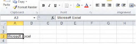
Note the visual relationship in force here. I've clicked on cell A3. The formula bar records what I've typed there, confirming that the phrase in A3 indeed occupies that cell, and only that cell. If you need additional proof, click cell B3 and turn to the formula bar—which now shows...nothing.

Yeah, this is another have-to-know, actually a few of them. First, we've learned that whatever you type in a cell is wholly confined to that cell, no matter what optical illusions are perpetrated on the worksheet. Second, we've learned that the formula bar tells you exactly what's going on in the cell you click, a point that will acquire additional importance as we proceed.

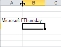
But there's more to this. If I go ahead and actually type something in cell B3—say, "Thursday"—the worksheet reports what you see in Figure 2-19:

Figure 2.19. The case of the disappearing word

Now, Houston, we have a problem—a rather obvious one. We have seen that as long as the adjoining cells to the right remain empty, it's perfectly permissible to enter a lengthy phrase (at least one comprising text—more on this soon) in a cell, even if its contents encroach on the nearby cells. But type anything—even one character—in one of the adjoining, empty-till-now cells, and the cell reclaims its own turf, barring any excess text from other cells to its left. As a result, you'll have two obvious questions: Has the clipped text in cell A3 been somehow deleted, and, whatever the answer to that question, what do we do next?

The answer to the first question is: No. Click back on cell A3 and scan the formula bar. You'll see that the phrase "Microsoft Excel" is intact. None of it has been deleted, but rather some of it—that segment which had spilled into B3—has been obscured by the text entered in that latter cell. And that's what happens to text if it exceeds its column boundary: it continues untouched across empty, adjoining cells—until one of those cells is empty no longer. It's then visually restricted to its own column.

And as for question two: If we delete the entry in cell B3, then all the text in A3 reappears on screen. But if we want to keep "Thursday" in its place, we need to widen the column in which "Microsoft Excel" resides—in this case—the column A. Doing so should make room for all the text in both cells.

There is, as is usual with the Office programs, more than one way to do this. The two easiest and fastest are carried out as follows:

With your mouse, move up to the right boundary of the column you wish to widen (and not row 1). What started out as Excel's familiar thick white cross—the one you see when you move about the worksheet proper—should now appear as the slender, black, double-arrowed object seen in Figure 2-20:

Figure 2.20. The A column, selected for widening

You must bring about that double-arrowed pointer in order to widen the column; but it should appear automatically as soon as your mouse arrives atop the right boundary. Then click the boundary, and drag to the right (don't release the left mouse button). As you do so, the column should expand, revealing ever more of the text. And as you drag, a caption accompanies the action, tallying the current column width both in units of text characters and pixels (this bit of information is usually of little more than academic importance most of the time; just bear in mind that the default width of an Excel column is set at 8.43 characters, for historical reasons). When you've achieved the desired width—presumably after all the hidden text has been brought to light—you can release the mouse. Nothing stops you from widening—or narrowing—the column again, by dragging it again to the right or even to the left. If you've accidentally clicked on the left boundary of the column you want—which is, after all, the right boundary of the column to its left—then that column will be widened instead.

Bring your mouse to that same right column boundary, make sure the double-arrowed cross is in view, and this time double-click. The column will automatically resize itself to reveal all the data in the column. Known as Autofit, this rather efficient device is a time-honored means for solving the hidden-text problem. Note that Autofit modulates the column to make sure to reveal what is currently its widest entry, fitting itself snuggly to that entry's width; and so if you delete that item from the column and perform another Autofit, the column may narrow, as it hugs what is now the widest entry.

Now for an important variation on the Autofit theme, here's a scenario you might very well have to confront. Suppose you've entered the months of the year, and your data look like Figure 2-21:

Figure 2.21. Columns in need of widening—or narrowing

The problem is clear: some of the longer month names have barged into the cells to their right, and these happen to be occupied by months of their own. Thus the same column-width issue emerges; but what's new here is that we can conduct an Autofit on several columns at the same time.

To make this happen, click the first of the column headings—A—hold the mouse button down, and drag across the remaining headings (again, don't drag across row 1 on the worksheet; you need to select the headings). Your worksheet would look something like this, as shown in Figure 2-22:

Figure 2.22. Columns selected and prepared for autofitting

That blanket of blue cells teaches us incidentally that when you click a column heading, all the cells in that column are selected; but what interests us here is the column width question; so now double-click any one of the boundaries separating any of the selected columns, e.g., the one separating B and C, or J and K (again, you'll need to see that double-arrow cross). All the columns should now be resized, with each new width reflecting the respective widths of the months. See Figure 2-23:

Figure 2.23. Autofit: one size doesn't fit all

It's a nifty way of Autofitting lots of columns in one go; but now you may have to contend with another possible problem. Thanks to Autofit we can now see all the text, but since each of the months exhibits a different width, so then do the columns housing them—and presentationally speaking, that may not look very nice. You may want uniformly widened columns instead, but you can't get there from here using Autofit. What to do?

The answer is to select all the column headings as described above, but this time, instead of double-clicking any boundary, we click the right column boundary of the longest month—in this case "September," given the font being used—and drag a bit to the right. Then release the mouse. This technique—really a variation on the first column-widening approach we cited earlier—equalizes the width of all the selected columns; and because we dragged on the widest month's column, naturally all the other months should be visible as well. And if you drag and release the mouse too soon and fail to reveal the word "September" in its entirety, note that all the columns remain selected, so you can resume dragging until the word is completely exposed.

You'll also want to know about another data entry option, one you'll have difficulty ignoring in any case. If you enter text down consecutive cells in a column and have occasion to enter the same datum (that's the singular, believe it or not) twice in different cells, Excel will automatically enter it for you the second (and every subsequent) time in the cell in which you're typing, as soon as it recognizes it. That is, if you enter "John" in cell D2 and "Bill" in D3, and then begin to enter "John" in D4, Excel will complete the name "John" as soon as you type the letter J (this will happen even if you type a lower-case j. See Figure 2-24:

Figure 2.24. AutoComplete in action; note the formula bar

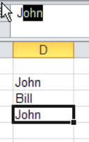
That is, Excel will try to AutoComplete the name. If you approve of the suggestion, simply press Enter. But if you really want to type "Jerry" in D4, just keep on typing. Note that if you've already entered "Mary" and "May" in different cells, you'll need to type the third letter in either of these names, as Excel won't otherwise know which name you wanted to AutoComplete. But again, if you want "Martin" instead, keep on typing.

But what is entirely possible to ignore is another, related feature. Once you've typed even one name with the intention of continuing to type down a column, you can right-click the next cell, and take note of this option in Figure 2-25:

Figure 2.25. Your on-the-fly drop-down list in the making...

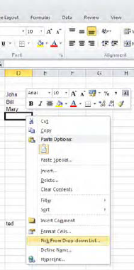
If I click here, the menu shown in Figure 2-26 appears:

Figure 2.26. ...and here it is

It's a mini-drop-down, grabbing its data from the current list of names you've typed in the list to date—and the list incorporates any new names as you type them. Just click one. Cool, and little known.

Now let's return to the business of data entry proper, because to date we've omitted a rather essential form of data from the discussion—numbers. The mechanics of numerical data entry are identical to those governing text: Just type the number, and then execute one of those moves away from the cell. Don't worry about typing commas and dollar signs for now; just type the number. Note by way of introduction that if you type:

for example, the number will appear just as you've typed it. But if you enter:

you'll see 56 only, because by default Excel sheds those meaningless zeros—until you format it differently (but if you reformat the number, remember it really remains nothing but 56. A glance at the formula bar will provide that confirmation). Note in addition that a number less than 1, say .78, will appear by default as:

that leading zero can be removed by a customized format, about which we'll have more to say later.

And you'll soon discover a couple of other issues that apply to numbers only.

For one thing, and unlike with text entry, Excel will never permit a number to advance into an adjoining column, even if that column is vacant. The reasons are fairly clear. Because our numbers move right-to-left, allowing a number to break into the column to its right would hopelessly misalign a set of numbers streaming down one column. If, for example, a 12-digit number in A4 were to take over some of the space in cell B4 because of its extreme width, and a merely 3-digit number were to populate A5 just beneath it, the "ones" column in the two numbers would be out of whack. The "ones" in A4 would be shunted into B4, even as the "ones" in A5 would remain in A5.

Moreover, if that long number in A4 were allowed to ooze into B4—as happens with text—and a number were then entered directly into B4, you'd find it difficult to know A4's true value—because some of its columns would be clipped from view, again as with text. The whole thing is just too messy, and as a result, numbers do not enter adjacent columns.

So what does happen, then? That depends. If you type a 12-digit number in a column with the start-off, default column width in effect, say

You'll see this instead:

If you haven't seen a number like that lately, it means you graduated high school a long time ago. The long number is rewritten in scientific notation, a kind of shorthand that hems the number into its existing column width, thus keeping in it view, though the number as you typed it is displayed that way in the formula bar. But you can reformat the number into the original value you typed—as you almost surely will—and when you do reformat it, Excel then accompanies the process with an Autofit on its own to display the number in its entirety, as you originally entered it (and we'll see how to apply this and various other number formats in Chapter 4).

If, on the other hand, you type a long number and then for whatever reason narrow its column substantially, you'll see this:

—another classic spreadsheet indicator. Seeing those pound (or hash, or number sign, if you live in the UK and other distant locales) signs in a cell means the cell contains a number that is too long for its current width—and you see pound signs there instead of the scientific notation when you actively narrow the cell. The solution: do an Autofit.

Now here's another indispensible form of data entry you need to know about, though it isn't generally characterized in those terms—copying and moving data.

After all, when you copy data you're reproducing, or entering, more of it, and Excel's copying options are several, and don't always resemble the sorts of things you'd do in Word. Let's explore some of the permutations.

We'll start of course with the basics. Say I want to copy values or text—and let's begin with one cell's worth of data:

Note as well, however, that even though you've done your job, the marching ants continue to troop around the cell border—at least if you click Copy or press Ctrl-V (but not if you press Enter). That's not a cue for an exterminator, but rather an indicator to the effect that you can paste the cell again to other cells, with repeated pastes. When you want to turn the process off, just click the Esc key, and the ants recede. Note that if you paste with Enter, the ants immediately disappear. How about copying a range of cells? This time:

Note that when you paste a copied range Excel preserves the orientation of the cells in question. That is, if you copy a column of cells, Paste will always paste these in columnar fashion, and a copied row will always paste as a row (yes, you can paste a column into a row orientation and vice versa if you want to, but that's for a bit later).

And what of moving data? That's what we really mean by cutting and pasting, and the process is rather easy:

Note that with Cut and Paste the marching ants retreat after one Paste. That's because, well, what's the alternative? The data have been cut and moved elsewhere; granting users another Paste means they'd want to move the data again immediately—a not terribly likely prospect.

There's an alternative way to move (and copy) data in cells, though this one requires a bit of delicacy. Select the range you want to move and rest your mouse anywhere along the range's perimeter, until you see a pair of double-sided arrows. Then click and drag the range to its new destination, and release the mouse. If you do the same thing while holding the Ctrl key down, you can copy the range. These techniques are fairly easy to mess up, though; releasing the mouse too soon will let the data down in the wrong place.

Now there's still another way to copy cell contents, this one also mouse-powered, and it works like this: We'll start with a number in one cell. Click the cell and slide your mouse atop the lower-right corner of the cell pointer border, where you'll notice a small square lodged in the corner, like a dimple. When you roll the mouse over that little shape, your indicator should remake itself into a slender black cross, as shown in Figure 2-28, not to be confused with the black double-arrow variety you generate when you widen columns:

Figure 2.28. The fill handle

When that cross appears, click and hold the mouse button down. Drag as far as you wish, either across a row or down a column, depending on the direction in which you want to copy. Release the mouse when you've dragged the desired distance; you'll see the original number has been copied down or across the range you've dragged. You'll also doubtless take note of the caption that escorts you down/across the range as you drag; it tells you what value will appear in each cell in the copied-to, destination range as you drag. But because, in this case, you're simply copying the same number to each cell again and again, you may think that the caption tells you something you already know—and you're right—this time.

We've just demonstrated an application of what's called Auto-fill, a device that can serve you most productively once you learn its capabilities. And that square dimple we dragged is called the fill handle, and you'll want to handle it with care.

And you'll notice something else. When you've completed dragging, Excel caps the process by appending to the lower-right corner of the new, copied range what's called an Auto Fill Options button. Click it and four selections place themselves at your service. We'll discuss the first two here, because the latter two carry out formatting options, which aren't our concern here. Take a look at Figure 2-29:

Figure 2.29. Auto-fill options

The default selection, Copy Cells, really characterizes what we've just done. But assuming we've copied the number 3 as per the screen shot, from the D17 source cell down through D30, look then what happens when we click selection number two, Fill Series, as shown in Figure 2-30:

Figure 2.30. A Fill Series

I'll bet that one got you to look up and stop texting. What Excel has done here is add an increment of one to each of the cells in the range to which we copied the original value, 3. That's a rather cool capability (and it hasn't debuted in Excel 2010, either—this option goes way back), and we're just getting started with it.

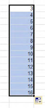
Now try this: type the numbers 3 and 5 in cells G3 and G4. Then select both cells and release the mouse. Next, Click and drag the fill handle down the G column to G10. You should see this (Figure 2-31):

Figure 2.31. Getting a handle on the process: A fill series displaying an interval of 2

Here, Excel works with two starting cells, containing the numbers 3 and 5; these alert the worksheet about the interval that will pump up all the numbers in the range. As per the Auto Options button command, we've generated what's called a Fill Series, and we could have dragged the fill handle down thousands of cells had we wished, with each successive cell displaying a value 2 higher than the preceding one. And if you start with 5 and 3 instead of 3 and 5 and drag the handle, the numbers will descend in decrements of two, e.g., 5, 3, 1, −1, −3, etc. Nor is Excel intimated by exotic intervals: if you enter starting numbers of say 1.36 and 2.43, Auto-fill is perfectly happy to roll out 3.5, 4.57, 5.64, and the like. Just keep this caution in mind: in order to carry out an Auto-fill properly and avoid a common mistake, don't, for example, type 3 and 5 and return to the 3 and begin dragging. Rather, you must select 3 and 5, release the mouse, and then return to that selection and drag the fill handle. That is, you must see this, shown in Figure 2-32, before you start the fill process:

Figure 2.32. Learning to let go: release the mouse before you drag here.

Now get this. If I type any day of the week in any cell and drag on the fill handle (it's always there; you just may not have paid it any mind till now), this is what happens (Figure 2-33):

Figure 2.33. Cells-by dates

Rather economical, isn't it? I started here with Tuesday and dragged horizontally, and could have dragged as far as I wanted. (Yes, the column widths may need tweaking, but you know how to do that now.)

And if I type any month and drag on the handle, I bet you know what's going to happen (Figure 2-34):

Figure 2.34. 30-day guarantee...filling the months

Moreover, I can do the same with three-letter day or month abbreviations. Type Wed, drag the fill handle, and you get Thu, Fri, Sat, etc. Type Jul and Aug, Sept, Oct, etc. emerge.

These four Auto-fill routines—day, month, and respective three-letter abbreviations—are built into Excel. But you can construct your own lists, too, such that when you type any one of its names and drag the fill handle, all the other names streak onto the screen. How?

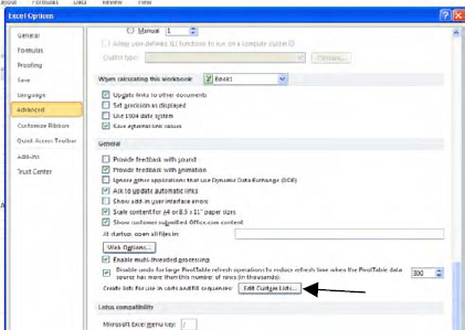
Like this. Click the File tab, and then Options (in the left column), and click again on Advanced. Scroll down the window—pretty far down, until you approach the end and see the Edit Custom Lists button (Figure 2-35):

Figure 2.35. Try this at home...where to start making your custom list

Click and you'll see (Figure 2-36):

Figure 2.36. Note the existing lists, supplied by Excel.

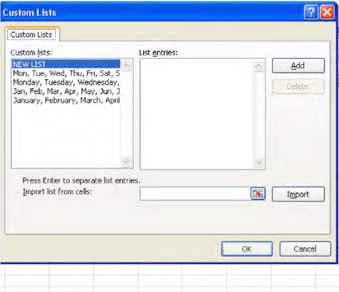
Click in the List entries area and type each name you want to appear in your list, and in the desired sequence, following each entry with Enter, as shown in Figure 2-37:

Figure 2.37. Where the list takes shape

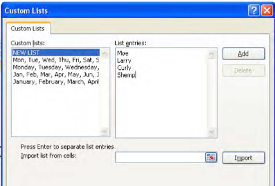
When you're done, click Add, and your list is swung into the Custom Lists column, where it now shares a zip code with Excel's built-in, default lists.

Then just type any one of your custom names in a cell, drag the fill handle, and your list plays down or across the range.

Just bear in mind that we haven't exhausted all the possibilities for copying and moving data. That's because a different kind of cell content—a cell reference—can also be copied or cut, with some new implications. That one is coming soon.

Now on to some concluding observations about basic data entry. Note that this expression:

is considered text. Indeed, for starters, any data entry containing a non-numerical element, such as:

or say, a social security number:

is to be treated as text, as opposed to a number. You can't add a social security number; and Excel won't treat the number above as a case of subtraction, either. You'll soon see why.

Now there's one other basic data entry principle you'll want to know that will at last shed some light on that pristine white cell you'll always see topping a range selection. Again, if I go ahead and drag my mouse across a range of cells:

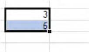
There's that ever-present white cell. And what purpose does that cell serve? It marks the cell that will receive the next bit of data you type. Select a range, begin to type, and then press Enter. The entry ends up in the white cell.

And if you need any corroboration, select any range, observe the address of the white cell, and glance in turn at the name box. You'll see that very address recorded in the box.

And the white-cell/range selection does something else. If you select any range and begin to type, the first entry stakes the white cell—and if you press Enter, the cell pointer plunges down one row, of course—but the blue range color remains in force. Try this: select cells D12 through D21, type the number 51, and press Enter. This is what you'll see (Figure 2-38):

Figure 2.38. Within range—data entry inside the selection

Type a number in the current cell—D13—and press Enter, and the number is once again registered in its cell—and the pointer again descends one row, to D14. And so forth.

But of course you'll have a question about all this: Entering data in a cell and pressing Enter always does exactly what I've described above—even if you don't select a range. So what are we gaining here?

Here's the answer: Select this range instead: D12:E21. Start typing and press Enter. The data locks into D12 and proceeds to D13, etc. But when you reach cell D21—the last cell in the D column—and press Enter, this time the cell pointer won't drop down to D22—it'll pop up to E12 instead, which is after all the next cell in the selected range (Figure 2-39):

Figure 2.39. Knowing its place: the white cell remains within the range

And when you reach cell E21—the last cell in the range—and enter data there and press Enter, you'll be taken back to D12.

This, then, is the data-entry advantage of selecting a range, if you need to: the range selection confines your data entry to precisely that area of the spreadsheet and nowhere else. But note, however, that if you follow up each data entry in the range by carrying out some of the other navigational moves instead of Enter, such as pressing the various keyboard arrows, or clicking your mouse, the blue range selection will turn off and the method we've just described will likewise be voided—unless you select the range again, of course. If you do want to conduct your data entry within a specified range, these keystrokes work:

That concludes our discussion of the basics of data entry—but not to worry; we need to return to the subject. There's all that formatting to do, after all!

But in any case, once you nail down the basics we still need to remind ourselves that no one's perfect, and in the course of imparting their data to worksheets users make mistakes, change their minds, and have to enter new numbers as events warrant. So once the data is squirreled into their respective cells, we still need to ask: how do you edit all this?

As you'd expect, there's more than one way to modify the contents of cells, all of which are pretty easy to master. The most straightforward approach is to simply overwrite any existing cell contents; that is, just click or key your way into the cell you want to overwrite, and type something new. That's all.

Another rather obvious and decisive editing tack of course is to simply delete the contents of the cell(s) in question, if that's what's called for. Just select the cell in question—or a range of cells—and click Delete on your keyboard.

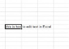
But these appealingly lucid approaches aren't always the most efficient. For example—click any cell and type:

You'll note that the t in this isn't capitalized, but you want it to appear in upper case. Sure, you could retype the whole phrase, but if you're as lazy as I am you'll be searching for a less demanding workaround. Remember that any given Excel cell can hold up to 32,767 characters, and while you're not likely to ever exhaust that capacity, some Excel formulas can be rather dense and ornate, and rewriting them from scratch is an invitation to error. So we need a Plan B to edit this kind of data—and here are three very standard, textbook techniques:

First, click the cell you want to edit and press the F2 key, an ancient command that dates back to the last century (it's been carbon dated). You'll see (Figure 2-40):

Figure 2.40. Inside the cell

Look closely on your screen and you'll see the cursor—that's what it's called—flickering to the immediate right of the last letter of the phrase. You're now "in" the cell, and once you've gained this kind of entree you can carry out word processing-like actions in order to edit whatever you want. Thus here you can press the Home key that, as it does in Word, will take to you the beginning of a line of text. Once there, simply press the Delete key, remove the lowercase t, and replace it with T. Press Enter and you're done. You can edit any character in the cell by pressing the Left or Right arrow keys until you reach the character you want, and then pressing either Backspace or Delete, depending on which side of the character you've positioned yourself. Once in the cell you can also double-click any word, thus selecting it (as you do in Word); you can then either press Delete, thereby eliminating it from the cell, or type something else over it—again, just as you would in Word.

(Note: By clicking off the File

Textbook method #2 reacquaints us with the formula bar, that band of space stretching to the right of the name box, as shown in Figure 2-41:

Figure 2.41. The formula bar revisited

To edit our text via this method, just click the cell containing our text. As usual, you'll see it displayed in the formula bar, as shown in Figure 2-42:

Figure 2.42. What you type is what you get in the formula bar

Then click inside the formula bar, right alongside the lower-case t. Note that when your mouse enters the formula bar area, it acquires a Word-like I-bar appearance, exactly what you see in Word when you move your mouse around text in a document.

And when you click in the bar, the cursor reappears (along with that check mark and X), as you can see in Figure 2-43:

Figure 2.43. Editing a cell inside the formula bar

Then just make any changes as per standard word-processing steps; when you're done, press Enter or click the checkmark. And if in the course of your editing labors you click alongside the wrong character in the formula bar, just click again wherever you want and start to edit.

This last technique is also easy, but requires a measure of care. Let's return to that recalcitrant lower-case t. We can place our mouse over that letter—back in the cell this time, and not the formula bar—and simply double-click. The standard Excel white cross remakes itself into the cursor, at which point you can begin to edit. The caution is this: you can't directly double-click any letter that by appearances has run into adjoining columns. Thus you can't double-click the E in Excel (Figure 2-44):

Figure 2.44. Double-click to edit? That depends.

even though, as previously noted, all the text is lodged in but one cell. Thus, in order to edit the E this way, you need to double-click anywhere within the span of the source cell—in this case somewhere between the words "this is how" and then press your arrow keys or click upon the E and edit. Quirky, but that's how it works. And remember, as per our discussion earlier, you can cancel an edit by pressing the Esc key or clicking the X.

And now that we've found a place for our data, what do we do with all of it? It's time to learn some of the ways you can crunch all those numbers that beckon in your newly entered cells. So just turn the page.