
Now that we've gotten this far, we need to remind ourselves of the obvious: Excel is all about doing something with the data once it's been nestled into its cells—analyzing it, presenting it, and synergizing something new from all those static numbers and text entries; and that reminder takes us to a new domain of have-to-knows—the world of formulas and functions. It's here, once you learn the fundamentals, that you begin to sense the nearly infinite potential of the application—starting of course with the how-tos for adding those rows and columns.
The very first thing you need to know about formulas is that by that term I'm referring to any expression you can write in a cell which conjures something new from the existing data—and it doesn't have to work with numbers, either. Learning which, or how many, students in a lecture class have a last name starting with the letter L or how many major league baseball players were born in Nevada may not be what's keeping you up at night, but if you need to know these things and the basic data are there, there's a formula-based way to find out.
The second indispensible thing to know about formulas is that they always begin with the equal sign. This, then, is a formula:
=3+5
And this isn't:
3+5
That latter expression is pure text, and won't "do" anything more than appear in the cell in which you inscribed it. The voice of experience is speaking: if you write a formula, no matter how ingenious and complex, and you leave out the equal sign, what you get is text.
And since I seem to have written a formula just a few lines ago, let's take a second look at it while it's on hand. Entering =3+5 in a cell will indeed yield the answer you've been looking for: 8, but we need to learn a bit more about the relationship between that answer and the formula that gave rise to it.
Go to any cell, say B6, and type =3+5, followed as usual by Enter or any other navigational optionl such as the checkmark. First, of course, the number 8 stations itself in the cell. Then click back on B6, and take a look at the Formula Bar, shown in Figure 3-1:

Now we know why the Formula Bar is so named. It opens a window on what is really going on in the cell beneath the surface, and in this case of course what you see in the bar doesn't correspond to what you see in the cell. If you print the spreadsheet you'll see the number 8 (by default, anyway), and that's nearly always want you want to see. But you also may need to know that the number was brought about by a formula, and not a simple act of data entry. To glean that bit of information, click on the cell and view the Formula Bar.
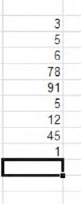
Now, nothing at all prevents you from writing a more protracted formula, such as
=3+5+6+78+91+5+12+45+1
Press Enter and you'll get your answer. Remember, after all—you have 32,767 characters per cell to work with. But for a variety of reasons, spreadsheet users don't like to enter numbers directly into a formula; it's inefficient and a pain to edit, and if you content yourself with this approach you're treating Excel as little more than a PC-based calculator. The far superior way of proceeding is to enter the data you're going to work with in cells, and to work with cell references.
What's a cell reference? It's an expression that, as its name suggests, refers to, or returns, the contents of another cell. Thus if you type the number 45 in cell C6 and proceed to type =C6 in cell C7, that latter cell will display 45 onscreen. If I type Excel in C6, cell C7 will now naturally display Excel. What it won't display onscreen is =C6, even though that's what you've actually typed in the cell.
Now back to our addition example. If I type the same numbers I added above in separate cells, as in Figure 3-2:
and then subject these to a formula instead, we'll achieve the same result—246—but we'll also realize some very important spreadsheet advantages (note that the numbers don't have to be lined up in one column or row in order to be able to add them; they can be strewn anywhere on the worksheet, but we're starting simple).
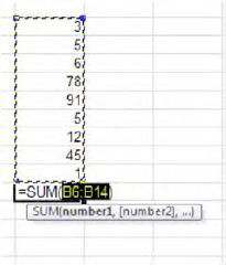
So let's try to add those numbers. Say you type the numbers above in cells B6 through B14. Then do the following:
Click in cell B15 and type the equal sign =
Click on cell B6 and type +. You should see the result shown in Figure 3-3
Click on each of the remaining cells to be added, followed in each case by +.
When you're finished, tap Enter. Your formula:
=B6+B7+B8+B9+B10+B11+B12+B13+B14

Your answer should once again come to 246—but once you achieve that result we need to review the process more closely, because you're asking the obvious rhetorical question: That's a lot of clicking, isn't it? And what if we wanted to add 90,000 numbers instead of 9? Stay tuned...but back to the formula itself.
First, and as stressed earlier, the formula must begin with =. We then clicked on each cell to be added, following each click with +, simply because we're adding the numbers. Had we wanted to subtract some or all of these we would have typed a minus sign instead.
Once we're satisfied we've clicked on the right numbers, we press Enter—or Shift-Enter, Tab, or Shift-Tab, or Ctrl-Enter (or click the checkmark, which in this case actually advances the cell pointer down). And that's how it works. Type =, click each of the cells you want to include in the calculation, followed in each case by a mathematical operator such as + or − (more on this soon), and wind it all up by tapping Enter, or one of the other possibilities cited above. And remember that you can click on cells dispersed anywhere across the worksheet.
And if we've realized our result and then discover we'd made an error in data entry, say, the number in cell B7 is really 15, not 5—all we need do is type the corrected number in that cell, and our formula in cell B15 automatically recalculates to read 256. That's because formulas don't work with particular values as such—rather, they work with whatever values have been entered in the cells to which they refer. And this capacity of spreadsheets – —their ability to recalculate a change in data entry without having to redesign the formula which does the calculation – —may stand as their single greatest contribution to Western Civilization.
Now time for a couple of quick but necessary digressions. First, Table 3-1 shows a list of the basic mathematical operators you can apply to formulas:
Digression number 2. There's another tricky set of rules you will need to understand—or review, as the case may be—because you probably had to put up with some of these in school: the order of operation. For example, what's the answer to this formula?
=4*5+7
It could be 27—that is, 4×5 plus 7—or 48—4×12. Which is it? In this particular case you can resolve the problem by surrounding the relevant numbers with parentheses, e.g.,
=(4*5)+7
Or
You get the idea. Excel resolves this kind of ambiguity with a set of orders of operation—a kind of priority listing which declares which operation takes precedence—that is, is calculated first—in a formula. (In the cases above, the values flanked by parentheses are treated as a unit.) The order reads like this:
Let's illustrate this hierarchy with a few cases. This formula:
=4+5/2
results in an answer of 6.5. It divides 5 by 2 and then adds 4—because priority goes to division over addition.
This formula:
=4*5/2
results in 10, because the multiplication—4 times 5—is carried out first. That result—20—is then divided by 2.
This formula, however:
=4*(5/2)
also yields 10, but this time because the parenthetical expression—(5/2) that is, 2.5—has priority over any other operation.
Now let's get back to our regularly scheduled program—this matter of adding numbers via a formula. While the method we recounted above surely works, it conceals a problem. What if you need to add 20,000, or even 200, numbers? You won't want to click on each and every one of those cells as per our initial method—and, given Excel's cell character limit, you may not be able to do it anyway. So what's the alternative?
Good question. The answer takes us to the first and most important of Excel's built-in operations, or functions, called SUM. How does SUM work? For introductory purposes, we'll demonstrate the standard way to implement SUM in a worksheet—with the AutoSum command, which is actually stored in two different tabs (remember that term?) in slightly different guises—Home and Formulas, shown in Figures 3-4 and 3-5:


And once you appreciate how AutoSum works—and it's rather simple—you'll go a long way toward firming your grasp of the whole function genre.
So let's try the following: click on the Home tab, if you're not already there. Delete your answer in cell B15, stay in that cell, and click AutoSum. You should see Figure 3-6
Then press Enter, and presto—your answer should materialize.
You see what's happened. AutoSum installed a function—SUM—into the cell in which you clicked, a cell that happens to be positioned directly below the range of numbers we wanted to add; and that's a range SUM automatically identified. That's why it's called AutoSum.
But before we return to the workings of SUM in particular, note some very basic principles of Excel functions. First, apart form the equals sign (=), an open parenthesis always follows the name of the function—here, SUM. Then some additional information—which could be a range and/or some other entries, as you'll see—follows, after which the expression is concluded with a close parenthesis. To summarize the basic syntax for any function:
=NAME(various data in here)
Remember that the equals sign always appears at the outset of any formula, e.g, =67+SUM(B6:B15000). (Here we're describing the basic syntax of a function considered alone.) What kind of data gets interposed between the parentheses depends on the function, as you'll see; here, in our current case, SUM identifies the range to be added.
Now back to AutoSum. We see that AutoSum indeed correctly identified the range we wanted to add—and had that range, for example, been B6:B15000 instead, we could have clicked on cell B15001, and proceeded to click AutoSum. We'd then see this in B15001:
=SUM(B6:B15000)
We'd go on to press Enter, and the numbers in all those cells would be added.
Thus we're beginning to infer what exactly it is that AutoSum does. It's programmed to automatically identify a range of consecutive numbers to be added in the column or row in which you've clicked. And you needn't click in the cell immediately below the column or immediately to the right of the row containing the numbers—just somewhere in that column or row. Thus AutoSum will work in the example shown in Figure 3-7, too:
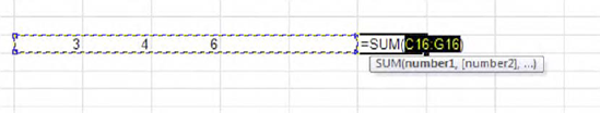
Starting to get the point? Here we're adding a row of numbers, even as we've spaced the AutoSum cell two columns away from the last number—and Excel doesn't mind. And look at the range SUM identified—it's included the two empty cells to the left of AutoSum, as the formula itself appears in H16.
In sum (pun intended) and by default, AutoSum will begin to total all consecutive numbers in the column or row in which it's been positioned. But what if you see something like Figure 3-8 in cells C18 through C24?
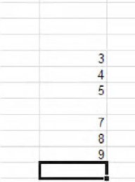
If you click on cell C25 and turn to AutoSum, the resulting formula will read (Figure 3-9):
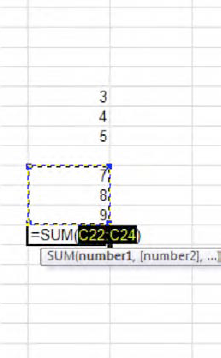
What's wrong with this picture? You want to add C18 through C24—and what you get is C22 through C24.
But you may now understand why. AutoSum designates ranges consisting only of consecutive number-bearing cells; and in the case before us there's an empty cell—C21—which breaks the continuity. And so AutoSum frames a range that extends only as far as the consecutive string of number-bearing cells closest to it. That's why we see C22:C24.
But we want to add cells C18 through C24. When I've presented students with this problem, many have replied that a zero could be entered in the vacant cell—a worthy suggestion, because a zero naturally won't alter the sum we want to compute, and because it contributes a longer, gap-free range to the formula—C18 through C24. But I strongly advise against this tack—even though the answer it proposes is correct. Because if you go ahead and also compute the average of the numbers in C18 through C24, the zero will heavily skew the result—because zero is a number, and a blank cell isn't (as we'll soon see).
The by-the-book way to solve the puzzle, then, is to click in cell C25, click AutoSum, and then drag cells C18 through C24—in effect, overriding AutoSum's original (C22:C24) recommendation, as seen in Figure 3-10:

Figure 3.10. Drawing a blank: or rather, drawing your range over a blank cell separating two sets of numbers
As an alternative, nothing prevents you from typing the correct expression in the Formula Bar; but dragging the desired cells may be visually easier to track. Then press Enter, and all the desired cells are added. (Don't, by the way, accidentally over-drag into cell C25—because that cell contains the formula itself, and you can't incorporate it into its own result. That kind of miscue is called a circular reference (and Excel will deliver an onscreen error message to you to that effect), whereby the cell adds itself, as it were—and that causes way too many problems).
Thus we see that the initial range drawn up by AutoSum is merely a friendly suggestion, yours to accept or reject, and one you can replace with a different range if events warrant.
And along these lines, suppose you wanted to add the numbers in Figure 3-11, deposited in cells C14:C16 and E14:E16 respectively:
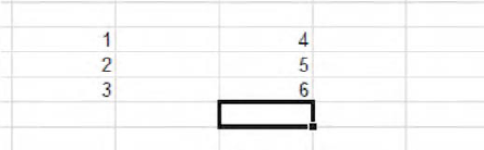
First, we need to decide the cell in which we want our answer to appear. In the interests of simplicity, let's choose cell C17. We click AutoSum, and are presented with the range selection seen in Figure 3-12, of course:

Now we have a decision to make. Because we want to add both ranges, we could next drag across all the cells in question, as in Figure 3-13:
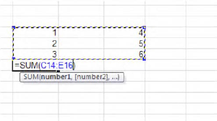
Figure 3.13. Kind of a drag: spanning two ranges to be added in one SUM. Note, however, that the function treats these values as one range for formula purposes: C14:E16
And that's what you probably would do, after which you'd press Enter and return your answer. But suppose there were an additional set of numbers in those in-between cells D14:D16—and you don't want these incorporated in your answer. If we proceed with the range selection we've just named—C14:E16—the numbers in D14:D16 will be brought along, because they too inhabit the selected range. So how do we exclude these unwanted cells?
We can do the following:
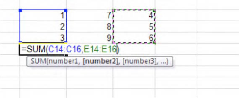
Click AutoSum, yielding the initial C14:C16 range selection. Then type a comma (don't add a space) and drag range E14:E16 (you can also hold down the Ctrl key after selecting the first range, and then select E14:E16 (Figure 3-14):
Then press Enter.
You get the picture. The comma splices our cell selections into two distinct ranges, thus leapfrogging the D14:D16 cells.
We've now learned a deeper truth about SUM, one that can be projected to all functions: you can identify any cell or range(s) you want in any formula, and place your formulas in any cell in the worksheet (so long as the formula isn't dropped into the very range you're referencing in the formula). Remember that AutoSum was devised in order to execute a simplest-case scenario, the spreadsheet equivalent of a hanging curveball—that classic, add-one-row-or-one-column chore, where the row or column to be added consists of a range, all of whose cells are filled with numbers. But your formula requirements may be more nuanced, and the reality is that you can recruit cells and ranges from all across the worksheet—and even beyond it, as remains to be seen.
Note as well that nothing whatever stops you from typing SUM if you're so moved, or any other function in Excel, for that matter. As long as you know the syntax, you're free to tickle the keys as wish; and as we'll see, Excel offers you a number of ways to see to it that whatever you're writing turns out correct.
And here are some AutoSum shortcuts: The keyboard equivalent for calling up the command is Alt+=. And if you're working conventionally, and you know you want to add a standard range of consecutive numbers in a column: just click in an empty cell at the foot of the column and double-click the AutoSum button (as it appears in either the Home or Formulas groups). Double-clicking cuts immediately to the answer, without requiring you to make any additional range decisions.
And one more observation about AutoSum: if you rest your mouse over either of its buttons, the resulting caption tells you that AutoSum helps you "Display the sum of the selected cells directly after the selected cells". But we know that isn't quite true; as we saw earlier you can leave some space between the numbers (as long as these are consecutive) and the formula itself in that column or row and still get AutoSum to work for you, though those empty cells will also be referenced in the formula.
Now, you'll note that both AutoSum buttons on either tab are accompanied by one of those drop-down arrows we alerted you to a good many pages ago (Figure 3-15):
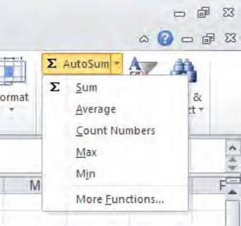
Click the arrow and you'll see a small list of additional functions, and pretty important ones, ones I've used a million times:
Sum
Average
Count Numbers
Max
Min
How do these work and what do they do? To answer those questions in order—these functions behave virtually identically to SUM, in the sense that they're written in the same manner, with the same kinds of range references and issues as described above. Moreover, each of these has an "Auto" character—meaning that if you click beneath a column or to the right of a row of numbers, you can click on their names and install them in the desired cell—just as with AutoSum.
Now let's explain what these functions actually do.
AVERAGE is a spreadsheet staple that performs as advertised—it computes the average of a range, or a set of selected cells. Again, its structure is a virtual clone of SUM, so for example:
=AVERAGE(D23:D42)
returns the average of that range. As implied earlier in our discussion of SUM, AVERAGE ignores any blank cell in a range, refusing to treat it as the mathematical equivalent of zero. Thus AVERAGE yields a result of 8 for the range below, and not the 6.4 you'd compile if the blank cell were assigned an ad hoc value of zero.
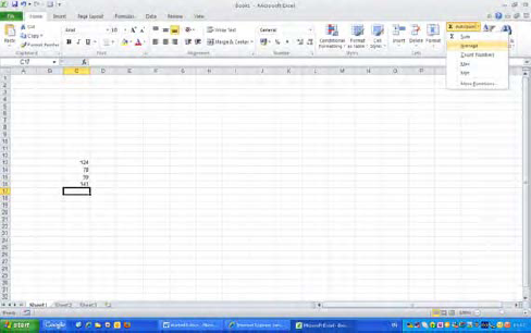
And once again, if your data are arrayed conventionally in one column or row, you can click on Average in the AutoSum drop down menu, press Enter, and AVERAGE will be posted in the cell you've selected (Figure 3-16):
You can incorporate multiple ranges in AVERAGE as well. (Your decimal point questions will be taken up in the next chapter).
And what about the third entry in the AutoSum drop-down menu, Count Numbers? Here Excel's menu description doesn't quite match the actual name of the function it generates —COUNT—and for a reason, which we'll explain right after we let you know what COUNT actually does. (Figure 3-17):

COUNT simply counts all the cells in a range (or ranges) which contain numbers—nothing more mathematical then that. Thus in the above screen shot, if I click cell C17 and select COUNT—and the method for doing this is identical to AVERAGE and SUM—I'll drum up a result of 4. But substitute a text entry for any the cells in Figure 3-16 and my formula result now reports 3.
You may want to ask rather compelling question about COUNT: namely, why would I need to use it? By way of illustration—if you're a teacher, you may need to tally the number of tests the students in your class have taken, for example. Consider the scenario below, in Figure 3187:
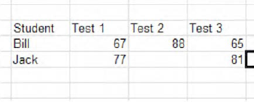
COUNT will thus tell you that Bill has taken 3 exams and Jack has attempted 2, and so needs to make one up. Or, by way of additional example: if you've entered a list of potential donors to a charity on your sheet and key in the amount of each contribution when it's received, you'd use SUM to learn how much money you've taken in to date, and COUNT to let you know how many individuals have donated, by counting each donation. And while you're at it, you could compute the average size of the donations, couldn't you?
But why does Excel advertise COUNT as Count Numbers on its drop-down menu? It does so in order to distinguish COUNT from another function—COUNTA—which counts all the cells in a range that contain any kind of data. Thus for the range shown in (Figure 3-19):

COUNT will return 3, COUNTA 4. (COUNTA, by the way, is written in the same way as COUNT, though it's not included in the above drop-down menu.)
But let's return to the entries in the AutoSum menu. MAX and MIN are almost self-evident; they identify the highest and lowest cells in a range while ignoring blank cells (and text entries), an important omission in these regards. After all, treating blanks as zero could erroneously yield a MIN of zero among a range of other cells—and if you're working with a range consisting entirely of negative numbers, counting a blank cell as zero could yield a MAX of...zero!
And you'll doubtless be able to find a broad niche for MAX and MIN in your spreadsheet doings.
And by way of recapitulation—all the functions assigned a place on the AutoSum drop-down menu are written the same way:
I'm harping on this point because a great many of the other functions in the Excel repertoire display a different syntax, as you'll see.
And while we're talking about SUM, COUNT, AVERAGE and the like, here's another handy but easy-to-miss, hidden-in-plain-sight take on these operations and some more. If you select any set of cells containing numbers (at least two cells, to be exact) and train your gaze on the lower right of the worksheet screen, on what's called the Status Bar, you'll suddenly see a see a mini-report about the data you've highlighted (Figure 3-20):
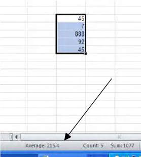
There it is—the Average, Count, and Sum of the range you've selected. Just know that the Count here is really COUNTA; that is, it will count any data in the cell—values, text, and even formulas. What we're presented with here is an on-the-fly summary of the data in the selected range. None of this information will actually appear in the worksheet—and once you move elsewhere to other cells, those figures will change. Still, if you need a quick improvised read on certain data, select that range and take a look.
And what you see there can be customized, at least within limits. If you right-click anywhere on the status bar, you'll trigger a towering short-cut menu, which, among other things, allows you to add three more calculations to the bar (Figure 3-21):

Thus Numerical Count (that is, COUNT), Max, and Min can take their place on the Status Bar too if you need them; simply click them on.
But now that we've gotten our feet wet in the Olympic-sized pool of functions, grab a towel and sit back, because we've some more copying and moving to do, of a different and most important kind.
And in this connection, let's go all the way back to that sample grade-average worksheet I served up in Chapter 1, the one festooned with red highest-score cells and those Sparklines. Don't remember it? I'm not taking it personally—look at Figure 3-22 for a refresher:
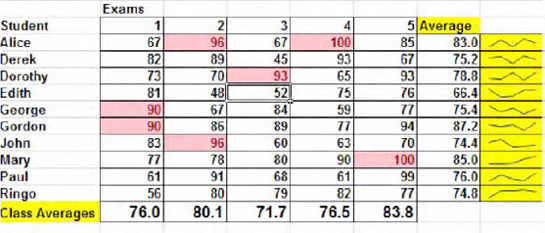
Now look at the Formula Bar. I've clicked cell I10, the one bearing Alice's exam average, and its means of calculation—using AVERAGE, of course—--is recorded up there in that bar. By way of review, we see that Alice's grades occupy range D10:H10 and, by inserting that range reference between AVERAGE's parentheses, we determined her average grade was 83.0.
The point is this: What if I have 150 students in the class (and I've had more than that on occasion), and I need to figure the test average for each and every one of them? Do I have to click the AutoSum button 150 times in order to carry out that disagreeable task?
Yes, that sounds like a rhetorical question, and it is. The answer to it is no, because what we can do instead is copy Alice's AVERAGE formula down the I column for as many rows of students as I need.
Yes, this is a have-to-know, because copying a formula—which entails in essence copying cell references— —is something new—and vital—to the your understanding of how Excel works.
But in fact the ways of actually copying cell references are identical to the ones we described earlier (and we're going to learn an additional one soon); what's different is what happens when you copy them. And that preamble raises a larger point. All the cell copying we've discussed to date and will continue to discuss in this chapter entail copying whatever we enter in a cell—as opposed to what we see in the cell. If I copy Alice's AVERAGE elsewhere, I am most assuredly not copying her average of 83. Rather, I'm copying what I typed in cell I10—the formula that calculated her 83.
The following table enumerates the relationship between the kinds of data I could enter in a cell and what I would see in that cell. In every case, what I would copy is posted in the left column of Table 3-2 below:
Table 3.2. Cell Entries and Cell Displays
Data Example (what you've typed in the cell, which is what gets copied) | What you see in the cell |
|---|---|
3 | 3 |
=4+5 | 9 |
=T3/7 | The result of whatever number you enter in T3 divided by 7 |
=AVERAGE(A4:G4) | The average of all the numbers you've entered in A4 through G4. |
Again, what gets copied is what you've actually typed in the cell. And if you copy any expression which contains a cell reference, what will happen is that the cell references in the destination cells—the cells to which you've copied—will change, corresponding to the distance in either rows or columns from the original cell you've copied.
If I copy the number 1, either 1 or a 100 times, I'll see nothing but 1's in the range to which I've copied. But if I copy this:
=C7
what I'll see depends on where I've copied it. If that =C7 was positioned in cell A2 and I copy it to cell A3, I'll see this in that destination cell:
=C8
By way of a more pertinent example, if I go to cell I10 in our grading worksheet and copy Alice's formula:
=AVERAGE(D10:H10)
down one row to I11—Derek's row—we'll see:
=AVERAGE(D11:H11)
You're probably starting to get the idea. If I were to copy Alice's formula all the way down to say, cell I20000—and there's no reason why I couldn't—I'd see:
=AVERAGE(D20000:H20000)
See what's changed, and what's remained the same? Remember that a cell address comprises a lettered column reference and a number row reference—and when you copy cell references down a column, only the original row references change, commensurate with the distance you've traveled from the original cell. That's because you've moved down rows, and haven't shifted any columns—and the destination results reflect the amount of movement from the source cell reference.
If on the other hand, were I to copy Alice's formula to cell L10, I'd see:
=AVERAGE(G10:K10)
And see why? In this case, I've copied Alice's original formula three columns to the right, such that only the column parts of its cell references—that is, the letters—have changed, again corresponding to the degree of movement from I10. Thus G is three column letters "away" from D, and K is three columns removed from H. And this time there's been no change in the row references—the numbers, because we've copied across columns only, remaining on the same row as Alice's average. We're still on row 10 in this case.
A quick, acronymic way for nailing this row/column movement question is CARD, which stands for: Columns Across, Rows Down. Copy a cell reference across, and the column letters change; copy it down—or up—and the rows numbers change.
In any event, we've encountered a foundational spreadsheet feature—relative references—which describes what happens by default when you copy a cell reference to any other cell. We can see now that if I click on Alice's original AVERAGE formula, I should be able to copy it down the I column for as many rows as I need, confident in the knowledge that, as long as the original formula is correct, I should be able to compute all the other students' averages correctly. Put another way, I need only write AVERAGE once—and then copy it; and so you can see why this tool is so potent.
And note, by the way, that cells can certainly team cell references with simple numeric values; just keep in mind that copying such a cell will only change the cell reference. Thus if I write this:
=D5+7
in cell H2 and copy it down one row, I'll get:
We see, then, that the 7 won't change—only the original D5 will.
And when you need to copy a formula containing cell references down a column or across a row, there's a most expeditious way to do so, by finding a novel use for a tool we already know —the fill handle. To illustrate:
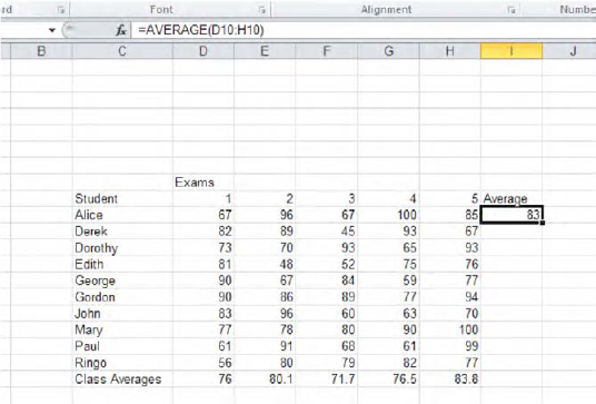
Let's take a few steps back in the design of our grading sheet, and for the sake of clarity, we'll scrub away all the fancy formatting, too. We've written Alice's AVERAGE formula, and now want to copy it down the column, as in Figure 3-23:
If I station my mouse over the fill handle in cell I10—Alice's test average—and then click the handle, don't release the mouse, and drag down the column through Ringo's cell in cell I19 and then release the mouse, I will have copied all the student AVERAGE formulas, as in Figure 3-24:
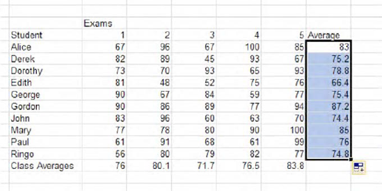
Figure 3.24. Copying allowed, here: Dragging to copy Alice's formula gives me the averages for all the students
Then click anywhere to turn off the blue selection color. Here, the fill handle—that same device we earlier put to the task of producing series of data—e.g., 1,3,5,7, days of the week, etc.—is used to copy formulas. Just click on the first (which at the moment is the only) formula, and drag the fill handle as far as you need to go—either down a column or across a row. The copy procedure collaborates with relative referencing to install the proper cell references in each cell, and what this means is that if you need to copy a formula to many cells, you only need to actually write the formula once—the formula that will serve as the model to be copied to all other cells.
And once you learn how that capability works, there's an even easier and cooler means to carry out this kind of copying task. Once you write that first, model formula, click back on that cell (in this case Alice's average in I10), and double-click the fill handle. All the other student cells running down the I column receive the formula, without you needing to drag the fill handle. The double-click automatically copies the original formula down all the cells that also have data in the immediately adjoining column to its left or right.
To summarize this tip—if you need to copy a formula down a column—and this only works when you copy down a column, not across a row—click on the cell storing the original formula and then double-click its fill handle. As long as there are data in the adjoining column (either to the left or right; and that means in our example if the H column were empty this wouldn't work), the formula copies down for as many rows as there are data. And this will work as surely for 20,000 rows as it will for 20. I use this shortcut all time; I told you I was lazy.
Now there is one more permutation of this cell-reference copying business that you need to know. Consider this case:
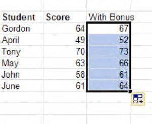
Suppose I've given my students a rather challenging exam, and, after having canvassed the sobering results, decide to grant them an extra three points in order to curve the scores upward. My simple grade book looks like Figure 3-25, at the outset:
So how do I go about padding these pause-giving scores by those three points? Gordon's score is in cell D11, and so I could write the following in E11, couldn't I:
=D11+3
Sure I could. Then I'd return to cell E11, and utilize my newfound double-click-on the fill-handle trick. I'll bring about this revised grade distribution (Figure 3 – 26):
Are my calculations correct? Absolutely; but still I wouldn't recommend this approach. That's because if I conclude that I need to award my charges say, 5 points instead, I'd need to edit the formula in E11 to read:
=D11+5
and then copy that rewritten expression down the column again, so that all the students will enjoy my 5-point largesse. Not an enormously big deal, but not an elegant way in which to proceed. As a rule, one wants to avoid editing cells if one can; it can get messy, and a preferable alternative would be to enter the 5-point bonus figure in a cell—say in this case, A11, and rewrite Gordon's formula thusly:
=D11+A11
and copy it down the column. And exactly why is this approach recommended? Because if I change my mind again and issue a 7-point curve, all I need do is type 7 in cell A11, and all the scores should change automatically—with no additional cell editing required.
But if I go ahead and enter =D11+A11 in Gordon's E11 cell, and once again copy down the E column, I'll see this (Figure 3-27):

Hmmm. That doesn't look quite right, does it? Gordon's score surely exhibits the 5-point increment, but his colleagues seem to have come away with nothing extra at all. What's happened?
What's happened is this: Gordon's bonus-conferring =D11+A11 is correctly written; it references both his test score—64, in D11—and the 5-point give-away, stashed in cell A11. But when I copy this spot-on formula down to April's cell in E12, her formula states:
=D12+A12
and therein lies the problem. Because relative referencing has done its thing, both row numbers in April's formula have pumped to 12, up one from Gordon's 11. And even though cell E12 correctly cites Alice's original test score, cell A12 contains...nothing. And 49 plus nothing... is 49. And that also means that Tony's cell bonus formula—=D13+A13—has to be wrong, too, because A13 is likewise blank, and so on. So apart from Gordon's original bonus calculation all the other students report the wrong bonus result, because they don't reference the cell—A11—in which the bonus is entered. So how is this puzzlement resolved?
Like this. Return to Gordon's cell E11—which remember, contains the correct grade bonus formula —and edit the cell to read:
=D11+A$11
Then copy this revised version down the E column to all the other students. You should now be viewing the correct, bonus-bearing grades for each student. So what's going on? Obviously the dollar sign has something to do with it.
First, we need to understand that the dollar sign has nothing at all to do with currency formatting. Rather, the sign is a programming convention, which freezes the part of the cell address to its immediate right. Installing the dollar sign where we did—alongside the 11 in A11—means that no matter where we copy Gordon's =D11+A$11, that 11 will never change. Thus April's formula now states:
=D12+A$11
and Tony's declares:
=D13+A$11
and soon. Now every student formula reads correctly, because each refers to the same cell containing the grade bonus—A11.
This exercise exemplifies what's called absolute cell referencing, a spreadsheet option in which part of a cell address is held constant, for the kinds of reasons we've just described. It's also certainly possible to place that dollar sign before a column letter, too, if you need to, e.g.:
=$A11
Here the A, or column-referencing segment of the cell address, will never change when it's copied. And if you need to, you can also type:
=$A$11
in which case neither the A nor the 11 will ever change, irrespective of the destination(s) to which they're copied.
Here, then, we've witnessed the potential downside of relative cell referencing. Precisely because relative referencing shifts cell addresses according to their distance from the original, source cell, a series of errant references has crept into our grading process, distorting all our grades save the original, source formula.
And if all these relatives and absolutes are leaving you feeling slightly groggy, you're not alone. This topic is also an acquired taste, and in the early going it takes some doing to acquire it. But give it some thought, play around with it with some mock formulas, and your taste buds should acclimate. With practice they should become second nature to you.
To recapitulate:
You use relative referencing when the same kind of formula needs to be copied down (or across) similar rows or columns of data—such as our grade book example. But of course, the copied formulas can't be identical, because each one needs to calculate a different set of cell references—e.g., Gordon's grades on row 11, April's on row 12, etc.
You'll want—or need—to use an absolute cell reference when different formulas need to reference the same cell repeatedly, e.g., our grade bonus example, where each student's grade adds the point bonus stored in A11.
And what about all those other functions? Excel has hundreds of them; and while you'll be pleased to learn that we don't have room to expound them all, it may be time to recall that bit of unasked-for advice I issued to you about 30 pages ago: namely that it really pays to learn about as many functions as you can.
When I first encountered spreadsheets—in the Paleolithic late 80s, pioneer days when Lotus 1-2-3 ruled the roost and the Undo button was merely a gleam in Bill Gates' eye—my then-boss handed me a rather copious 1-2-3 manual, and wrapped it with one laconic instruction: Learn it. And when I came upon the chapter describing functions—and many of the ones we still use date back to that time—I was incredulous that anyone could actually find a place for these arcane concoctions. But as I learned more about spreadsheets I came to see the wisdom—and the potential value—of a good many of them. In fact, we already know five functions; let's learn some more. Not all of them, mind you, but some important ones—after we learn a few preliminaries.
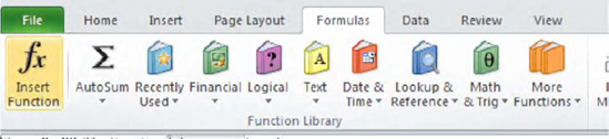
First, you'll want to know that all the Excel functions are neatly catalogued and warehoused inside the buttons shelved in the Function Library group in the Formulas tab (Figure 3-28):
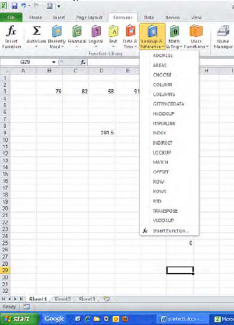
Click one of the buttons, and a directory of functions belonging to the category you clicked drops down, as in Figure 3-28:
Click one of the entries, and you'll be brought to a dialog box whose contents vary by function, but it looks more or less like this (Figure 3-30):
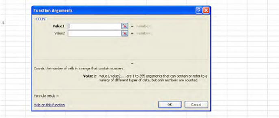
These dialog boxes afford the users a fill-in-the-blanks motif, requesting them to enter essential bits of information, technically called arguments (note the name of the dialog box in Figure 3-28), which when entered enable Excel to calculate the answer you're looking for. Let's look at one such dialog box of a function you already know: see Figure 3-28 for the dialog box for the COUNT function.
What sort of blanks are we asked to fill in here? In this case, ranges. I can type a range in the Value 1 field, or even drag that range on the worksheet itself. Either way the range is recorded in Value 1. If I need to introduce a second range to COUNT, I can identify it in Value 2. And if I need even a third or more ranges, a Value 3, etc., field appears. When I click OK, the COUNT function and result is instated in whichever cell I had clicked before I called up the dialog box.
Remember, though, that the kinds of blanks you'll see in the dialog box will depend on the function you've selected, and you will need to have a pretty good idea what's going on before you can proceed. So if you remain daunted at this point, you can click the Help on this function link in the box's lower left corner; you'll be whisked to a discussion of the function in Excel's Help facility, which is usually pretty clear.
While the buttons in the Function Library afford the most up-front way in which to access functions, Excel makes other ways available, too. You can also click the fx button flanking the Formula Bar to its left and call up this dialog box (Figure 3-31):

In fact, this Insert Function box does nothing more than enumerate the same contents of the respective Library buttons. Click the Or select a category drop-down arrow and you'll see the identical categories by which the Library buttons are classified. Then click a category and any of the function names that appear next, and you'll be returned to exactly the same function Arguments dialog box we witnessed a few screen shots back..
And take note of the Formulas tab's Insert Function button. Click it and, well, you've done nothing more than tap a giant-sized twin of the fx button. Is this button redundant? Probably.
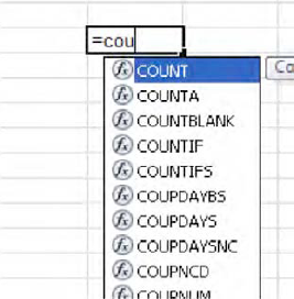
But there is another, decidedly different way to requisition the function you want. Click the cell in which you're working, type =, and begin to enter the function name. As you type, an AutoComplete mechanism activates, presenting and narrowing a list of functions beginning with the letters you've typed. Type more letters and the list shrinks, as shown in Figure 3-32
When you see the one you want, you can either double-click its name, or scroll down to the function in question with the Down arrow key and press Tab (but not Enter). You'll see, for example (Figure 3 – 33):
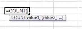
Then start to type the remainder of the functions. True, you'll have to know what to type next, but that's going to come with repetition. (Note the small caption that offers a kind of running commentary about which argument you're currently entering between the parentheses, e.g., which number range you're now identifying in COUNT. But don't worry—more on arguments soon).
The first thing you want to know about functions and formulas (remember that functions are built-in Excel formulas) is that they can be mixed and matched in innumerable ways. They needn't be composed and applied in isolation, and can be related to each other in the same formula, and for a myriad of purposes. So start priming that spreadsheet imagination.
For example, consider this formula:
=AVERAGE(B3:E3)+5
This could, for example, be used to calculate a student's average for four exams (spanning columns B through E), to which 5 points are added—as a kind of bonus.
Now how about this?
=MIN(B3:E3)*1.05
We're working with same four tests. Here our beneficent instructor is adding 5 percent to a student's lowest—that is, minimum—score. Not five points, mind you, but 5 percent. Thus if our student bombed test number 3 with a 58, the above formula will take that score and multiply it by 1.05, coming up with 60.9. Of course, if our teacher is as beneficent as we say, she'll round it up to 61.
Note, by the way, that both of these formulas factor in both a function and an actual, garden-variety number. That's part of Excel's mix-and-match capability.
Now think about this one:
=(SUM(B3:E3)-MIN(B3:E3))/(COUNT(B3:E3)-1)
True, this one looks scary—at least at first, and perhaps even second perusal. But in reality, it doesn't introduce any feature that we haven't already learned. What this formula does is add the scores of all four exams, and subtracts from that total the lowest score. It then divides this new result by the number of remaining exams, that is, 3. In effect the formula calculates the average of the three highest exam scores, having dropped the lowest score.
Let's look at this one more closely—and I'll submit the hope that, upon reflection, you'll agree the formula isn't quite as daunting as you may suppose.
Let's assume our student has scored 76, 82, 58, and 91 on the quartet of exams. Note the entire formula as usual begins with an = sign. But then note that a pair of parentheses surrounds both the SUM and MIN parts of the formula together, this in addition to the parentheses surrounding the individual ranges identified in SUM and MIN. Thus observe the two consecutive parentheses following the B3:E3 range reference in MIN. One simply serves as the closing parenthesis in MIN's own range; the other bounds off the combined SUM-MIN expression, thus letting us compute this total:
76+82+58+91-58
Or 307-58, which equals 249. And why then do we need this pair of global parentheses around SUM and MIN? Because of the order of operations, which assigns priority to expressions surrounded by those parentheses, allowing us to treat the activity going in between them as one unit.
And once we derive it, that 249 is ultimately to be divided by 3—that is, the number of exams minus 1. Now take a look at our divisor:
(COUNT(B3:E3)-1)
And guess what—this expression is also surrounded by parentheses, and for exactly the same reason—the order of operations. Remove those outside parentheses and our divisior would read, formulaically:
COUNT(B3:E3)-1
and numerically:
249/4, then minus 1.
The result: 61.25.
But bring back those outer parentheses and you get:
249/(4-1)
or 83, the number we want.
As a matter of fact, if we peeled off the global parentheses on both sides of the divisor, our formula would stand as:
=SUM(B3:D3)-MIN(B3:D3)/COUNT(B3:D3)-1
And that would yield us 291.5, not even close to the number we want. Try it and you'll see.
Thus writing formulas involves thinking your objectives through, fooling around with practice formulas, making mistakes, and learning from them—and lining up those parentheses when you need them (and Excel will be sure to notify you with an error message when the count of your open parentheses doesn't equal that of your closed ones, something like "Microsoft Excel found an error in the formula you entered," and will offer you a corrected suggestion. Click No to the suggestion and you'll be sent another message, observing that your expression as it stands is missing a parenthesis).
A final note on the above exercise. Even though our formula made important use of the SUM function, we'd probably be advised not to write it and not to click the AutoSum button in order to post it to its cell. And that's because SUM deoesn't stand alone in its cell this time; we needed to continue to type additional characters (incuding that first global parenthesis before the word SUM, which you won't get by clicking AutoSum) in order to combine SUM with the additional formula elements. Just remember, though, that you can always type any function if you need or want to; and in this case, you could type:
=(SUM(
and at that point drag the range B3:E3, continue to type:
)-MIN(
and then drag B3:E3 in order to identify that range for MIN, and continue to type. (And remember that when you begin to type a function name, the Auto Complete menu will appear.)
Now thus far we've confined our discussion of functions to the ones that are presented to us on the AutoSum drop-down menu. But as we stated earlier, there are hundreds more. Time and space will restrict our treatment here to just a few of them, but once you get the general hang of these things, learning additional ones will get that much easier.
Let's start with VLOOKUP, a function I've used countless times to do countless things. The V in VLOOKUP stands for vertical and points to what's called a lookup table, a collection of data in which a value is....looked up.
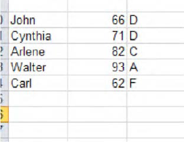
But that's terribly abstract. Let's look at a VLOOKUP example, turning once again to the real-world domain of exam grading. Suppose I've been entrusted with one more batch of grades, to which I assign numerical scores which must be converted into letter grades. In cells K10 through L14, establish the scale shown in Figure 3-34
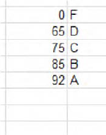
It's a rather simple affair, but notice what the table seems to require, and not to require. The table reads vertically, naturally, and in our case consists of two columns, the first of which records a series of grade intervals which are arrayed in ascending order and aren't evenly spaced in equal numeric intervals—that isn't required.
The second column enumerates the alphabetic grade equivalents, each one of which represents a grade threshold. For example, in order to earn a B you need to achieve a minimum score of 85. Score an 84, and you get a C. Score an 84.9, and you get a C. Tough teacher.
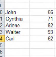
Now we'll enter the scores to be looked up and assigned those alphabet grades. We'll just work with five students, so in cells A10:B14 enter (Figure 3-35):
And it's in the C column, alongside each student grade, in which we'll compose our VLOOKUPs. Click in cell C10 and type:
=VLOOKUP(B10,K$10:L$14,2,TRUE)
Don't worry—we're going to explain all this. First note the constant elements we've spoken about earlier: the equal sign, followed by the function name and an open parenthesis. Second, we see that, unlike say, COUNT or AVERAGE, something more than just a range is fitted in between the parentheses. Here four different elements—or arguments, and we've spoken about them, too—have creeped in there. The first—in this case B10—names the cell whose grade is going to be looked up and assessed. That's John's 66. The second argument—K$10:L$14—pinpoints our lookup range itself, and yes, it's accompanied by those dollar signs, slipped in before the 10 and the 14—the row segments of two cell addresses. And why? Because we want to look up all our students' grades in the same lookup table again and again, and we intend to copy K$10:L$14 down the column of students without its cell references changing.
The third argument—2—refers to the column in the lookup table containing the "answer"—that is, John's alphabetic grade; and so what VLOOKUP does next is this: it takes John's 66 (in B10) and compares it to the numeric grades in the first column of the lookup table—that is, the K column. John's 66 falls between the 65 and the 75 in that column, whereupon VLOOKUP treats it as the lower of these two values (remember—these are grade thresholds, and John hasn't reached 75), and it then looks to see which grade has lined up with 65 in the lookup table's second column—in this case, D. That's the 2 in the third argument. John gets a D, and we can now copy this formula down the C column (using that nifty fill-handle double-click if we wish, because all the cells in the adjoining B column have data in them). The fourth argument—TRUE, which would have been assumed by default anyway even if you hadn't written it—provides for what's called an approximate match. It's this argument which allows VLOOKUP to assess each numeric grade and find its grade niche, e.g., a 78 falls between the lookup table's 75 and 85.
Once done, the student grades should read (Figure 3-36):
and of course this process would enable us to assign the grades of 5000 students, too, not just 5.
And note importantly that the lowest grade we're able to look up in this table is 0 (the entry in K10). Even if it's unlikely that any student will score that poorly, you want your table to be able to handle all contingencies—because had I entered a lowest-possible test score of say, 30, in K10 instead and the hard-partying John crashes and burns with a 25, that score would yield an error message in his VLOOKUP. You can't look up a score below the lowest value in the lookup table.
Let's demonstrate another instance of VLOOKUP, and then review. Suppose we want to calculate some income tax obligations (purely hypothetical, you understand). We can draw up this tax lookup table in cells B8:C18 (Figure 3-37):
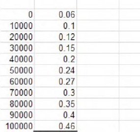
The table presents a tax schedule, which assesses income in dollars, and the values in the second column are really percentages. I haven't formatted either column as currency and percent, respectively, simply because we haven't gotten to formatting yet. Thus an income of $32,567 would be assessed at a rate of .15, or 15%, because that income falls between 30000 and 40000, and again VLOOKUP falls back to the lower of the two and "looks up" the matching figure for 30000 in the second column : .15.
In H8 we can enter any income total, say 62789, and in I8 we can write:
=VLOOKUP(A8,B8:C18,2,TRUE)
Our answer: .27, or 27%.
There's nothing conceptually new in this second case—it's pure review. VLOOKUP takes the number in cell H8-62789—and compares it to the values in the first column of the lookup table in B8:C18. Because the income falls between 60000 and 70000, it's treated as the former, whereupon 60000 is measured against the same row in the second column—namely, .27.
And where are the dollar signs, you ask? You could enter them, and you would, if you had a string of incomes to assess down the H column starting with H8. You'd then copy the original VLOOKUP in I8 down the I column, and yes—here the dollar signs would be most handy indeed, because we'd want all the incomes to be looked up on the same table.
As usual, there's more to say about VLOOKUP. For one thing, if you wanted to learn exactly how much tax a taxpayer actually owes, we could write in cell I8:
=VLOOKUP(A8,B8:C18,2,TRUE)*A8
See how that works? It looks up 62789, yields .27, and goes on to multiply 62789 by .27, returning:
$16,953.03
Once the formatting is applied.
Some other VLOOKUP thoughts: note that our lookup tables to date have comprised two columns. But nothing prevents us from adding a third and even more columns, which would enable us to achieve different sets of lookup outcomes.
For example, I could devise this lookup table, if we return to our grading chores (Figure 3-38):

And we could rewrite John's VLOOKUP in C10 to read:
=VLOOKUP(B10,K$10:M$14,3,TRUE)
In which case we'd see Barely in that cell.
And what's different about this rewrite? Two things: the lookup table now spans three columns, and we're we're looking up our "answer"—the item which will appear in C10—in that third column.
One more VLOOKUP permutation: Suppose we wanted to be able to type a student's name in a selected cell and be able to immediately determine the numeric grade she earned. That is, if I type Cynthia I want to see 71 in the next cell, and so on. If so, we could treat our student name/grade list—A10:B14—as a lookup table. Why not?
And in D10 we could enter any student's name, and in E10 write:
=VLOOKUP(D10,A10:B14,2,FALSE)
I see I can't put anything by you. You've noticed a new, fourth argument in that formula, and here's why.
By default, VLOOKUP requires that the first lookup table coluum—the one containing the values to be looked up and assessed—be arrayed either in ascending numerical or alphabetical order (yes; that first column can display text). But we see that the first column in our current lookup table—the names of students—are assuredly not in such order. If we don't want to sort the list—and here we don't—we can enter FALSE in the VLOOKUP syntax, which instructs Excel to look for exact matches in the first column, irrespective their order—no more approximate matches. So if I type Cynthia in D10, I should see 71 in E10. If I omit the FALSE, I won't see 71 there. And if I type Barack in D10—a name which doesn't appear at all in the lookup table—I'll get an error message.
Again, project this scenario onto 500 or more students, and you'll appreciate how swiftly VLOOKUP can deliver information about any one of them. And before we move on, you'll want to know that VLOOKUP has a sibling named HLOOKUP, which works in precisely the same way, except its lookup table runs horizontally, e.g., (Figure 3-39):

If the table above has been written in say, E13:O24, an HLOOKUP might look like this:
Here a value in cell D3 is looked up in table E13:O14—and the tax percentage—the "answer"—is culled from the second row, not column.
On to another function, one no less valuable—IF. As its name suggests, IF provides a way to sift between (at least) two data alternatives, and to act upon each accordingly. Again, that abstract introduction needs to be exemplified.
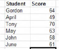
OK. Say I want to be able to award a bonus of $250 to any member of my sales team who exceeds $10,000 in sales in a given month. And suppose I start with this collection of data in cells A5:B8 (Figure 3-40):
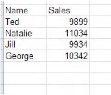
Again, the size of the sales team doesn't really matter—we're just trying to prove the point.
In cell C5—Ted's row—I could write:
=IF(B5>10000,250,0)
And there's your first IF statement. As with VLOOKUP's default, IF requires three arguments:
What's called a logical test—a condition which, if met, makes one thing happen, and if it isn't met, makes something else happen. In our case, the logical test is B5>10000 (note the greater than symbol) and it means, in effect: if the number in cell B5 exceeds 10,000, then...
Value if true. That is, what's going to happen If the condition is met. Again here, if B5 surpasses 10000, the value 250 will be posted in C5—the cell in which I've written the IF statement.
Value if false. What's going to happen if the condition is not met. Here, if the number in B5 falls below 10,000, a zero will be posted in C5—no bonus.
And we can copy this original formula down the C colunn for as many salespersons as we need—and no dollar signs, this time,—because we're assessing a different sales total for each salesperson. We'll see here, of course, that Natalie and George are in line for the $250.
And our Value if true/false consequences can be textual. For example, I could write our statement to read like this:
=IF(B5>10000,"Well Done!","We'll Get 'Em Next Month")
Written this way, one of these declarations will appear in the cells for each salesperson, once it's copied for all. I think they'd prefer the $250, but be that as it may, note that textual if true/false consequences require quotes around them.
And nothing stops you from incorporating other functions into IF, as long as you remember to keep your parentheses in line. Let's get back to Alice, and her 83 test average:
=IF(AVERAGE(D10:H10)>85,"Honor Roll","Nice Try")
If Alice's average were to exceed 85, Honor Roll appears in whatever cell the statement is written. In this case we see that AVERAGE is used here to establish the logical test—and once you've become practiced with nesting functions inside other ones, such as the example we're studying here, you can really start to rock 'n'roll. The data possibilities multiply exponentially.
There's one more function we can squeeze into into this sampler, and this one has real-world pertinence—PMT—short for Payment—a financial formula that can easily tell you how much money you can expect to pay for a mortgage—like it or not.
Stripped to its essentials, PMT has three arguments:
=PMT(rate,nper,pv)
Rate stands for your annual rate, one that will need to be divided by 12, or whatever the payment interval (example coming shortly). Nper signifies the number of payments you need to make across the life of the mortgage, and Pv denotes the present value of the mortgage.
Here's that example: you want to take out a 30-year, $200,000 mortgage at an interest rate of 5.2%. Let's enter these three values in cells B12, C12, and D12, shown in Figure 3-41
(Again, we haven't formatted these values.)
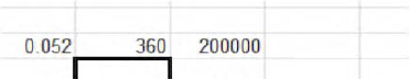
Figure 3.41. The basic three elements needed to write PMT: interest rate, number of payments, and current value of the loan
The .052 is, after all, 5.2%, and the 360 represents 360 monthly payments over 30 years. In E12, type:
=PMT(B12/12,C12,D12)
Note again: it's not obvious, but you need to divide the interest rate by 12 if you pay monthly, as we see above. (Were you to pay semi-monthly you'd have written B12/6—but you'd also be making 180 payments instead, and would have to enter that revised estimate in C12.)
When the smoke clears you should see this in E12:
$1,098.22
You'll note of course that Excel here has automatically formatted our result—by imparting currency features to the figure, as well as daubing the numbers red. Why red? To indicate that you're debiting your account whenever you incur this monthly charge.
Then you can go ahead and write this in any cell you choose:
=E12*C12
That little formula multiplies the monthly debit by 360, the number of times you'll actually have to pay out. Result: $395,359.83, for a $200,000 mortgage at 5.2%. Ouch!
But through the magic of automatic recalcuation, feel free to type in different numbers in any and all of the three cells—B12, C12, or D12. If you can nab a 4.9% rate, you'll pay $1,061,45 instead—37 bucks less a month. Don't spend it all in one place.
If you want to do more with your workbooks than compile data into lists, you need to know at least a bit about how to move your data to the next level—by writing formulas and utilizing Excel's numerous functions, and making something with the information that wasn't there before. In large measure, that's what spreadsheets are about.
As usual, these skills take practice—but again, the more you know about Excel's formula-writing capabilities, the more you can get the data to do what you want them to do, and to tell you what you need to know. And now that we've gotten that message across, let's take a look at the ways in which you can get your spreadsheet message across—by learning how to format your data.