
In this section, we have included three practical data analytics problems with various stages of data-driven activity with R and Hadoop technologies. These data analytics problem definitions are designed such that readers can understand how Big Data analytics can be done with the analytical power of functions, packages of R, and the computational powers of Hadoop.
The data analytics problem definitions are as follows:
- Exploring the categorization of web pages
- Computing the frequency of changes in the stock market
- Predicting the sale price of a blue book for bulldozers (case study)
This data analytics problem is designed to identify the category of a web page of a website, which may categorized popularity wise as high, medium, or low (regular), based on the visit count of the pages. While designing the data requirement stage of the data analytics life cycle, we will see how to collect these types of data from Google Analytics.

As this is a web analytics problem, the goal of the problem is to identify the importance of web pages designed for websites. Based on this information, the content, design, or visits of the lower popular pages can be improved or increased.
In this section, we will be working with data requirement as well as data collection for this data analytics problem. First let's see how the requirement for data can be achieved for this problem.
Since this is a web analytics problem, we will use Google Analytics data source. To retrieve this data from Google Analytics, we need to have an existent Google Analytics account with web traffic data stored on it. To increase the popularity, we will require the visits information of all of the web pages. Also, there are many other attributes available in Google Analytics with respect to dimensions and metrics.
The header format of the dataset to be extracted from Google Analytics is as follows:
date, source, pageTitle, pagePath
date: This is the date of the day when the web page was visitedsource: This is the referral to the web pagepageTitle: This is the title of the web pagepagePath: This is the URL of the web page
As we are going to extract the data from Google Analytics, we need to use RGoogleAnalytics, which is an R library for extracting Google Analytics datasets within R. To extract data, you need this plugin to be installed in R. Then you will be able to use its functions.
The following is the code for the extraction process from Google Analytics:
# Loading the RGoogleAnalytics library
require("RGoogleAnalyics")

# Step 1. Authorize your account and paste the access_token
query <- QueryBuilder()
access_token <- query$authorize()

# Step 2. Create a new Google Analytics API object
ga <- RGoogleAnalytics()

# To retrieve profiles from Google Analytics
ga.profiles <- ga$GetProfileData(access_token)

# List the GA profiles
ga.profiles

# Step 3. Setting up the input parameters
profile <- ga.profiles$id[3]
startdate <- "2010-01-08"
enddate <- "2013-08-23"
dimension <- "ga:date,ga:source,ga:pageTitle,ga:pagePath"
metric <- "ga:visits"
sort <- "ga:visits"
maxresults <- 100099

# Step 4. Build the query string, use the profile by setting its index value
query$Init(start.date = startdate,
           end.date = enddate,
           dimensions = dimension,
           metrics = metric,

           max.results = maxresults,
           table.id = paste("ga:",profile,sep="",collapse=","),
           access_token=access_token)

# Step 5. Make a request to get the data from the API
ga.data <- ga$GetReportData(query)

# Look at the returned data
head(ga.data)
write.csv(ga.data,"webpages.csv", row.names=FALSE)
The preceding file will be available with the chapter contents for download.
Now, we have the raw data for Google Analytics available in a CSV file. We need to process this data before providing it to the MapReduce algorithm.
There are two main changes that need to be performed into the dataset:
- Query parameters needs to be removed from the column
pagePathas follows:pagePath <- as.character(data$pagePath) pagePath <- strsplit(pagePath,"\?") pagePath <- do.call("rbind", pagePath) pagePath <- pagePath [,1] - The new CSV file needs to be created as follows:
data  <- data.frame(source=data$source, pagePath=d,visits =)
write.csv(data, "webpages_mapreduce.csv" , row.names=FALSE)
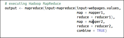
To perform the categorization over website pages, we will build and run the MapReduce algorithm with R and Hadoop integration. As already discussed in the Chapter 2, Writing Hadoop MapReduce Programs, sometimes we need to use multiple Mappers and Reducers for performing data analytics; this means using the chained MapReduce jobs.
In case of chaining MapReduce jobs, multiple Mappers and Reducers can communicate in such a way that the output of the first job will be assigned to the second job as input. The MapReduce execution sequence is described in the following diagram:

Chaining MapReduce
Now let's start with the programming task to perform analytics:
- Initialize by setting Hadoop variables and loading the
rmr2andrhdfspackages of the RHadoop libraries:# setting up the Hadoop variables need by RHadoop Sys.setenv(HADOOP_HOME="/usr/local/hadoop/") Sys.setenv(HADOOP_CMD="/usr/local/hadoop/bin/hadoop") # Loading the RHadoop libraries rmr2 and rhdfs library(rmr2) library(rhdfs) # To initializing hdfs hdfs.init()
- Upload the datasets to HDFS:
# First uploading the data to R console,
webpages <- read.csv("/home/vigs/Downloads/webpages_mapreduce.csv")

# saving R file object to HDFS,
webpages.hdfs <- to.dfs(webpages)
Now we will see the development of Hadoop MapReduce job 1 for these analytics. We will divide this job into Mapper and Reducer. Since, there are two MapReduce jobs, there will be two Mappers and Reducers. Also note that here we need to create only one file for both the jobs with all Mappers and Reducers. Mapper and Reducer will be established by defining their separate functions.
Let's see MapReduce job 1.
- Mapper 1: The code for this is as follows:
mapper1 <- function(k,v) { # To storing pagePath column data in to key object key <- v[2] # To store visits column data into val object Val <- v[3] # emitting key and value for each row keyval(key, val) } totalvisits <- sum(webpages$visits) - Reducer 1: The code for this is as follows:
reducer1 <- function(k,v) { # Calculating percentage visits for the specific URL per <- (sum(v)/totalvisits)*100 # Identify the category of URL if (per <33 ) { val <- "low" } if (per >33 && per < 67) { val <- "medium" } if (per > 67) { val <- "high" } # emitting key and values keyval(k, val) } - Output of MapReduce job 1: The intermediate output for the information is shown in the following screenshot:
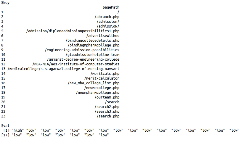
The output in the preceding screenshot is only for information about the output of this MapReduce job 1. This can be considered an intermediate output where only 100 data rows have been considered from the whole dataset for providing output. In these rows, 23 URLs are unique; so the output has provided 23 URLs.
Let's see Hadoop MapReduce job 2:
- Mapper 2: The code for this is as follows:
#Mapper: mapper2 <- function(k, v) { # Reversing key and values and emitting them keyval(v,k) } - Reducer 2: The code for this is as follows:
key <- NA
val <- NULL
# Reducer:
reducer2  <-  function(k, v) {


# for checking whether key-values are already assigned or not.
 if(is.na(key)) {
 key <- k
 val <- v
  } else {
   if(key==k) {
 val <- c(val,v)
  } else{
   key <- k
   val <- v
  }
 }
# emitting key and list of values
keyval(key,list(val))
}
Once we are ready with the logic of the Mapper and Reducer, MapReduce jobs can be executed by the MapReduce method of the rmr2 package. Here we have developed multiple MapReduce jobs, so we need to call the mapreduce function within the mapreduce function with the required parameters.
The command for calling a chained MapReduce job is seen in the following figure:
The following is the command for retrieving the generated output from HDFS:
from.dfs(output)
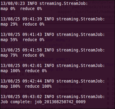
While executing Hadoop MapReduce, the execution log output will be printed over the terminal for the purpose of monitoring. We will understand MapReduce job 1 and MapReduce job 2 by separating them into different parts.
The details for MapReduce job 1 is as follows:
- Tracking the MapReduce job metadata: With this initial portion of log, we can identify the metadata for the Hadoop MapReduce job. We can also track the job status with the web browser by calling the given
Tracking URL.
- Tracking status of Mapper and Reducer tasks: With this portion of log, we can monitor the status of the Mapper or Reducer task being run on Hadoop cluster to get details such as whether it was a success or a failure.

- Tracking HDFS output location: Once the MapReduce job is completed, its output location will be displayed at the end of logs.

For MapReduce job 2.
- Tracking the MapReduce job metadata: With this initial portion of log, we can identify the metadata for the Hadoop MapReduce job. We can also track the job status with the web browser by calling the given
Tracking URL.
- Tracking status of the Mapper and Reducer tasks: With this portion of log, we can monitor the status of the Mapper or Reducer tasks being run on the Hadoop cluster to get the details such as whether it was successful or failed.

- Tracking HDFS output location: Once the MapReduce job is completed, its output location will be displayed at the end of the logs.

The output of this chained MapReduce job is stored at an HDFS location, which can be retrieved by the command:
from.dfs(output)
The response to the preceding command is shown in the following figure (output only for the top 1000 rows of the dataset):

We collected the web page categorization output using the three categories. I think the best thing we can do is simply list the URLs. But if we have more information, such as sources, we can represent the web pages as nodes of a graph, colored by popularity with directed edges when users follow the links. This can lead to more informative insights.
This data analytics MapReduce problem is designed for calculating the frequency of stock market changes.
Since this is a typical stock market data analytics problem, it will calculate the frequency of past changes for one particular symbol of the stock market, such as a Fourier Transformation. Based on this information, the investor can get more insights on changes for different time periods. So the goal of this analytics is to calculate the frequencies of percentage change.

For this stock market analytics, we will use Yahoo! Finance as the input dataset. We need to retrieve the specific symbol's stock information. To retrieve this data, we will use the Yahoo! API with the following parameters:
- From month
- From day
- From year
- To month
- To day
- To year
- Symbol
Tip
For more information on this API, visit http://developer.yahoo.com/finance/.
To perform the analytics over the extracted dataset, we will use R to fire the following command:
stock_BP <- read.csv("http://ichart.finance.yahoo.com/table.csv?s=BP")
Or you can also download via the terminal:
wget http://ichart.finance.yahoo.com/table.csv?s=BP
#exporting to csv file

write.csv(stock_BP,"table.csv", row.names=FALSE)
Then upload it to HDFS by creating a specific Hadoop directory for this:
# creating /stock directory in hdfs
bin/hadoop dfs -mkdir /stock

# uploading table.csv to hdfs in /stock directory
bin/hadoop dfs -put /home/Vignesh/downloads/table.csv /stock/
To perform the data analytics operations, we will use streaming with R and Hadoop (without the HadoopStreaming package). So, the development of this MapReduce job can be done without any RHadoop integrated library/package.
In this MapReduce job, we have defined Map and Reduce in different R files to be provided to the Hadoop streaming function.
- Mapper:
stock_mapper.R#! /usr/bin/env/Rscript # To disable the warnings options(warn=-1) # To take input the data from streaming input <- file("stdin", "r") # To reading the each lines of documents till the end while(length(currentLine <-readLines(input, n=1, warn=FALSE)) > 0) { # To split the line by "," seperator fields <- unlist(strsplit(currentLine, ",")) # Capturing open column value open <- as.double(fields[2]) # Capturing close columns value close <- as.double(fields[5]) # Calculating the difference of close and open attribute change <- (close-open) # emitting change as key and value as 1 write(paste(change, 1, sep=" "), stdout()) } close(input)
- Reducer:
stock_reducer.R#! /usr/bin/env Rscript stock.key <- NA stock.val <- 0.0 conn <- file("stdin", open="r") while (length(next.line <- readLines(conn, n=1)) > 0) { split.line <- strsplit(next.line, " ") key <- split.line[[1]][1] val <- as.numeric(split.line[[1]][2]) if (is.na(current.key)) { current.key <- key current.val <- val } else { if (current.key == key) { current.val <- current.val + val } else { write(paste(current.key, current.val, sep=" "), stdout()) current.key <- key current.val<- val } } } write(paste(current.key, current.val, sep=" "), stdout()) close(conn)
From the following codes, we run MapReduce in R without installing or using any R library/package. There is one system() method in R to fire the system command within R console to help us direct the firing of Hadoop jobs within R. It will also provide the repose of the commands into the R console.
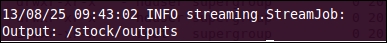
# For locating at Hadoop Directory
system("cd $HADOOP_HOME")

# For listing all HDFS first level directorysystem("bin/hadoop dfs -ls /")

# For running Hadoop MapReduce with streaming parameters
system(paste("bin/hadoop jar
/usr/local/hadoop/contrib/streaming/hadoop-streaming-1.0.3.jar ",

" -input /stock/table.csv",
" -output /stock/outputs",
" -file /usr/local/hadoop/stock/stock_mapper.R",
" -mapper /usr/local/hadoop/stock/stock_mapper.R",
" -file /usr/local/hadoop/stock/stock_reducer.R",
" -reducer /usr/local/hadoop/stock/stock_reducer.R"))

# For storing the output of list command
dir <- system("bin/hadoop dfs -ls /stock/outputs", intern=TRUE)
dir

# For storing the output from part-oooo (output file)
out <- system("bin/hadoop dfs -cat /stock/outputs/part-00000", intern=TRUE)

# displaying Hadoop MapReduce output data out
You can also run this same program via the terminal:
bin/hadoop jar /usr/local/hadoop/contrib/streaming/hadoop-streaming-1.0.3.jar

 -input /stock/table.csv
 -output /stock/outputs
 -file /usr/local/hadoop/stock/stock_mapper.R
 -mapper /usr/local/hadoop/stock/stock_mapper.R
 -file /usr/local/hadoop/stock/stock_reducer.R
 -reducer /usr/local/hadoop/stock/stock_reducer.R
While running this program, the output at your R console or terminal will be as given in the following screenshot, and with the help of this we can monitor the status of the Hadoop MapReduce job. Here we will see them sequentially with the divided parts. Please note that we have separated the logs output into parts to help you understand them better.
The MapReduce log output contains (when run from terminal):
- With this initial portion of log, we can identify the metadata for the Hadoop MapReduce job. We can also track the job status with the web browser, by calling the given
Tracking URL. This is how the MapReduce job metadata is tracked.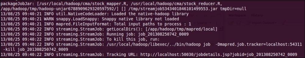
- With this portion of log, we can monitor the status of the Mapper or Reducer tasks being run on the Hadoop cluster to get the details like whether it was successful or failed. This is how we track the status of the Mapper and Reducer tasks.
- Once the MapReduce job is completed, its output location will be displayed at the end of the logs. This is known as tracking the HDFS output location.
- From the terminal, the output of the Hadoop MapReduce program can be called using the following command:
bin/hadoop dfs -cat /stock/outputs/part-00000 - The headers of the output of your MapReduce program will look as follows:
change frequency - The following figure shows the sample output of MapReduce problem:

We can get more insights if we visualize our output with various graphs in R. Here, we have tried to visualize the output with the help of the ggplot2 package.

From the previous graph, we can quickly identify that most of the time the stock price has changed from around 0 to 1.5. So, the stock's price movements in the history will be helpful at the time of investing.
The required code for generating this graph is as follows:
# Loading ggplot2 library
library(ggplot2);

# we have stored above terminal output to stock_output.txt file

#loading it to R workspace
myStockData <- read.delim("stock_output.txt", header=F, sep="", dec=".");

# plotting the data with ggplot2 geom_smooth function
ggplot(myStockData, aes(x=V1, y=V2)) + geom_smooth() + geom_point();
In the next section, we have included the case study on how Big Data analytics is performed with R and Hadoop for the Kaggle data competition.
This is a case study for predicting the auction sale price for a piece of heavy equipment to create a blue book for bulldozers.
In this example, I have included a case study by Cloudera data scientists on how large datasets can be resampled, and applied the random forest model with R and Hadoop. Here, I have considered the Kaggle blue book for bulldozers competition for understanding the types of Big Data problem definitions. Here, the goal of this competition is to predict the sale price of a particular piece of heavy equipment at a usage auction based on its usage, equipment type, and configuration. This solution has been provided by Uri Laserson (Data Scientist at Cloudera). The provided data contains the information about auction result posting, usage, and equipment configuration.
It's a trick to model the Big Data sets and divide them into the smaller datasets. Fitting the model on that dataset is a traditional machine learning technique such as random forests or bagging. There are possibly two reasons for random forests:
- Large datasets typically live in a cluster, so any operations will have some level of parallelism. Separate models fit on separate nodes that contain different subsets of the initial data.
- Even if you can use the entire initial dataset to fit a single model, it turns out that ensemble methods, where you fit multiple smaller models by using subsets of data, generally outperform single models. Indeed, fitting a single model with 100M data points can perform worse than fitting just a few models with 10M data points each (so smaller total data outperforms larger total data).
Sampling with replacement is the most popular method for sampling from the initial dataset for producing a collection of samples for model fitting. This method is equivalent to sampling from a multinomial distribution, where the probability of selecting any individual input data point is uniform over the entire dataset.
For this competition, Kaggle has provided real-world datasets that comprises approximately 4,00,000 training data points. Each data point represents the various attributes of sales, configuration of the bulldozer, and sale price. To find out where to predict the sales price, the random forest regression model needs to be implemented.
Note
The reference link for this Kaggle competition is http://www.kaggle.com/c/bluebook-for-bulldozers. You can check the data, information, forum, and leaderboard as well as explore some other Big Data analytics competitions and participate in them to evaluate your data analytics skills.
We chose this model because we are interested in predicting the sales price in numeric values from random sets of a large dataset.
The datasets are provided in the terms of the following data files:
|
File name |
Description format (size) |
|---|---|
|
|
This is a training set that contains data for 2011. |
|
|
This is a validation set that contains data from January 1, 2012 to April 30, 2012. |
|
|
This is the metadata of the training dataset variables. |
|
|
This contains the correct year of manufacturing for a given machine along with the make, model, and product class details. |
|
|
This tests datasets. |
|
|
This is the benchmark solution provided by the host. |
To perform the analytics over the provided Kaggle datasets, we need to build a predictive model. To predict the sale price for the auction, we will fit the model over provided datasets. But the datasets are provided with more than one file. So we will merge them as well as perform data augmentation for acquiring more meaningful data. We are going to build a model from Train.csv and Machine_Appendix.csv for better prediction of the sale price.
Here are the data preprocessing tasks that need to be performed over the datasets:
# Loading Train.csv dataset which includes the Sales as well as machine identifier data attributes.

transactions <- read.table(file="~/Downloads/Train.csv",
header=TRUE,
sep=",",
quote=""",
row.names=1,
fill=TRUE,
colClasses=c(MachineID="factor",
 ModelID="factor",
datasource="factor",
YearMade="character",
SalesID="character",
auctioneerID="factor",
UsageBand="factor",
saledate="custom.date.2",
Tire_Size="tire.size",
Undercarriage_Pad_Width="undercarriage",
Stick_Length="stick.length"),
na.strings=na.values)

# Loading Machine_Appendix.csv for machine configuration information

machines <- read.table(file="~/Downloads/Machine_Appendix.csv",
header=TRUE,
sep=",",
quote=""",
fill=TRUE,
colClasses=c(MachineID="character",
ModelID="factor",
fiManufacturerID="factor"),
na.strings=na.values)


# Updating the values to numeric
# updating sale data number
transactions$saledatenumeric <- as.numeric(transactions$saledate)
transactions$ageAtSale <- as.numeric(transactions$saledate - as.Date(transactions$YearMade, format="%Y"))

transactions$saleYear <- as.numeric(format(transactions$saledate, "%Y"))

# updating the month of sale from transaction
transactions$saleMonth <- as.factor(format(transactions$saledate, "%B"))

# updating the date of sale from transaction
transactions$saleDay <- as.factor(format(transactions$saledate, "%d"))

# updating the day of week of sale from transaction
transactions$saleWeekday <- as.factor(format(transactions$saledate, "%A"))

# updating the year of sale from transaction
transactions$YearMade <- as.integer(transactions$YearMade)

# deriving the model price from transaction
transactions$MedianModelPrice <- unsplit(lapply(split(transactions$SalePrice,
transactions$ModelID), median), transactions$ModelID)


# deriving the model count from transaction
transactions$ModelCount <- unsplit(lapply(split(transactions$SalePrice, transactions$ModelID), length), transactions$ModelID)

# Merging the transaction and machine data in to dataframe
training.data <- merge(x=transactions, y=machines, by="MachineID")

# write denormalized data out
write.table(x=training.data,
file="~/temp/training.csv",
sep=",",
quote=TRUE,
row.names=FALSE,
eol="
",
col.names=FALSE)
# Create poisson directory at HDFS
bin/hadoop dfs -mkdir /poisson

# Uploading file training.csv at HDFS
bin/hadoop dfs -put ~/temp/training.csv /poisson/
As we are going to perform analytics with sampled datasets, we need to understand how many datasets need to be sampled.
For random sampling, we have considered three model parameters, which are as follows:
- We have N data points in our initial training set. This is very large (106-109) and is distributed over an HDFS cluster.
- We are going to train a set of M different models for an ensemble classifier.
- Each of the M models will be fitted with K data points, where typically K << N. (For example, K may be 1-10 percent of N.).
We have N numbers of training datasets, which are fixed and generally outside our control. As we are going to handle this via Poisson sampling, we need to define the total number of input vectors to be consumed into the random forest model.
There are three cases to be considered:
- KM < N: In this case, we are not using the full amount of data available to us
- KM = N: In this case, we can exactly partition our dataset to produce totally independent samples
- KM > N: In this case, we must resample some of our data with replacements
The Poisson sampling method described in the following section handles all the three cases in the same framework. However, note that for the case KM = N, it does not partition the data, but simply resamples it.
Generalized linear models are an extension of the general linear model. Poisson regression is a situation of generalized models. The dependent variable obeys Poisson distribution.
Poisson sampling will be run on the Map of the MapReduce task because it occurs for input data points. This doesn't guarantee that every data point will be considered into the model, which is better than multinomial resampling of full datasets. But it will guarantee the generation of independent samples by using N training input points.
Here, the following graph indicates the amount of missed datasets that can be retrieved in the Poisson sampling with the function of KM/N:

The grey line indicates the value of KM=N. Now, let's look at the pseudo code of the MapReduce algorithm. We have used three parameters: N, M, and K where K is fixed. We used T=K/N to eliminate the need for the value of N in advance.
- An example of sampling parameters: Here, we will implement the preceding logic with a pseudo code. We will start by defining two model input parameters as
frac.per.modelandnum.models, wherefrac.per.modelis used for defining the fraction of the full dataset that can be used, andnum.modelsis used for defining how many models will be fitted from the dataset.T = 0.1 # param 1: K / N-average fraction of input data in each model 10% M = 50 # param 2: number of models
- Logic of Mapper: Mapper will be designed for generating the samples of the full dataset by data wrangling.
def map(k, v): // for each input data point for i in 1:M // for each model m = Poisson(T) // num times curr point should appear in this sample if m > 0 for j in 1:m // emit current input point proper num of times emit (i, v) - Logic of Reducer: Reducer will take a data sample as input and fit the random forest model over it.
def reduce(k, v):
    fit model or calculate statistic with the sample in v
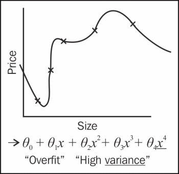
In machine learning, fitting a model means fitting the best line into our data. Fitting a model can fall under several types, namely, under fitting, over fitting, and normal fitting. In case of under and over fitting, there are chances of high bias (cross validation and training errors are high) and high variance (cross validation error is high but training error is low) effects, which is not good. We will normally fit the model over the datasets.
Here are the diagrams for fitting a model over datasets with three types of fitting:


We will fit the model over the data using the random forest technique of machine learning. This is a type of recursive partitioning method, particularly well suited for small and large problems. It involves an ensemble (or set) of classification (or regression) trees that are calculated on random subsets of the data, using a subset of randomly restricted and selected predictors for every split in each classification tree.
Furthermore, the results of an ensemble of classification/regression trees have been used to produce better predictions instead of using the results of just one classification tree.
We will now implement our Poisson sampling strategy with RHadoop. We will start by setting global values for our parameters:
#10% of input data to each sample on avg
frac.per.model <- 0.1
num.models <- 50
Let's check how to implement Mapper as per the specifications in the pseudo code with RHadoop.
- Mapper is implemented in the the following manner:
poisson.subsample <- function(k, input) {
  # this function is used to generate a sample from the current block of data
  generate.sample <- function(i) {
    # generate N Poisson variables
    draws <- rpois(n=nrow(input), lambda=frac.per.model)
    # compute the index vector for the corresponding rows,
    # weighted by the number of Poisson draws
    indices <- rep((1:nrow(input)), draws)
    # emit the rows; RHadoop takes care of replicating the key appropriately
    # and rbinding the data frames from different mappers together for the
    # reducer
    keyval(i, input[indices, ])
  }

  # here is where we generate the actual sampled data
  c.keyval(lapply(1:num.models, generate.sample))
}
Since we are using R, it's tricky to fit the model with the random forest model over the collected sample dataset.
- Reducer is implemented in the following manner:
# REDUCE function fit.trees <- function(k, v) { # rmr rbinds the emitted values, so v is a dataframe # note that do.trace=T is used to produce output to stderr to keep the reduce task from timing out rf <- randomForest(formula=model.formula, data=v, na.action=na.roughfix, ntree=10, do.trace=FALSE) # rf is a list so wrap it in another list to ensure that only # one object gets emitted. this is because keyval is vectorized keyval(k, list(forest=rf)) } - To fit the model, we need
model.formula, which is as follows:model.formula <- SalePrice ~ datasource + auctioneerID + YearMade + saledatenumeric + ProductSize + ProductGroupDesc.x + Enclosure + Hydraulics + ageAtSale + saleYear + saleMonth + saleDay + saleWeekday + MedianModelPrice + ModelCount + MfgYearSalePriceis defined as a response variable and the rest of them are defined as predictor variables for the random forest model. - The MapReduce job can be executed using the following command:
mapreduce(input="/poisson/training.csv",
               input.format=bulldozer.input.format,
               map=poisson.subsample,
               reduce=fit.trees,
               output="/poisson/output")
The resulting trees are dumped in HDFS at
/poisson/output. - Finally, we can load the trees, merge them, and use them to classify new test points:
mraw.forests <- values(from.dfs("/poisson/output"))
forest <- do.call(combine, raw.forests)
Each of the 50 samples produced a random forest with 10 trees, so the final random forest is a collection of 500 trees, fitted in a distributed fashion over a Hadoop cluster.
Note
The full set of source files is available on the official Cloudera blog at http://blog.cloudera.com/blog/2013/02/how-to-resample-from-a-large-data-set-in-parallel-with-r-on-hadoop/.
Hopefully, we have learned a scalable approach for training ensemble classifiers or bootstrapping in a parallel fashion by using a Poisson approximation for multinomial sampling.