2.2.1 Computer Architecture Taxonomy

Before we delve into the details of microprocessor instruction sets, it is helpful to develop some basic terminology. We do so by reviewing a taxonomy of the basic ways we can organize a computer.

A block diagram for one type of computer is shown in Figure 2.1. The computing system consists of a central processing unit (CPU) and a memory. The memory holds both data and instructions, and can be read or written when given an address. A computer whose memory holds both data and instructions is known as a von Neumann machine.

Figure 2.1 A von Neumann architecture computer.

The CPU has several internal registers that store values used internally. One of those registers is the program counter (PC), which holds the address in memory of an instruction. The CPU fetches the instruction from memory, decodes the instruction, and executes it. The program counter does not directly determine what the machine does next, but only indirectly by pointing to an instruction in memory. By changing only the instructions, we can change what the CPU does. It is this separation of the instruction memory from the CPU that distinguishes a stored-program computer from a general finite-state machine.

An alternative to the von Neumann style of organizing computers is the Harvard architecture, which is nearly as old as the von Neumann architecture. As shown in Figure 2.2, a Harvard machine has separate memories for data and program. The program counter points to program memory, not data memory. As a result, it is harder to write self-modifying programs (programs that write data values, then use those values as instructions) on Harvard machines.

Figure 2.2 A Harvard architecture.

Harvard architectures are widely used today for one very simple reason—the separation of program and data memories provides higher performance for digital signal processing. Processing signals in real time places great strains on the data access system in two ways: First, large amounts of data flow through the CPU; and second, that data must be processed at precise intervals, not just when the CPU gets around to it. Data sets that arrive continuously and periodically are called streaming data. Having two memories with separate ports provides higher memory bandwidth; not making data and memory compete for the same port also makes it easier to move the data at the proper times. DSPs constitute a large fraction of all microprocessors sold today, and most of them are Harvard architectures. A single example shows the importance of DSP: Most of the telephone calls in the world go through at least two DSPs, one at each end of the phone call.

Another axis along which we can organize computer architectures relates to their instructions and how they are executed. Many early computer architectures were what is known today as complex instruction set computers (CISC). These machines provided a variety of instructions that may perform very complex tasks, such as string searching; they also generally used a number of different instruction formats of varying lengths. One of the advances in the development of high-performance microprocessors was the concept of reduced instruction set computers (RISC). These computers tended to provide somewhat fewer and simpler instructions. RISC machines generally use load/store instruction sets—operations cannot be performed directly on memory locations, only on registers. The instructions were also chosen so that they could be efficiently executed in pipelined processors. Early RISC designs substantially outperformed CISC designs of the period. As it turns out, we can use RISC techniques to efficiently execute at least a common subset of CISC instruction sets, so the performance gap between RISC-like and CISC-like instruction sets has narrowed somewhat.

Beyond the basic RISC/CISC characterization, we can classify computers by several characteristics of their instruction sets. The instruction set of the computer defines the interface between software modules and the underlying hardware; the instructions define what the hardware will do under certain circumstances. Instructions can have a variety of characteristics, including:

We often characterize architectures by their word length: 4-bit, 8-bit, 16-bit, 32-bit, and so on. In some cases, the length of a data word, an instruction, and an address are the same. Particularly for computers designed to operate on smaller words, instructions and addresses may be longer than the basic data word.

One subtle but important characterization of architectures is the way they number bits, bytes, and words. Cohen [Coh81] introduced the terms little-endian mode (with the lowest-order byte residing in the low-order bits of the word) and big-endian mode (the lowest-order byte stored in the highest bits of the word).

We can also characterize processors by their instruction execution, a separate concern from the instruction set. A single-issue processor executes one instruction at a time. Although it may have several instructions at different stages of execution, only one can be at any particular stage of execution. Several other types of processors allow multiple-issue instruction. A superscalar processor uses specialized logic to identify at run time instructions that can be executed simultaneously. A VLIW processor relies on the compiler to determine what combinations of instructions can be legally executed together. Superscalar processors often use too much energy and are too expensive for widespread use in embedded systems. VLIW processors are often used in high-performance embedded computing.

The set of registers available for use by programs is called the programming model, also known as the programmer model. (The CPU has many other registers that are used for internal operations and are unavailable to programmers.)

There may be several different implementations of an architecture. In fact, the architecture definition serves to define those characteristics that must be true of all implementations and what may vary from implementation to implementation. Different CPUs may offer different clock speeds, different cache configurations, changes to the bus or interrupt lines, and many other changes that can make one model of CPU more attractive than another for any given application.

The CPU is only part of a complete computer system. In addition to the memory, we also need I/O devices to build a useful system. We can build a computer from several different chips but many useful computer systems come on a single chip. A microcontroller is one form of a single-chip computer that includes a processor, memory, and I/O devices. The term microcontroller is usually used to refer to a computer system chip with a relatively small CPU and one that includes some read-only memory for program storage. A system-on-chip generally refers to a larger processor that includes on-chip RAM that is usually supplemented by an off-chip memory.

2.2.2 Assembly Languages

Figure 2.3 shows a fragment of ARM assembly code to remind us of the basic features of assembly languages. Assembly languages usually share the same basic features:

Figure 2.3 An example of ARM assembly language.

Assembly language follows this relatively structured form to make it easy for the assembler to parse the program and to consider most aspects of the program line by line. (It should be remembered that early assemblers were written in assembly language to fit in a very small amount of memory. Those early restrictions have carried into modern assembly languages by tradition.) Figure 2.4 shows the format of an ARM data processing instruction such as an ADD. For the instruction

Figure 2.4 Format of an ARM data processing instruction.

ADDGT r0,r3,#5

the cond field would be set according to the GT condition (1100), the opcode field would be set to the binary code for the ADD instruction (0100), the first operand register Rn would be set to 3 to represent r3, the destination register Rd would be set to 0 for r0, and the operand 2 field would be set to the immediate value of 5.

Assemblers must also provide some pseudo-ops to help programmers create complete assembly language programs. An example of a pseudo-op is one that allows data values to be loaded into memory locations. These allow constants, for example, to be set into memory. An example of a memory allocation pseudo-op for ARM is:

BIGBLOCK  % 10

The ARM % pseudo-op allocates a block of memory of the size specified by the operand and initializes those locations to zero.

2.2.3 VLIW Processors

CPUs can execute programs faster if they can execute more than one instruction at a time. If the operands of one instruction depend on the results of a previous instruction, then the CPU cannot start the new instruction until the earlier instruction has finished. However, adjacent instructions may not directly depend on each other. In this case, the CPU can execute several simultaneously.

Several different techniques have been developed to parallelize execution. Desktop and laptop computers often use superscalar execution. A superscalar processor scans the program during execution to find sets of instructions that can be executed together. Digital signal processing systems are more likely to use very long instruction word (VLIW) processors. These processors rely on the compiler to identify sets of instructions that can be executed in parallel. Superscalar processors can find parallelism that VLIW processors can’t—some instructions may be independent in some situations and not others. However, superscalar processors are more expensive in both cost and energy consumption. Because it is relatively easy to extract parallelism from many DSP applications, the efficiency of VLIW processors can more easily be leveraged by digital signal processing software.

In modern terminology, a set of instructions is bundled together into a VLIW packet, which is a set of instructions that may be executed together. The execution of the next packet will not start until all the instructions in the current packet have finished executing. The compiler identifies packets by analyzing the program to determine sets of instructions that can always execute together.

To understand parallel execution, let’s first understand what constrains instructions from executing in parallel. A data dependency is a relationship between the data operated on by instructions. In the example of Figure 2.5, the first instruction writes into r0 while the second instruction reads from it. As a result, the first instruction must finish before the second instruction can perform its addition. The data dependency graph shows the order in which these operations must be performed.

Figure 2.5 Data dependencies and order of instruction execution.

Branches can also introduce control dependencies. Consider this simple branch

  bnz r3,foo

  add r0,r1,r2

foo: …

The add instruction is executed only if the branch instruction that precedes it does not take its branch.

Opportunities for parallelism arise because many combinations of instructions do not introduce data or control dependencies. The natural grouping of assignments in the source code suggests some opportunities for parallelism that can also be influenced by how the object code uses registers. Consider the example of Figure 2.6. Although these instructions use common input registers, the result of one instruction does not affect the result of the other instructions.

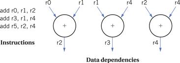
Figure 2.6 Instructions without data dependencies.

VLIW processors examine inter-instruction dependencies only within a packet of instructions. They rely on the compiler to determine the necessary dependencies and group instructions into a packet to avoid combinations of instructions that can’t be properly executed in a packet. Superscalar processors, in contrast, use hardware to analyze the instruction stream and determine dependencies that need to be obeyed.

A number of different processors have implemented VLIW execution modes and these processors have been used in many embedded computing systems. Because the processor does not have to analyze data dependencies at run time, VLIW processors are smaller and consume less power than superscalar processors. VLIW is very well suited to many signal processing and multimedia applications. For example, cellular telephone base stations must perform the same processing on many parallel data streams. Channel processing is easily mapped onto VLIW processors because there are no data dependencies between the different signal channels.