Search in book...
Toggle Font Controls
Create new playlist

Name your new playlist

Playlist description (optional)
Sign In

Email address

Password

Forgot Password?

or

Continue with Facebook

Continue with Google
Sign Up

Full Name

Email address

Confirm Email Address

Password

or

Continue with Facebook

Continue with Google

Chapter 1

Introduction to e-Design

Abstract

The e-Design paradigm employs IT-enabled technology, including virtual prototyping, early in product development to support cross-functional analysis of performance, reliability, and costs, as well as quantitative trade-offs in decision making. Physical prototypes of the product design are then produced using rapid prototyping and computer numerical control. e-Design has the potential to shorten overall product development, improve product quality, and reduce product costs (1) by bringing together product performance, quality, and cost early in the design phase; (2) by supporting design decision making based on quantitative product performance data; and (3) by incorporating physical prototyping to support design verification and functional prototyping. This chapter introduces the e-Design paradigm and the components it comprises, including knowledge-based engineering and virtual and physical prototyping. Designs of a simple airplane engine and a high-mobility multipurpose wheeled vehicle are offered as illustrations.

Keywords

Design trade-off; E-Design; Rapid prototyping; Virtual prototyping

Conventional product development employs a design-build-test philosophy. The sequentially executed development process often results in prolonged lead times and elevated product costs. The proposed e-Design paradigm employs IT-enabled technology for product design, including virtual prototyping (VP) to support a cross-functional team in analyzing product performance, reliability, and manufacturing costs early in product development, and in making quantitative trade-offs for design decision making. Physical prototypes of the product design are then produced using the rapid prototyping (RP) technique and computer numerical control (CNC) to support design verification and functional prototyping, respectively.

e-Design holds potential for shortening the overall product development cycle, improving product quality, and reducing product costs. It offers three concepts and methods for product development:

• Bringing product performance, quality, and manufacturing costs together early in design for consideration.

• Supporting design decision making based on quantitative product performance data.

• Incorporating physical prototyping techniques to support design verification and functional prototyping.

1.1. Introduction

A conventional product development process that is usually conducted sequentially suffers the problem of the design paradox (Ullman 1992). This refers to the dichotomy or mismatch between the design engineer's knowledge about the product and the number of decisions to be made (flexibility) throughout the product development cycle (see Figure 1.1). Major design decisions are usually made in the early design stage when the product is not very well understood. Consequently, engineering changes are frequently requested in later product development stages, when product design evolves and is better understood, to correct decisions made earlier.

Conventional product development is a design-build-test process. Product performance and reliability assessments depend heavily on physical tests, which involve fabricating functional prototypes of the product and usually lengthy and expensive physical tests. Fabricating prototypes usually involves manufacturing process planning and fixtures and tooling for a very small amount of production. The process can be expensive and lengthy, especially when a design change is requested to correct problems found in physical tests.

In conventional product development, design and manufacturing tend to be disjointed. Often, manufacturability of a product is not considered in design. Manufacturing issues usually appear when the design is finalized and tests are completed. Design defects related to manufacturing in process planning or production are usually found too late to be corrected. Consequently, more manufacturing procedures are necessary for production, resulting in elevated product cost.

With this highly structured and sequential process, the product development cycle tends to be extended, cost is elevated, and product quality is often compromised to avoid further delay. Costs and the number of engineering change requests (ECRs) throughout the product development cycle are often proportional according to the pattern shown in Figure 1.2. It is reported that only 8% of the total product budget is spent for design; however, in the early stage, design determines 80% of the lifetime cost of the product (Anderson 1990). Realistically, today's industries will not survive worldwide competition unless they introduce new products of better quality, at lower cost, and with shorter lead times. Many approaches and concepts have been proposed over the years, all with a common goal—to shorten the product development cycle, improve product quality, and reduce product cost.

A number of proposed approaches are along the lines of virtual prototyping (Lee 1999), which is a simulation-based method that helps engineers understand product behavior and make design decisions in a virtual environment. The virtual environment is a computational framework in which the geometric and physical properties of products are accurately simulated and represented. A number of successful virtual prototypes have been reported, such as Boeing's 777 jetliner, General Motors' locomotive engine, Chrysler's automotive interior design, and the Stockholm Metro’s Car 2000 (Lee 1999). In addition to virtual prototyping, the concurrent engineering (CE) concept and methodology have been studied and developed with emphasis on subjects such as product life cycle design, design for X-abilities (DFX), integrated product and process development (IPPD), and Six Sigma (Prasad 1996).

Although significant research has been conducted in improving the product development process and successful stories have been reported, industry at large is not taking advantage of new product development paradigms. The main reason is that small and mid-size companies cannot afford to develop an in-house computer tool environment like those of Boeing and the Big-Three automakers. On the other hand, commercial software tools are not tailored to meet the specific needs of individual companies; they often lack proper engineering capabilities to support specific product development needs, and most of them are not properly integrated. Therefore, companies are using commercial tools to support segments of their product development without employing the new design paradigms to their full advantage.

FIGURE 1.2 Cost/ECR versus time in a conventional design cycle.

The e-Design paradigm does not supersede any of the approaches discussed. Rather, it is simply a realization of concurrent engineering through virtual and physical prototyping with a systematic and quantitative method for design decision making. Moreover, e-Design specializes in performance and reliability assessment and improvement of complex, large-scale, compute-intensive mechanical systems. The paradigm also uses design for manufacturability (DFM), design for manufacturing and assembly (DFMA), and manufacturing cost estimates through virtual manufacturing process planning and simulation for design considerations.

The objective of this chapter is to present an overview of the e-Design paradigm and the sample tool environment that supports a cross-functional team in simulating and designing mechanical products concurrently in the early design stage. In turn, better-quality products can be designed and manufactured at lower cost. With intensive knowledge of the product gained from simulations, better design decisions can be made, breaking the aforementioned design paradox. With the advancement of computer simulations, more hardware tests can be replaced by computer simulations, thus reducing cost and shortening product development time. The desirable cost and ECR distributions throughout the product development cycle shown in Figure 1.3 can be achieved through the e-Design paradigm.

A typical e-Design software environment can be built using a combination of existing computer-aided design (CAD), computer-aided engineering (CAE), and computer-aided manufacturing (CAM) as the base, and integrating discipline-specific software tools that are commercially available for specific simulation tasks. The main technique in building the e-Design environment is tool integration. Tool integration techniques, including product data models, wrappers, engineering views, and design process management, have been developed (Tsai et al. 1995) and are described in Design Theory and Methods using CAD/CAE, a book in The Computer Aided Engineering Design Series. This integrated e-Design tool environment allows small and mid-size companies to conduct efficient product development using the e-Design paradigm. The tool environment is flexible so that additional engineering tools can be incorporated with a lesser effort.

In addition, the basis for tool integration, such as product data management (PDM), is well established in commercial CAD tools and so no wheel needs to be reinvented. The e-Design paradigm employs three main concepts and methods for product development:

• Bringing product performance, quality, and manufacturing cost for design considerations in the early design stage through virtual prototyping.

• Supporting design decision making through a quantitative approach for both concept and detail designs.

• Incorporating product physical prototypes for design verification and functional tests via rapid prototyping and CNC machining, respectively.

In this chapter, the e-Design paradigm is introduced. Then components that make up the paradigm, including knowledge-based engineering (KBE) (Gonzalez and Dankel 1993), virtual prototyping, and physical prototyping, are briefly presented. Designs of a simple airplane engine and a high-mobility multipurpose wheeled vehicle (HMMWV) are briefly discussed to illustrate the e-Design paradigm. Details of modeling and simulation are provided in later chapters.

FIGURE 1.3 (a) Cost/ECR versus e-Design cycle time; (b) product knowledge versus e-Design cycle time.

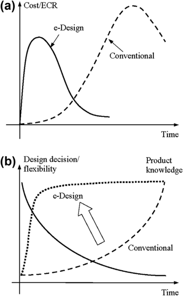
1.2. The e-Design Paradigm

As shown in Figure 1.4, in e-Design, a product design concept is first realized in solid model form by design engineers using CAD tools. The initial product is often established based on the designer's experience and legacy data of previous product lines. It is highly desirable to capture and organize designer experience and legacy data to support decision making in a discrete form so as to realize an initial concept. The KBE (Gonzalez and Dankel 1993) that computerizes knowledge about specific product domains to support design engineers in arriving at a solution to a design problem supports the concept design. In addition, a KBE system integrated with a CAD tool may directly generate a solid model of the concept design that directly serves downstream design and manufacturing simulations.

With the product solid model represented in CAD, simulations for product performance, reliability, and manufacturing can be conducted. The product development tasks and the cross-functional team are organized according to engineering disciplines and expertise. Based on a centralized computer-aided design product model, simulation models can be derived with proper simplifications and assumptions. However, a one-way mapping that governs changes from CAD models to simulation models must be established for rapid simulation model updates (Chang et al. 1998). The mapping maintains consistency between CAD and simulation models throughout the product development cycle.

Product performance, reliability, and manufacturing can then be simulated concurrently. Performance, quality, and costs obtained from multidisciplinary simulations are brought together for review by the cross-functional team. Design variables—including geometric dimensions and material properties of the product CAD models that significantly influence performance, quality, and cost—can be identified by the cross-functional team in the CAD product model. These key performance, quality, and cost measures, as well as design variables, constitute a product design model. With such a model, a systematic design approach, including a parametric study for concept design and a trade-off study for detail design, can be conducted to improve the product with a minimum number of design iterations.

The product designed in the virtual environment can then be fabricated using rapid prototyping machines for physical prototypes directly from product CAD solid models, without tooling and process planning. The physical prototypes support the cross-functional team for design verification and assembly checking. Change requests that are made at this point can be accommodated in the virtual environment without high cost and delay.

The physics-based simulation technology potentially minimizes the need for product hardware tests. Because substantial modeling and simulations are performed, unexpected design defects encountered during the hardware tests are reduced, thus minimizing the feedback loop for design modifications. Moreover, the production process is smooth since the manufacturing process has been planned and simulated. Potential manufacturing-related problems will have been largely addressed in earlier stages.

A number of commercial CAD systems provide a suite of integrated CAD/CAE/CAM capabilities (e.g., Pro/ENGINEER and SolidWorks^®). Other CAD systems, including CATIA^® and NX, support one or more aspects of the engineering analysis. In addition, third-party software companies have made significant efforts in connecting their capabilities to CAD systems. As a representative example, CAE and CAM software companies worked with SolidWorks and integrated their software into SolidWorks environments such as CAMWorks^®. Each individual tool is seamlessly integrated into SolidWorks.

In this book, Pro/ENGINEER and SolidWorks, with a built-in suite of CAE/CAM modules, are employed as the base for the e-Design environment. In addition to their superior solid modeling capability based on parametric technology (Zeid 1991), Pro/MECHANICA^® and SolidWorks Simulation support simulations of nominal engineering, including structural and thermal problems. Mechanism Design of Pro/ENGINEER and SolidWorks Motion support motion simulation of mechanical systems. Moreover, CAM capabilities implemented in CAD, such as Pro/MFG (Parametric Technology Corp., www.ptc.com), and CAMWorks, provide an excellent basis for manufacturing process planning and simulations. Additional CAD/CAE/CAM tools introduced to support modeling and simulation of broader engineering problems encountered in general mechanical systems can be developed and added to the tool environment as needed.

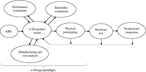
1.3. Virtual Prototyping

Virtual prototyping is the backbone of the e-Design paradigm. As presented in this chapter, VP consists of constructing a parametric product model in CAD, conducting product performance simulations and reliability evaluations using CAE software, and carrying out manufacturing simulations and cost estimates using CAM software. Product modeling and simulations using integrated CAD/CAE/CAM software are the basic and common activities involved in virtual prototyping. However, a systematic design method, including parametric study and design trade-offs, is indispensable for design decision making.

1.3.1. Parameterized CAD Product Model

A parametric product model in CAD is essential to the e-Design paradigm. The product model evolves to a higher-fidelity level from concept to detail design stages (Chang et al. 1998). In the concept design stage, a considerable portion of the product may contain non-CAD data. For example, when the gross motion of the mechanical system is sought, the non-CAD data may include engine, tires, or transmission if a ground vehicle is being designed. Engineering characteristics of the non-CAD parts and assemblies are usually described by engineering parameters, physics laws, or mathematical equations. This non-CAD representation is often added to the product model in the concept design stage for a complete product model. As the design evolves, non-CAD parts and assemblies are refined into solid-model forms for subsystem and component designs as well as for manufacturing process planning.

A primary challenge in conducting product performance simulations is generating simulation models and maintaining consistency between CAD and simulation models through mapping. Challenges involved in model generation and in structural and dynamic simulations are discussed next, in which an airplane engine model in the detail design stage, as shown in Figure 1.5, is used for illustration.

FIGURE 1.5 Airplane engine model: (a) CAD model and (b) model tree.

1.3.1.1. Parameterized product model

A parameterized product model defined in CAD allows design engineers to conveniently explore design alternatives for support of product design. The CAD product model is parameterized by defining dimensions that govern the geometry of parts through geometric features and by establishing relations between dimensions within and across parts. Through dimensions and relations, changes can be made simply by modifying a few dimensional values. Changes are propagated automatically throughout the mechanical product following the dimensions and relations. A single-piston airplane engine with a change in its bore diameter is shown in Figure 1.6, so as illustrating change propagation through parametric dimensions and relationships. More in-depth discussion of the modeling and parameterization of the engine example can be found in Product Design Modeling using CAD/CAE, a book in The Computer Aided Engineering Design Series.

1.3.1.2. Analysis models

For product structural analysis, finite element analysis (FEA) is often employed. In addition to structural geometry, loads, boundary conditions, and material properties can be conveniently defined in the CAD model. Most CAD tools are equipped with fully automatic mesh generation capability. This capability is convenient but often leads to large FEA models with some geometric discrepancy at the part boundary. Plus, triangular and tetrahedral elements are often the only elements supported. An engine connecting rod example meshed using Pro/MESH (part of Pro/MECHANICA) with default mesh parameters is shown in Figure 1.7. The FEA model consists of 1,270 nodes and 4,800 tetrahedron elements, yet it still reveals discrepancy to the true CAD geometry. Moreover, mesh distortion due to large deformation of the structure, such as hyperelastic problems, often causes FEA to abort prematurely. Semiautomatic mesh generation is more realistic; therefore, tools such as MSC/Patran^® (MacNeal-Schwendler Corp., www.mscsoftware.com) and HyperMesh^® (Altair^® Engineering, Inc., www.altair.com) are essential to support the e-Design environment for mesh generation.

FIGURE 1.6 Design change propagation: (a) bore diameter = 1.3 in.; (b) bore diameter changed to 1.6 in.; (c) relations of geometric dimensions.

FIGURE 1.7 Finite element meshes of a connecting rod: (a) CAD solid model, (b) h-version finite element mesh, and (c) p-version finite element mesh.

In general, p-version FEA (Szabó and Babuška 1991) is more suitable for structural analysis in terms of minimizing the gap in geometry between CAD and finite element models, and in lessening the tendency toward mesh distortion. It also offers capability in convergence analysis that is superior to regular h-version FEA. As shown in Figure 1.7c, the same connecting rod is meshed with 568 tetrahedron p-elements, using Pro/MECHANICA with a default setting. A one-way mapping between changes in CAD geometric dimensions and finite element mesh for both h- and p-version FEAs can be established through a design velocity field (Haug et al. 1986), which allows direct and automatic generation of the finite element mesh of new designs.

Another issue worth considering is the simplification of 3D solid models to surface (shell) or curve (beam) models for analysis. Capabilities that semiautomatically convert 3D thin-shell solids to surface models are available in, for example, Pro/MECHANICA and SolidWorks Simulation.

1.3.1.3. Motion simulation models

Generating motion simulation models involves regrouping parts and subassemblies of the mechanical system in CAD as bodies and often introducing non-CAD components to support a multibody dynamic simulation (Haug 1989). Engineers must define the joints or force connections between bodies, including joint type and reference coordinates. Mass properties of each body are computed by CAD with the material properties specified. Integration between Mechanism Design and Pro/ENGINEER, as well as between SolidWorks Motion (Chang 2008) and SolidWorks, is seamless. Design changes made in geometric dimensions propagate to the motion model directly. In addition, simulation tools, such as Dynamic Analysis and Design Systems (DADS) (LMS, www.lmsintl.com/DADS) and communication and data systems integration, are also integrated with CAD with proper parametric mapping from CAD to simulation models that support parametric study. As an example, the motion inside an airplane engine is modeled as a slider-crank mechanism in Mechanism Design, as shown in Figure 1.8.

FIGURE 1.8 Engine motion model: (a) definition and (b) schematic view.

A common mistake made in creating motion simulation models is selecting improper joints to connect bodies. Introducing improper joints creates an invalid or inaccurate model that does not simulate the true behavior of the mechanical system. Intelligent modeling capability that automatically specifies joints in accordance with assembly relations defined between parts and subassemblies in solid models is available in, for example, SolidWorks Motion.

1.3.2. Product Performance Analysis

As mentioned earlier, product performance evaluation using physics-based simulation in the computer environment is usually called, in a narrow sense, virtual prototyping, or VP. With the advancement of simulation technology, more engineering questions can be answered realistically through simulations, thus minimizing the needs for physical tests. However, some key questions cannot be answered for sophisticated engineering problems—for example, the crashworthiness of ground vehicles. Although VP will probably never replace hardware tests completely, the savings it achieves for less sophisticated problems is significant and beneficial.

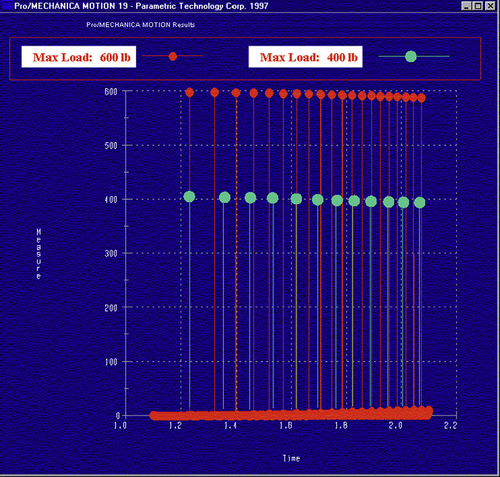
1.3.2.1. Motion analysis

System motion simulations include workspace analysis (kinematics), rigid- and flexible-body dynamics, and inverse dynamic analysis. Mechanism Design and SolidWorks Motion, based on theoretical work (Kane and Levinson 1985), mainly support kinematics and rigid-body simulations for mechanical systems. They do not properly support mechanical system simulation such as a vehicle moving on a user-defined terrain. General-purpose dynamic simulation tools, such as DADS (www.lsmintl.com) or Adams^® (www.mscsoftware.com), are more desirable for simulation of general mechanical systems.

1.3.2.2. Structural analysis

Pro/MECHANICA supports linear static, vibration, buckling, fatigue, and other such analyses, using p-version FEA. General-purpose finite element codes, such as MSC/Nastran^® (MacNeal-Schwendler Corp., www.mscsoftware.com) and ANSYS^® (ANSYS Analysis Systems, Inc., www.ansys.com) are ideal for the e-Design environment to support FEA for a broad range of structural problems—for example, nonlinear, plasticity, and transient dynamics. Meshless methods developed in recent years (for example, Chen et al. 1997) hold promise for avoiding finite element mesh distortion in large-deformation problems. Multiphase problems (e.g., acoustic and aero-structural) are well supported by specialized tools such as LMS^® SYSNOISE (Numerical Integration Technologies 1998). LS-DYNA^® (Hallquist 2006) is currently one of the best codes for nonlinear, plastic, dynamics, friction-contact, and crashworthiness problems. These special codes provide excellent engineering analysis capabilities that complement those provided in CAD systems.

1.3.2.3. Fatigue and fracture analysis

Fatigue and fracture problems are commonly encountered in mechanical components because of repeated mechanical or thermal loads. MSC Fatigue^® (MacNeal-Schwendler Corp., www.mscsoftware.com), with an underlying computational engine developed by nCode^® (www.ncode.com) is one of the leading fatigue and fracture analysis tools. It offers both high- and low-cycle fatigue analyses. A critical plane approach is available in MSC Fatigue for prediction of fatigue life due to general multiaxial loads.

Note that the recently developed extended finite element method (XFEM) supports fracture propagation without re-meshing (Moës et al. 2002). XFEM was recently integrated in ABAQUS^®. Also note that additional capabilities, such as thermal analysis, computational fluid dynamics (CFD) and combustion, can be added to meet specific needs in analyzing mechanical products. Integration of additional engineering disciplines are briefly discussed in Section 1.3.4.

1.3.2.4. Product reliability evaluations

Product reliability evaluations in the e-Design environment focus on the probability of specific failure events (or failure mode). The failure event corresponds to a product performance measure, such as the fatigue life of a mechanical component. For the reliability analysis of a single failure event, the failure event or failure function is defined as (Madsen et al. 1986)

$g (X) = ψ^{u} - ψ (X)$ $g (X) = ψ^{u} - ψ (X)$

(1.1)

where

ψ is a product performance measure

ψ^u is the upper bound (or design requirement) of the product performance

X is a vector of random variables.

When product performance does not meet the requirement—that is, when

ψ^{u} \leq ψ (X)

$ψ^{u} \leq ψ (X)$

, the event fails. Therefore, the probability of failure P_f of the particular event g(X) ≤ 0 is

$P_{f} = P [g (X) \leq 0]$ $P_{f} = P [g (X) \leq 0]$

(1.2)

where P[•] is the probability of event •.

Given the joint probability density function f_X(x) of the random variables X, the probability of failure for a single event of a mechanical component can be expressed as

$P_{f} = P [g (X) \leq 0] = \int \int_{g (X) \leq 0} \dots \int f_{X} (x) d x .$ $P_{f} = P [g (X) \leq 0] = \int \int_{g (X) \leq 0} \dots \int f_{X} (x) d x .$

(1.3)

The probability of failure in Eq. 1.3 is commonly evaluated using the Monte Carlo method or the first- or second-order reliability method (FORM or SORM) (Wu and Wirsching 1984, Yu et al. 1998).

Once the probabilities of several failure events in subsystems or components are computed, system reliability can be obtained by, for example, fault-tree analysis (Ertas and Jones 1993). No general-purpose software tool for reliability analysis of general mechanical systems is commercially available yet. Numerical evaluation of stochastic structures under stress (NESSUS^®) (www.nessus.swri.org), which is currently in development can be a good candidate for incorporation into the e-Design environment. With the probability of failure, critical quality design criteria, such as mean time between failure (MTBF), can be computed (Ertas and Jones 1993).

Two main challenges exist in reliability analysis: One, realistic distribution data are difficult to acquire and often are not available in the early stage; and two, failure probability computations are often expensive. The first challenge may be alleviated by employing legacy data from previous product lines. Approximation techniques (e.g., Yu et al. 1998) can be employed to make the computation affordable even for an individual failure event within a mechanical component.

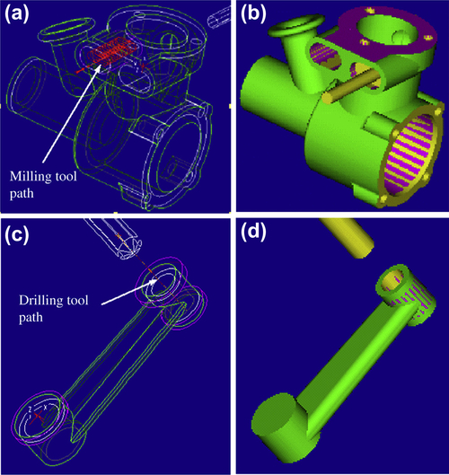
1.3.3. Product Virtual Manufacturing

Virtual manufacturing addresses issues of design for manufacturability (DFM) (Prasad 1996) and design for manufacturing and assembly (DFMA) (Boothroyd et al. 1994) early in product development. In the e-Design paradigm, DFM and DFMA are performed by conducting virtual manufacturing and assembly using, for example, Pro/MFG. DFM and DFMA of the product are verified through animations of the virtual manufacturing and assembly process.

Pro/MFG is a Pro/ENGINEER module supporting the virtual machining process, including milling, drilling, and turning. By incorporating part design and also defining workpieces, workcells, fixtures, cutting tools, and cutting parameters, Pro/MFG automatically generates a toolpath (see Figure 1.9a), which simulates the machining process (Figure 1.9b), calculates machining time, and produces cutter location (CL) data. The CL data can be post-processed for CNC codes. In addition, casting, sheet metal, molding, and welding can be simulated using Pro/CASTING, Pro/SHEETMETAL, Pro/MOLD, and Pro/WELDING, respectively.

With such virtual manufacturing process planning and animation, manufacturability of the product design can, to some extent, be verified. The DFMA tool (Boothroyd et al. 1994) developed by Boothroyd Dewhurst, Inc., assists the cross-functional team in quantifying product assembly time and labor costs. It also challenges the team to simplify product structure, thereby reducing product as well as assembly costs.

One of the limitations in using virtual manufacturing tools (e.g., Pro/MFG) is that chip formation (Fang and Jawahir 1996), a primary consideration in computer numerical control (CNC), is not incorporated into the simulation. In addition, machining parameters, such as power consumption, machining temperature, and tool life, which contribute to manufacturing costs are not yet simulated.

1.3.4. Tool Integration

Techniques developed to support tool integration (Chang et al. 1998) include parameterized product data models, engineering views, tool wrappers, and design process management. Parameterized product data models represent engineering data that are needed for conducting virtual prototyping of the mechanical system. The main sources of the product data model are CAD and non-CAD models. The product data model evolves throughout the product development cycle as illustrated in Figure 1.10.

FIGURE 1.9 Virtual machining process: (a) engine case—milling toolpath; (b) milling simulation; (c) connecting rod—drilling toolpath; (d) drilling simulation.

Engineering views allow engineers from various disciplines to view the product from their own technical perspectives. Through engineering views, engineers create simulation models that are consistent with the product model by simplifying the CAD representation, as needed adding non-CAD product representation and mapping. Tool wrappers provide two-way data translation and transmission between engineering tools and the product data model. Design process management provides the team leader with a tool to monitor and manage the design process. When a new tool of an existing discipline, for example ANSYS for structural FEA, is to be integrated, a wrapper for it must be developed. Three main tasks must be carried out when a new engineering discipline, say computational fluid dynamics (CFD), is added to the environment. First, the product data model must be extended to include engineering data needed to support CFD. Second, engineering views must be added to allow design engineers to generate CFD models. Finally, wrappers must be developed for specific CFD tools.

FIGURE 1.10 Hierarchical product models evolved through the e-Design process.

1.3.5. Design Decision Making

Product performance, reliability, and manufacturing cost that are evaluated using simulations can be brought to the cross-functional team for review. Product performance and reliability are checked against product specifications that have been defined and have evolved from the beginning of the product development process. Manufacturing cost derived from the virtual manufacturing simulations can be added to product cost. The cross-functional team must address areas of concern identified in product performance, reliability, and manufacturability, and it must identify a set of design variables that influence these areas. Design modifications can then be conducted. In the past, quality functional deployment (QFD) (Ertas and Jones 1993) was largely employed in design modification to assign qualitative weighting factors to product performance and design changes. e-Design employes a systematic and quantitative approach to design modifications (for example, Yu et al. 1997).

1.3.5.1. Design problem formulation

Before a design can be improved, design problems must be defined. A design problem is often presented in a mathematical form, typically as

$Minimize φ (b)$ $Minimize φ (b)$

(1.4a)

Subject to

$ψ_{i} (b) \leq ψ_{i}^{u} i = 1, m$ $ψ_{i} (b) \leq ψ_{i}^{u} i = 1, m$

(1.4b)

$P_{f_{j}} (b) \leq P_{f_{j}}^{u} j = 1, n$ $P_{f_{j}} (b) \leq P_{f_{j}}^{u} j = 1, n$

(1.4c)

$b_{k}^{l} \leq b_{k} \leq b_{k}^{u} k = 1, p$ $b_{k}^{l} \leq b_{k} \leq b_{k}^{u} k = 1, p$

(1.4d)

where

φ(b) is the objective (or cost) function to be minimized

ψ_i(b) is the ith constraint function that must be no greater than its upper bound

ψ_{i}^{u}

$ψ_{i}^{u}$

P_{f_j}(b) is the jth failure probability index that must be no greater than its upper bound

P_{f_{j}}^{u}

$P_{f_{j}}^{u}$

b is the vector of design variables

b_k^l and b_k^u are the lower and upper bounds of the design variable b_k, respectively.

Note that in e-Design design variables are usually associated with dimensions of geometric features and part material properties in the parameterized CAD models. The feature-based design parameters serve as the common language to support the cross-functional team while conducting parametric study and design trade-offs.

1.3.5.2. Design sensitivity analysis

Before quantitative design decisions can be made, there must be a design sensitivity analysis (DSA) that computes derivatives of performance measures, including product performance, failure probability, and manufacturing cost, with respect to design variables. Dependence of performance measures on design variables is usually implicit. How to express product performance in terms of design variables in a mathematical form is not straightforward. Analytical DSA methods combined with numerical computations have been developed mainly for structural responses (Haug et al. 1986) and fatigue and fracture (Chang et al. 1997). DSA for failure probability with respect to both deterministic and random variables has also been developed (Yu et al. 1997). In addition, DSA and optimization using meshless methods have been developed for large-deformation problems (Grindeanu et al. 1999). More details about the analytical DSA for structural responses also referred to Haug et al. (1985).

For problems such as motion and manufacturing cost, where premature or no analytical DSA capability is available, the finite difference method is the only choice. The finite difference method is expressed in the following equation:

$\frac{\partial ψ}{\partial b_{j}} \approx \frac{ψ (b + Δ b_{j}) - ψ (b)}{Δ b_{j}}$ $\frac{\partial ψ}{\partial b_{j}} \approx \frac{ψ (b + Δ b_{j}) - ψ (b)}{Δ b_{j}}$

(1.5)

where

Δ b_{j}

$Δ b_{j}$

is a perturbation in the jth design variable. With sensitivity information, parametric study and design trade-offs can be conducted for design improvements at the concept and detail stages, respectively.

1.3.5.3. Parametric study

A parametric study that perturbs design variables in the product design model to explore various design alternatives can effectively support product concept designs. The parametric study is simple and easy to perform as long as the mapping between CAD and simulation models has been established. The mapping supports fast simulation model generation for performance analyses. It also supports DSA using the finite difference method. The parametric study is possible for concept design because the number of design variables to perturb is usually small. A spreadsheet with a proper formula defined among cells is well suited to support the parametric study. The use of Microsoft Excel is illustrated in Figure 1.11.

FIGURE 1.11 Spreadsheet for parametric study and design trade-offs.

1.3.5.4. Design trade-off analysis

With design trade-off analysis, the design engineer can find the most appropriate design search direction for the design problem formulated in Eq. 1.4, using four possible algorithms:

• Reduce cost.

• Correct constraint neglecting cost.

• Correct constraint with a constant cost.

• Correct constraint with a cost increment.

As a general rule, the first algorithm, reduce cost, can be chosen when the design is feasible; in other words, all constraint functions are within the desired limits. When the design is infeasible, generally one may start with the third algorithm, correct constraint with a constant cost. If the design remains infeasible, the fourth algorithm, correct constraint with a cost increment—say 10%—may be appropriate. If a feasible design is still not found, the second algorithm, correct constraint neglecting cost, can be selected. A quadratic programming (QP) subproblem can be formulated to numerically find the search direction that corresponds to the algorithm selected.

FIGURE 1.12 ε-active constraint strategy.

An ε-active constraint strategy (Arora 1989), shown in Figure 1.12, can be employed to support design trade-offs. The constraint functions in Eq. 1.4 are normalized by

$y_{i} = \frac{ψ_{i}}{ψ_{i}^{u}} - 1 \leq 0, i = 1, m$ $y_{i} = \frac{ψ_{i}}{ψ_{i}^{u}} - 1 \leq 0, i = 1, m$

(1.6)

when y_i is between CT (usually 0.03) and CTMIN (usually 0.005), it is active—that is,

ε = | C T | + C T M I N

$ε = | C T | + C T M I N$

, as illustrated in Figure 1.12. When y_i is less than CT, the constraint function is inactive or feasible. When y_i is larger than CTMIN, the constraint function is violated. A QP subproblem can be formulated to find the search direction numerically corresponding to the option selected. For example, the QP subproblem for the first algorithm (cost reduction) can be formulated as

$\begin{matrix} Minimize & c^{T} d + 0.5 d^{T} d \\ Subject & A^{T} d \leq y \\ b^{L} - b^{(k)} \leq d \leq b^{U} - b^{(k)} \end{matrix}$ $\begin{matrix} Minimize & c^{T} d + 0.5 d^{T} d \\ Subject & A^{T} d \leq y \\ b^{L} - b^{(k)} \leq d \leq b^{U} - b^{(k)} \end{matrix}$

(1.7)

where

$c = {[c_{1}, c_{2}, \dots, c_{n 1 + n 2}]}^{T}, c_{i} = \partial φ / \partial b_{i}$ $c = {[c_{1}, c_{2}, \dots, c_{n 1 + n 2}]}^{T}, c_{i} = \partial φ / \partial b_{i}$

d is the search direction to be determined.

$A_{i j} = \partial P_{y_{i}} / \partial b_{j}; b = {[b_{1}, b_{2}, \dots b_{n}]}^{T}$ $A_{i j} = \partial P_{y_{i}} / \partial b_{j}; b = {[b_{1}, b_{2}, \dots b_{n}]}^{T}$

k is the current design iteration.

The objective of the design trade-off algorithm is to find the optimal search direction d under a given circumstance. Details are discussed in Design Theory and Methods using CAD/CAE, a book in The Computer Aided Engineering Design Series.

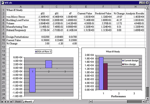
1.3.5.5. What-if study

After the search direction d is found, a number of step sizes α can be used to perturb the design along the direction d. Objective and constraint function values, represented as ψ_i, at a perturbed design b + αd can be approximated using the first-order sensitivity information of the functions by Taylor series expansion about the current design b without going through simulations; that is,

$ψ_{i} (b + α d) \approx ψ_{i} (b) + \frac{\partial ψ_{i}}{\partial b} α d .$ $ψ_{i} (b + α d) \approx ψ_{i} (b) + \frac{\partial ψ_{i}}{\partial b} α d .$

(1.8)

Note that since there is no analysis involved, the what-if study can be carried out very efficiently. This allows the design engineer to explore design alternatives more effectively.

Once a satisfactory design is identified, after trying out different step sizes α in an approximation sense, the design model can be updated to the new design and then simulations of the new design can be conducted. Equation 1.8 also supports parametric study, in which the design perturbation δb is determined by engineers based on sensitivity information. To ensure a reasonably accurate function prediction using Eq. 1.8, the step sizes must be small so that the perturbation

\partial ψ_{i} / (\partial b) (α d)

$\partial ψ_{i} / (\partial b) (α d)$

is, as a rule of thumb, less than 10% of the function value ψ_i(b).

1.4. Physical Prototyping

In general, two techniques are suitable for fabricating physical prototypes of the product in the design process: rapid prototyping (RP) and computer numerical control (CNC) machining. RP systems, based on solid freeform fabrication (SFF) technology (Jacobs 1994), fabricate physical prototypes of the structure for design verification. The CNC machining fabricates functional parts as well as the mold or die for mass production of the product.

1.4.1. Rapid Prototyping

The Solid Freeform Fabrication (SFF) technology, also called Rapid Prototyping (RP), is an additive process that employs a layer-building technique based on horizontal cross-sectional data from a 3D CAD model. Beginning with the bottom-most cross-section of the CAD model, the rapid prototyping machine creates a thin layer of material by slicing the model into so-called 2½ D layers. The system then creates an additional layer on top of the first based on the next higher cross-section. The process repeats until the part is completely built. It is illustrated using an engine case in the example shown in Figure 1.13. Rapid prototyping systems are capable of creating parts with small internal cavities and complex geometry.

Most important, SFF follows the same layering process for any given 3D CAD models, so it requires neither tooling nor manufacturing process planning for prototyping, as required by conventional manufacturing methods. Based on CAD solid models, the SFF technique fabricates physical prototypes of the product in a short turnaround time for design verification. It also supports tooling for product manufacturing, such as mold or die fabrications, through, for example, investment casting (Kalpakjian 1992).

Note that there are various types of SFF systems commercially available, such as the SLA^® 7000 and Sinterstation^® by 3D Systems (Figures 1.14a and 1.14b). In this chapter, the Dimension 1200 sst^® machine (www.stratasys.com), as shown in Figure 1.14c, is presented. More details about it as well as other RP systems will be discussed in Product Manufacturing and Cost Estimating using CAD/CAE, a book in The Computer Aided Engineering Design Series.

FIGURE 1.13 SFF: layered manufacturing: (a) 3D CAD model, (b) 2-1/2D slicing, and (c) physical model.

FIGURE 1.14 Commercial RP systems: (a) 3D systems' SLA 7000, (b) Sinterstation 2500, (c) Stratasys inc.’s dimension 1200 sst. Sources: (b) 3D Systems Corporation, USA; (c) Stratasys Ltd.

FIGURE 1.15 STL engine case models: (a) coarse and (b) refined.

The CAD solid model of the product is first converted into a stereolithographic (STL) format (Chua and Leong 1998), which is a faceted boundary representation uniformly accepted by the industry. Both the coarse and refined STL models of an engine case are shown in Figure 1.15. Even though the STL model is an approximation of the true CAD geometry, increasing the number of triangles can minimize the geometric error effectively. This can be achieved by specifying a smaller chord length, which is defined as the maximum distance between the true geometric boundary and the neighboring edge of the triangle. The faceted representation is then sliced into a series of 2D sections along a prespecified direction. The slicing software is SFF-system dependent.

The Dimension 1200 sst employs fused deposition manufacturing (FDM) technology. Acrylonitrile butadiene styrene (ABS) materials are softened (by elevating temperature), squeezed through a nozzle on the print heads, and laid on the substrate as build and support materials, respectively, following the 2D contours sliced from the 3D solid model (Figure 1.16). Note that various crosshatch options are available in CatalystEX^® software (www.dimensionprinting.com), which comes with the rapid prototyping system.

The physical prototypes are mainly for the cross-functional team to verify the product design and check the assembly. However, they can also be used for discussion with marketing personnel to develop marketing ideas. In addition, the prototypes can be given to potential customers for feedback, thus bringing customers into the design loop early in product development.

1.4.2. CNC Machining

The machining operations of virtual manufacturing, such as milling, turning, and drilling, allow designers to plan the machining process, generate the machining toolpath, visualize and simulate machining operations, and estimate machining time. Moreover, the toolpath generated can be converted into CNC codes (M-codes and G-codes) (Chang et al. 1998, McMahon and Browne 1998) to fabricate functional parts as well as a die or mold for production.

FIGURE 1.16 Crosshatch pattern of a typical cut-out layer: (a) overall and (b) enlarged.

FIGURE 1.17 Cover die machining: (a) virtual and (b) CNC.

For example, the cover die of a mechanical part is machined from an 8 in. × 5.25 in. × 2 in. steel block, as shown in Figure 1.17a. The cutter location data files generated from virtual machining are post-processed into machine control data (MCD)—that is, G- and M-codes, for CNC machining, using post-processor UNCX01.P11 in Pro/MFG. In addition to volume milling and contour surface milling, drilling operations are conducted to create the waterlines. A 3-axis CNC mill, HAAS VF-series (HAAS Automation, Inc. 1996), is employed for fabricating the die for casting the mechanical part (Figure 1.17b).

1.5. Example: Simple Airplane Engine

A single-piston, two-stroke, spark-ignition airplane engine (shown in Figure 1.5) is employed to illustrate the e-Design paradigm and tool environment. The cross-functional team is asked to develop a new model of the engine with a 30% increment in both maximum torque and horsepower at 1,215 rpm. The design of the new engine will be carried out at two interrelated levels: system and component. At the system level, the performance measure is the power output; at the component level, the structural integrity and manufacturing cost of each component are analyzed for improvement. Note that only a very brief discussion is provided in this introductory chapter. The computation and modeling details are discussed in later chapters and Product Design Modeling using CAD/CAE, a book in The Computer Aided Engineering Design Series.

1.5.1. System-Level Design

Power is proportional to the rotational speed of the crankshaft (N), the swept volume (V_s), and the brake mean effective pressure (P_b) (Taylor 1985):

$W_{b} = P_{b} V_{s} N .$ $W_{b} = P_{b} V_{s} N .$

(1.9)

The effective pressure P_b applied on top of the piston depends on, among other factors, the swept volume and the rotational speed of the crankshaft. The pressure is limited by the integrity of the engine structure.

Design variables at the system level include bore diameter (d46:0) and stroke, defined as the distance between the top face of the piston at the bottom and top dead-center positions. In the CAD model, the stroke is defined as the sum of the crank offset length (d6:6) and the connecting rod length (d0:10), as shown in Figure 1.18. To achieve the requirement for system performance, these three design variables are modified as listed in Table 1.1. The design variable values were calculated following theory and practice for internal combustion engines (Taylor 1985). Details of the computation can be found in Silva (2000).

The solid models of the entire engine are automatically updated and properly assembled using the parametric relations established earlier (refer to Figure 1.6b). The change causes P_b to increase from 140 to 180 lbs, so the peak load increases from 400 to 600 lbs. The load magnitude and path applied to the major load-carrying components, such as the connecting rod and crankshaft, are therefore altered. Results from motion analysis show that the system performs well kinematically. Reaction forces applied to the major load-carrying components are computed—for example, for the connecting rod shown in Figure 1.19. The change also affects manufacturing time for some components.

1.5.2. Component-Level Design

Structural performance is evaluated and redesigned to meet the requirements. In addition, virtual manufacturing is conducted for components with significant design changes. Build materials (volume) and manufacturing times constitute a significant portion of the product cost. In this section, the design of the connecting rod is presented to demonstrate the design decision-making method discussed.

Because of the increased load transmitted through the piston and the increased stroke length, the connecting rod can experience buckling failure during combustion. In addition, because changes in stroke length, stiffness, and mass vary, the natural frequency of the rod may be different. Moreover, load is repeatedly applied to the connecting rod, potentially leading to fatigue failure. Structural FEA are conducted to evaluate performance. In addition, virtual manufacturing is carried out to determine the machining cost of the rod.

FIGURE 1.18 Engine assembly with design variables at the system level.

Table 1.1

Changes in Design Variables at the System Level

Design Variable	Current Value (in.)	New Value (in.)	Change (in.)	% Change
Bore diameter (d46:0)	1.416	1.6	0.164	11.6
Crank length (d6:6)	0.5833	0.72	0.1567	26.9
Connecting rod length (d0:10)	2.25	2.49	0.24	10.7

Because of the increment of the connecting rod length (d0:10) and the magnitude of the external load applied (see Figure 1.20), the rod's maximum von Mises stress increases from 13,600 to 18,850 psi and the buckling load factor decreases from 33 to 7. The first natural frequency is 1,515 Hz. The machining time estimated for the connecting rod is 13.2 minutes using hole-drilling and face-milling operations (shown earlier in Figure 1.9d).

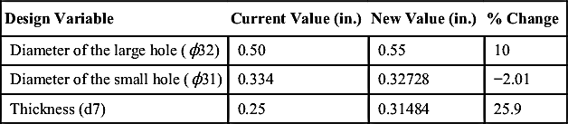
1.5.3. Design Trade-Off

The design trade-off method discussed in Section 1.3.5 is applied to the components, with significant changes resulting from the system-level design. Only the design trade-off conducted for the connecting rod is discussed.

FIGURE 1.19 Dynamic load applied to the connecting rod.

FIGURE 1.20 Engine connecting rod: (a) original design; (b) changes at the system level; (c) changes at the component level.

Table 1.2

Changes in Design Variables at the Component Level

Design Variable	Current Value (in.)	New Value (in.)	% Change
Diameter of the large hole (ϕ32)	0.50	0.55	10
Diameter of the small hole (ϕ31)	0.334	0.32728	−2.01
Thickness (d7)	0.25	0.31484	25.9

Table 1.3

Changes in Performance Measures at the Component Level

Performance Measure	Current Value	New Value	% Change
VM stress	18.9 ksi	10.5 ksi	−44.4
Buckling load factor	7.1	14.2	100
Volume	0.438813 in.³	0.5488 in.³	25.1
Machining time	13.2 min	13.2 min	0
Natural frequency	1515 Hz	1840 Hz	21.5

Performance measures for the connecting rod, including buckling load factor, fatigue life, natural frequency, volume, and machining costs (time), are brought together for design trade-off. Three design variables, ϕ32, ϕ31, and d7, are identified, as shown in Figure 1.20b. The objective is to minimize volume and manufacturing time subject to maximum allowable von Mises stress, operating frequency, and minimum allowable buckling load factor. The engine is designed to work at 21 kHz, and the minimum allowable buckling load factor for the connecting rod is assumed to be 10.

Sensitivity coefficients for performance and cost measures with respect to design variables are calculated (refer to Figure 1.11) using the finite difference method. Design trade-offs are conducted followed by a what-if study. When a satisfactory design is found, the solid model of the rod is updated for performance evaluation and virtual manufacturing. This process is repeated twice when all the requirements are met. The design change is summarized in Tables 1.2 and 1.3, which show that the machining time is maintained and a small volume increment is needed to achieve the required performance.

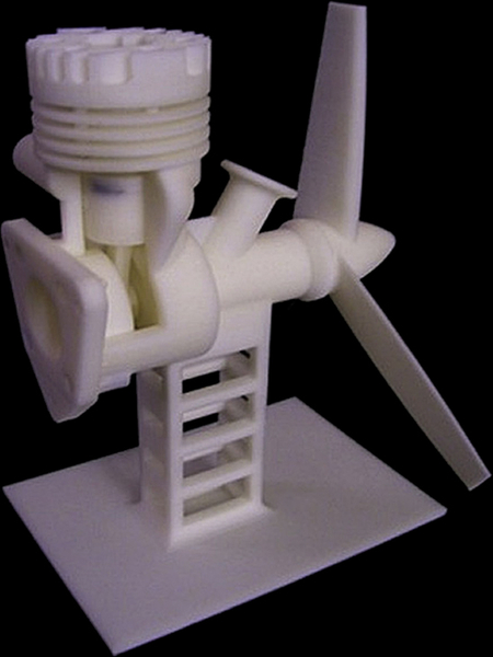
1.5.4. Rapid Prototyping

When the design is finalized through virtual prototyping, rapid prototyping is used to fabricate a physical prototype of the engine, as shown in Figure 1.21. The prototype can be used for design verification as well as tolerance and assembly checking.

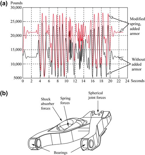
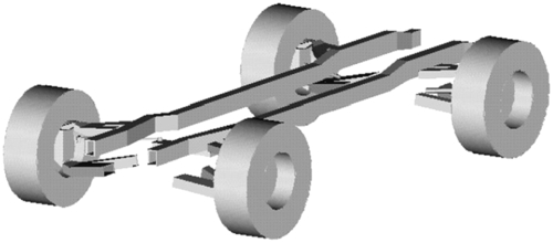
1.6. Example: High-Mobility Multipurpose Wheeled Vehicle

The overall objective of the high-mobility multipurpose wheeled vehicle (HMMWV) design is to ensure that the vehicle's suspension is durable and reliable after accommodating an additional armor loading of 2,900 lb. A design scenario using a hierarchical product model (see Figure 1.10) that evolves during the design process is presented in this section.

FIGURE 1.21 Physical prototypes of engine parts.

In the preliminary design stage, vehicle motion is simulated and design changes are performed to improve the vehicle's gross motion. At this stage, the dynamic behavior of the HMMWV's suspension is simulated and designed. The specific objectives of the preliminary design are to avoid the problem of metal-to-metal contact in the shock absorber due to added armor load, and to improve the driver's comfort by reducing vertical acceleration at the HMMWV driver's seat.

By modifying the spring constant to improve the HMMWV suspension design at the preliminary design stage, the load path generated in HMMWV dynamics simulation is affected in the suspension unit. In the detail design stage, the objective is to assess and redesign the durability, reliability, and structural performance of selected suspension components affected by the added armor load that result in changes in load path and load magnitude.

Note that only a very brief discussion is provided in this introductory chapter. The computation and modeling details are discussed in later chapters.

1.6.1. Hierarchical Product Model

In this particular case, a hierarchical product model is employed to support the HMMWV's design. In all models, nonsuspension parts, such as instrument panel, seats, and lights, are not modeled. Important vehicle components, such as engine and transmission, are modeled using engineering parameters without depending on CAD representation. A low-fidelity CAD model consisting of 18 parts (Figure 1.22) is created using Pro/ENGINEER to support the preliminary design. This model has accurate joint definition and fairly accurate mass property, but less accurate geometry. The goal of the low-fidelity model is to support vehicle dynamic simulation. It is created using substantially less effort compared to that required for the detailed model.

The detailed product model, consisting of more than 200 parts and assemblies (Figure 1.23), is created to support the detail design of suspension components. The detailed model is derived from the preliminary model by (1) breaking an entity into more parts and assemblies (e.g., the gear hub assembly, shown in Figure 1.24) to simulate and design detailed parts, and (2) refining the geometry of mechanical components to support structural FEA (e.g., the lower control arm, shown in Figure 1.25).

FIGURE 1.22 HMMWV CAD model for preliminary design.

FIGURE 1.23 HMMWV CAD model for detail design.

1.6.2. Preliminary Design

The HMMWV is driven repeatedly on a virtual proving ground, as shown in Figure 1.26, with a constant speed of 20 MPH for a period of 23 seconds. A dynamic simulation model, shown in Figure 1.27, is first derived from the low-fidelity CAD solid model of the HMMWV (refer to Figure 1.22). A more in-depth discussion of the HMMWV vehicle dynamic model is provided in Chapter 3.

Using DADS, severe metal-to-metal contact is identified within the shock absorber, caused by the added armor load and rough driving conditions, as shown in Figure 1.28. The spring constant is adjusted to avoid any contact problems; it is increased in proportion to the mass increment of the added armor to maintain the vehicle's natural frequency. This design change not only eliminates the contact problem (see Figure 1.28) but also reduces the amplitude of vertical acceleration at the driver's seat, which improves driving comfort (see Figure 1.29). However, the change alters the load path in the components of the suspension subsystem—for example, the shock absorber force acting on the control arm increases about 75%, as shown in Figure 1.30.

FIGURE 1.24 HMMWV gear hub assembly models: (a) preliminary and (b) detailed.

FIGURE 1.25 HMMWV lower control arm models: (a) preliminary and (b) detailed.

1.6.3. Detail Design

Simulations are carried out for fatigue, vibration, and buckling of the lower control arm (Figure 1.30); reliability of gears in the gear hub assembly (refer to Figure 1.24b); the spring of the shock absorber (see Figure 1.23); and the bearings of the control arm (see Figure 1.30).

Using ANSYS, the first natural frequency of the lower control arm is obtained as 64 Hz, which is far away from vehicle vibration frequency, eliminating concern about resonance. The buckling load factor is analyzed using the peak load at time 10.05 seconds in the 23-second simulation period. The result shows that the control arm will not buckle even under the most severe load. Therefore, the current design is acceptable as far as buckling and resonance of the lower control arm are concerned.

Results obtained from fatigue analyses show that fatigue life (crack initiation) of the lower control arm degrades significantly—for example, from 6.61E+09 to 1.79E+07 blocks (one block is 20 seconds) at critical areas (see Figure 1.31b)—because of the additional armor load and change of load path. Therefore, the design must be altered to improve control arm durability. Reliability of the bearing, gear, and spring at a 99% fatigue failure rate is 2.18E+07, 3.36E+06, and 1.27E+02 blocks, respectively. Note that the fatigue life of the spring at the required reliability is not desirable.

FIGURE 1.28 Shock absorber operation distance (in inches).

FIGURE 1.29 HMMWV driver seat vertical accelerations (in./sec²).

1.6.4. Design Trade-Off

Eleven design parameters, including geometric dimensions (d1 and d2 in Figure 1.32a), material property (cyclic strength coefficient K′ of the lower control arm), and thickness of the control arm sheet metal (t1 to t7 in Figure 1.32b) are defined to support design modification.

FIGURE 1.30 History of shock absorber forces (lbs): (a) force history with and without added armor load, (b) locations of force application.

FIGURE 1.31 HMMWV lower control arm models: (a) finite element and (b) fatigue life prediction.

FIGURE 1.32 Design parameters defined for the control arm: (a) suspension geometric dimensions and (b) thickness dimensions.

A global design trade-off that involves changes in more than one component is conducted first. Geometric design parameters d1 and d2 are modified to reduce loads applied to the control arm, bearing, spring, and gears in the gear hub so that the durability and reliability of these components can be improved. Changes in d1 and d2 affect not only the lower control arm but also the upper control arm and the chassis frame. Sensitivity coefficients of loads at discretized time steps (a total of 10 selected time steps) with respect to parameters d1 and d2 are calculated using a finite difference method. Sensitivity coefficients can be displayed in bar charts (see Figure 1.33a) to guide design modifications. A what-if study is carried out with a design perturbation of 0.6 and 0.3 in. for d1 and d2, respectively, to obtain a reduction in loads. An example of the what-if results is shown in Figure 1.33b.

A local design trade-off that involves design parameters of a single component is carried out for the lower control arm. Thickness design parameters t1 to t7 and the material design parameter K′ are modified to increase the control arm's fatigue life. Fatigue life at ten nodes of its finite element model in the critical area is measured. Sensitivity coefficients of control arm fatigue life at these nodes with respect to the thickness and material parameters are calculated. A design trade-off method using a QP algorithm is employed because of the large number of design parameters and performance measures involved. An improved design obtained shows that with a 0.6% weight increment, fatigue life at the critical area increases about ten times: from 1.79 E+07 to 1.68 E+08 blocks.

FIGURE 1.33 Sensitivity of load on the spherical joint of control arm w.r.t d2 at 10 time steps (a) design sensitivity display and (b) what-if study.

A dynamic simulation is performed again with the detailed model and modified design to ensure that the metal contact problem, encountered in the preliminary design stage, is eliminated as a result of model refinement and design changes in the detail design stage. The global design trade-off reduces the load applied to the shock absorber spring. This reduction significantly increases the spring fatigue life to the desired level.

1.7. Summary

In this chapter, the e-Design paradigm and software tool environment were discussed. The e-Design paradigm employs virtual prototyping for product design and rapid prototyping and computer numerical control (CNC) for fabricating physical prototypes of a design for design verification and functional tests. The e-Design paradigm offers three unique features:

• The VP technique, which simulates product performance, reliability, and manufacturing costs; and brings these measures to design.

• A systematic and quantitative method for design decision making for the parameterized product in solid model forms.

• RP and CNC for fabricating prototypes of the design that verify product design and bring marketing personnel and potential customers into the design loop.

The e-Design approach holds potential for shortening the overall product development cycle, improving product quality, and reducing product costs. With intensive knowledge of the product gained from simulations, better design decisions can be made, thereby overcoming what is known as the design paradox. With the advancement of computer simulations, more hardware tests can be replaced by them, reducing cost and shortening product development time. Manufacturing-related issues can be largely addressed through virtual manufacturing in early design stages. Moreover, manufacturing process planning conducted in virtual manufacturing streamlines the production process.

Questions and Exercises

1.1. In this assignment, you are asked to search and review articles (such as in Mechanical Engineering magazine) that document successful stories in industry that involve employing the e-Design paradigm and/or employing CAD/CAE/CAM technology for product design.

• Briefly summarize the company's history and its main products.

• Briefly summarize the approach and process that the company adopted for product development in the past.

• Why must the company make changes? List a few factors.

• Which approach and process does the company currently employ?

• What is the impact of the changes to the company?

• In which journal, magazine, or website was the article published?

1.2. In this chapter we briefly discussed rapid prototyping technology and the Dimension 1200 sst machine. The sst uses fused deposition manufacturing technology for support of layer manufacturing. Search and review articles to understand the FDM technology and machines that employ such technology other than the Dimension series.

..................Content has been hidden....................

You can't read the all page of ebook, please click here login for view all page.

Table of Contents for Chapter 1. Introduction to e-Design

Create new playlist

Sign In

Sign Up

Abstract

Keywords

1.1. Introduction

1.2. The e-Design Paradigm

1.3. Virtual Prototyping

1.3.1. Parameterized CAD Product Model

1.3.1.1. Parameterized product model

1.3.1.2. Analysis models

1.3.1.3. Motion simulation models

1.3.2. Product Performance Analysis

1.3.2.1. Motion analysis

1.3.2.2. Structural analysis

1.3.2.3. Fatigue and fracture analysis

1.3.2.4. Product reliability evaluations

1.3.3. Product Virtual Manufacturing

1.3.4. Tool Integration

1.3.5. Design Decision Making

1.3.5.1. Design problem formulation

1.3.5.2. Design sensitivity analysis

1.3.5.3. Parametric study

1.3.5.4. Design trade-off analysis

1.3.5.5. What-if study

1.4. Physical Prototyping

1.4.1. Rapid Prototyping

1.4.2. CNC Machining

1.5. Example: Simple Airplane Engine

1.5.1. System-Level Design

1.5.2. Component-Level Design

1.5.3. Design Trade-Off

1.5.4. Rapid Prototyping

1.6. Example: High-Mobility Multipurpose Wheeled Vehicle

1.6.1. Hierarchical Product Model

1.6.2. Preliminary Design

1.6.3. Detail Design

1.6.4. Design Trade-Off

1.7. Summary

Questions and Exercises

Table of Contents for
Chapter 1. Introduction to e-Design

References

Anderson D.M. Design for Manufacturability: Optimizing Cost, Quality, and Time to Market. CIM Press; 1990.
Arora J.S. Introduction to Optimal Design. McGraw-Hill; 1989.
Boothroyd G, Dewhurst P, Knight W. Product Design for Manufacturing and Assembly. Marcel Dekker; 1994.
Chang K.H, Choi K.K, Wang J, Tsai C.S, Hardee E. A multi-level product model for simulation-based design of mechanical systems. Concurrent Engineering Research and Application (CERA) Journal. 1998;6(2):131–144.
Chang K.H, Yu X, Choi K.K. Shape design sensitivity analysis and optimization for structural durability. International Journal of Numerical Methods in Engineering. 1997;40:1719–1743.
Chang T.C, Wysk R.A, Wang H.P. Computer-Aided Manufacturing. second ed. Prentice Hall; 1998.
Chen J.S, Pan C, Wu T.C. Large deformation analysis of rubber based on a reproducing kernel particle method. Computational Mechanics. 1997;19:153–168.
Chua C.K, Leong K.F. Rapid Prototyping: Principles and Applications in Manufacturing. John Wiley; 1998.
Ertas A, Jones J.C. The Engineering Design Process. John Wiley; 1993.
Fang X.D, Jawahir I.S. A hybrid algorithm for predicting chip form/chip breakability in machining. International Journal of Machine Tools and Manufacture. 1996;36(10):1093–1107.
Gonzalez A.J, Dankel D.D. The Engineering of Knowledge-Based Systems, Theory and Practice. Prentice Hall; 1993.
Grindeanu I, Choi K.K, Chen J.S, Chang K.H. Design sensitivity analysis and optimization of hyperelastic structures using a meshless method. AIAA Journal. 1999;37(8):990–997.
HAAS Automation Inc.. VF Series Operations Manual. 1996.
Hallquist J.O. LS-DYNA3D Theory Manual. Livermore Software Technology Corp; 2006.
Haug E.J, Choi K.K, Komkov V. Design Sensitivity Analysis of Structural Systems. Academic Press; 1986.
Haug E.J. Computer-Aided Kinematics and Dynamics of Mechanical Systems, vol. I: Basic Methods. Allyn and Bacon; 1989.
Jacobs P.F. StereoLithography and Other RP&M Technologies. ASME Press; 1994.
Kalpakjian S. Manufacturing Engineering and Technology. second ed. Addison-Wesley; 1992.
Kane T.R, Levinson D.A. Dynamics: Theory and Applications. McGraw-Hill; 1985.
Lee W. Principles of CAD/CAM/CAE Systems. Addison-Wesley Longman; 1999.
Madsen H.O, Krenk S, Lind N.C. Methods of Structural Safety. Prentice Hall; 1986.
McMahon C, Browne J. CADCAM. second ed. Addison-Wesley; 1998.
Moës N, Gravouil A, Belytschko T. Nonplanar 3D crack growth by the extended finite element and level sets. Part I: Mechanical model. International Journal for Numerical Methods in Engineering. 2002;53(11):2549–2568.
Numerical Integration Technologies. SYSNOISE 5.0. 1998.
Prasad B. Concurrent Engineering Fundamentals, vols. I and II: Integrated Product and Process Organization. Prentice Hall; 1996.
Silva J. Concurrent Design and Manufacturing for Mechanical Systems MS thesis. University of Oklahoma; 2000.
Szabó B, Babuška I. Finite Element Analysis. John Wiley; 1991.
Taylor C. The Thermal-Combustion Engine in Theory and Practice, vol. I: Thermodynamics, Fluid Flow, Performance. second ed. MIT Press; 1985.
Tsai C.S, Chang K.H, Wang J. Integration infrastructure for a simulation-based design environment, Proceedings, Computers in Engineering Conference and the Engineering Data Symposium. ASME Design Theory and Methodology Conference. 1995.
Ullman D.G. The Mechanical Design Process. McGraw-Hill; 1992.
Wu Y.T, Wirsching P.H. Advanced reliability method for fatigue analysis. Journal of Engineering Mechanics. 1984;110:536–563.
Yu X, Chang K.H, Choi K.K. Probabilistic structural durability prediction. AIAA Journal. 1998;36(4):628–637.
Yu X, Choi K.K, Chang K.H. A mixed design approach for probabilistic structural durability. Journal of Structural Optimization. 1997;14:81–90.
Zeid I. CAD/CAM Theory and Practice. McGraw-Hill; 1991.
Sources
Dimension sst: www.stratasys.com
HAAS VF-Series: www.haascnc.com
LS-DYNA: www.lstc.com
MSC/Nastran, MSC/Patran: www.mscsoftware.com
Pro/ENGINEER, Pro/MECHANICA, Pro/MFG, Pro/SHEETMETAL, Pro/WELDING, etc.: www.ptc.com
SLA-7000, Sinterstation: www.3dsystems.com
SolidWorks Motion, SolidWorks Simulation: www.solidworks.com