
2.4. Utility Theory
In Sections 2.3.3 and 2.3.4, we used an expected value rule to support decision making under risk and uncertainty. In many situations, it is highly desired that a decision maker's preference is incorporated. Utility theory offers rigorous mathematical framework, within which we are able to examine the preferences of individuals and incorporate them into decision making. In this section, we discuss utility theory from a design perspective. We discuss basics of the theory, including assumptions that lead to axioms of the theory, the utility functions that capture an individual's attitude toward risk, and the construction of utility functions for single and multiple attributes. In the context of design, the attributes are design criteria or design objectives to attain.
2.4.1. Basic Assumptions
There are four assumptions that lead to basic axioms of the utility theory. The first and perhaps the biggest assumption to be made is that any two possible outcomes resulting from a decision can be compared. Given any two possible outcomes, the decision maker can say which one he or she prefers. In some cases, the decision maker can say that they are equally desirable or undesirable. A reasonable extension of the existence of one's preference among outcomes is that the preference is transitive; that is, if one prefers A to B and B to C, then it follows that one prefers A to C.

The second assumption, originated by von Neumann and Morgenstern (von Neumann and Morgenstern 1947), forms the core of modern utility theory. This assumption states that one can assign preferences in the same manner to lotteries involving prizes as one can to the prizes themselves. The lottery gives the probability of one getting prize A is p, and the probability that one gets prize B is 1 − p. Such a lottery is donated as (p, A; 1 − p, B), as represented in Figure 2.7, in which p is between 0 and 1. In utility theory, uncertainty is modeled through lotteries.
Now suppose one is asked to state his or her preferences for prize A, prize B, and a lottery of the above type (p, A; 1 − p, B). Let us assume one prefers prize A to prize B. Then, based on von Neumann and Morgenstern, one would prefer prize A to the lottery (p, A; 1 − p, B) because there is a probability 1 − p that one would be getting the inferior prize B of the lottery. One would also prefer the lottery (p, A; 1 − p, B) to prize B for all probabilities p between 0 and 1. In other words, one would rather have the preferred prize A than the lottery, and one would rather have the lottery than the inferior prize B. Furthermore, it seems logical that, given a choice between two lotteries involving prizes A and B, one would choose the lottery with the higher probability of getting the preferred prize A. That is, one prefers lottery (p, A; 1 − p, B) to (p′, A; 1 − p′, B) if and only if p is greater than p′.
The third assumption is that one's preferences are not affected by the way in which the uncertainty is resolved, bit by bit, or all at once. To illustrate the assumption, let us consider a compound lottery—a lottery in which at least one of the prizes is not an outcome but another lottery among outcomes. For example, consider the lottery (p, A; 1 − p, (p′, B; 1 − p′, C)), as depicted in Figure 2.8a. According to the third assumption, one can decompose a compound lottery by multiplying the probability of the lottery prize in the first lottery by the probabilities of individual prizes in the second lottery. One should be indifferent between (p, A; 1 − p, (p′, B; 1 − p′, C)) and (p, A; (1 − p)p′, B; (1 − p) (1 − p′), C), as depicted in Figure 2.8b.
The fourth assumption is continuity. Consider three prizes: A, B, and C. One prefers A to C, and C to B. We shall assert that there must exist some probability p so that one is indifferent to receiving prize C or the lottery (p, A; 1 − p, B) between A and B. C is called the certain equivalent of the lottery (p, A; 1 − p, B). In other words, if prize A is preferred to prize C and C is preferred to prize B, for some p between 0 and 1, there exists a lottery (p, A; 1 − p, B) such that one is indifferent between this lottery and prize C.

2.4.2. Utility Axioms
We now summarize the assumptions we have made into the following axioms. We have prizes or outcomes A, B, and C from a decision. We use the following notations:
≻ means “is preferred to,” for example, A ≻ B means A is preferred to B.
∼ means “is indifferent to,” for example, A ∼ B means the decision maker is indifferent between A and B.
There are six axioms that serve the basis of the utility theory. They are orderability, transitivity, continuity, substitutability, monotonicity, and decomposability, which are defined as follows.
Orderability: Given any two prizes or outcomes, a rational person prefers one of them, else the two as equally preferable. Mathematically, the axiom is written as
![]() (2.5)
(2.5)
in which “∨” means “or.” Equations (2.5) reads A is preferred to B, or B is preferred to A, or A and B are indifferent.
Transitivity: Preferences can be established between prizes and lotteries in an unambiguous fashion. The preferences are transitive; that is, given any three prizes or outcomes A, B, and C, if one prefers A to B and prefers B to C, one must prefer A to C. Mathematically, we have
![]() (2.6)
(2.6)
in which “∧” means “and,” and “⇒” means “implies.”
Continuity: If A ≻ C ≻ B, there exists a real number p with 0 < p < 1 such that C ∼ (p, A; 1 − p, B). That is, it makes no difference to the decision maker whether C or the lottery (p, A; 1 − p, B) is offered to him or her as a prize. Mathematically, we have
![]() (2.7)
(2.7)
in which “∃” means “there exists” and “|” means “such that.”
Substitutability: If one is indifferent between two lotteries, A and B, then there is a more complex lottery in which A can be substituted with B. Mathematically, we have
![]() (2.8)
(2.8)
Monotonicity: If one prefers A to B, then one must prefer the lottery in which A occurs with a higher probability; in other words, if A ≻ B, then (p, A; 1 − p, B) ≻ (p′, A; 1 − p′, B) if and only if p > p′. Mathematically, we have
![]() (2.9)
(2.9)
in which “⇔” means “if and only if.”
Decomposability: Compound lotteries can be reduced to simpler lotteries using the laws of probability; that is,
![]() (2.10)
(2.10)
2.4.3. Utility Functions
If a decision maker obeys the axioms of the utility theory, there is a concise mathematical representation possible for preferences: a utility function u(⋅) that assigns a number to each lottery or prize. The utility function has the following properties:
![]() (2.11)
(2.11)
and
![]() (2.12)
(2.12)
which implies that the utility of a lottery is the mathematical expectation of the utility of the prizes. It is this “expected value” property that makes a utility function useful because it allows complicated lotteries to be evaluated quite easily.
It is important to realize that all the utility function does is offering a means of consistently describing the decision maker's preferences through a scale of real numbers, provided that these preferences are consistent with the first four previously mentioned assumptions. The utility function is no more than a means to logical deduction based on given preferences. The preferences come first and the utility function is only a convenient means of describing them.
2.4.4. Attitude Toward Risk
In Section 2.4.3, we assume a decision maker makes the decisions in the presence of uncertainty by maximizing its expected utility. In many situations, this rule does not adequately model the choices most people actually make. One famous example is the St. Petersburg lottery or St. Petersburg paradox, which is related to probability and decision theory in economics.
The St. Petersburg paradox, first published by Daniel Bernoulli in 1738 (Sommer 1954), is a situation where a naive decision criterion that takes only the expected value into account predicts a course of action that presumably no actual person would be willing to take. The paradox is illustrated as follows. A casino offers a game of chance for a single player in which a fair coin is tossed at each stage. The pot starts at $1 and is doubled every time a head appears. The first time a tail appears, the game ends and the player wins whatever is in the pot. Thus, the player wins $1 if a tail appears on the first toss, $2 if a head appears on the first toss and a tail on the second, $4 if a head appears on the first two tosses and a tail on the third, $8 if a head appears on the first three tosses and a tail on the fourth, and so on. In short, the player wins $2n, where n heads are tossed before the first tail appears. What would be a fair price to pay the casino for entering the game?
To answer this, we need to consider what would be the average payoff. With probability 1/2, the player wins $1; with probability 1/4, the player wins $2; with probability 1/8, the player wins $4, with probability 1/(2n), the player wins $2n−1. The expected value is thus
![]()
Assuming the game can continue as long as the coin toss results in heads and in particular that the casino has unlimited resources, this sum grows without bound and so the expected win for repeated play is an infinite amount of money. Considering nothing but the expectation value of the net change in one's monetary wealth, one should therefore play the game at any price if offered the opportunity. Contrary to this outcome, very few people are willing to pay large amounts of money to play this game. In fact, few of us would pay even $25 to enter such a game (Martin 2004). A hypothesized reason is that people perceive the risk associated with the game and consequently alter their behavior.
Bernoulli formalized this discrepancy between expected value and the behavior of individuals in terms of utility as the expected utility hypothesis: individuals make decisions with respect to investments in order to maximize expected utility (Sommer 1954). The expected utility hypothesis is a description of human behavior.
In general, utility is the measure of satisfaction or value that the decision maker associates with each outcome. In practice, very often we establish a relationship between monetary outcomes and their utility, which provides the basis for formulating a maximum expected utility rule for decision making. This relationship is created in a form of utility function u($) that assigns a numerical value of utility between 0 (least preferred) and 1 (most preferred) for each monetary outcome.
We use the following example for illustration. A person named Jeff is deciding to gamble in a casino. Jeff is given a $200 as a welcome gift. If Jeff chooses to play a game, in which there is 20% probability of winning $5000 and 80% of losing $1000, he will have to first pay the $200 gift back to the casino in order to play the game. If he chooses not to play the game, he keeps the $200.
A decision tree shown in Figure 2.9a depicted the situation, in which Jeff is choosing between Option A for not playing the game (walk away with $200) and Option B for a chance to win $5000 and risk losing $1000. The expected values for options A and B are, respectively,
![]()
![]()
Thus, an expected value decision maker would be indifferent regarding A and B. In fact, more people may prefer Option A than B since A guarantees a $200 gift; although B offers a chance of winning $5000, the risk of losing $1000 is too high to justify it.
Certainly, a higher probability of winning (p) or a different dollar amount of the welcome gift, designated as x, may alter Jeff's decision. If we generalize the decision illustrated in Figure 2.9a by not specifying a numerical value for p or x, the modified decision tree is shown in Figure 2.9b.

Now, if for a given set of values for x and p, we conclude that options A and B are equally attractive, implying that their utilities are equal (i.e., u(A) = u(B)) or in terms of p and x, we have
![]() (2.13)
(2.13)
To construct the utility function for this problem, we examine a series of at least three decision problems. We consider a different value of x and ask what value of p is needed to make options A and B equally attractive—that is, u(A) = u(B).
If x = $5000, regardless of an individual's attitude toward risk, the only rational response is p = 1. That is, there is no gain or loss to either play or not play the game. It is then logical to assign utility 1 to u($5000) as the most preferred outcome. On the other hand, if x = −$1000, regardless of an individual's attitude toward risk, the only rational response is p = 0. That is, there is no gain or loss to either play or not play the game. It is then logical to assign utility 0 to u(−$1000) as the least preferred outcome.
Now, let us say the welcome gift given to Jeff is $200. The question is how high the wining probability has to go in order to attract Jeff to play the game. Certainly, this percentage is different for different individuals because an individual's attitude toward risk is different. Let us say that when the winning percentage goes up to 40%, Jeff is indifferent between the two options; that is, he can go either way. To Jeff, the preference to the two options is identical. Therefore, u($200) = 0.4. We may go over a similar exercise to obtain more utilities for different x values. Eventually, a utility function that represents Jeff's attitude toward risk can be constructed.
Instead of going over more exercises, we plot the dollar amounts and utilities of the three set of values as three squares on graph formed by $ and u($) as abscissa and ordinate, respectively, as shown in Figure 2.10. If we assume the utility function is monotonic, a curve that passes through the three points shown in Figure 2.10 is defined as the utility function, which is concave. A concave utility function reflects the risk-averse (or risk-avoiding) nature of the decision maker, implying that the decision maker is more conservative. Note that the assumption of using a monotonic function is logical because a conservative decision maker will most likely stay conservative under circumstances, in which the utility curve that represents decision maker's attitude toward risk is always above the straight line, representing that of a risk-neutral decision maker. It takes a larger utility value of u = 0.4 for Jeff, a conservative decision maker, than a risk-neutral person (u = 0.2) to enter the game.


Once a utility function is constructed, like that in Figure 2.10, we are able to predict that when Jeff is offered a welcome gift of, for example $2000, the casino must increase the probability of winning $5000 to much higher than 50% in order to attract him to play the game. That is, for a given $x, we can find p using the utility function, and vice versa. If the utility function accurately captures Jeff's attitude toward risk, Jeff may hire an agent or implement computer software to make a decision for him.
We mentioned that the concave utility function shown in Figure 2.10 reflects the risk-averse nature of the decision maker. A utility in the form of a straight line, as shown in Figure 2.11, indicates that the utility of any outcome is proportional to the dollar value of that outcome, which reflects those who make decisions following the expected value rule. We called these people risk-neutral decision makers. The convex curve shown in Figure 2.11 indicates the attitude of a risk-prone decision maker, who would choose a larger but uncertain benefit over a small, but certain, benefit.
2.4.5. Construction of Utility Functions
As discussed above, one way to construct a utility function is to acquire client's (e.g., Jeff in the example of playing casino game) responses to a series of questions. In many cases, this approach may not be practical due to numerous factors, such as a client's availability. A more common approach to construct utility functions, which is not data intensive, is to build a mathematical model for the utility function by prescribing the parametric in a generic family of curves, which are monotonic. Many functions reveal the characteristics of monotonicity, such as the exponential function y = ex − 1, y = 1 − 2−x, and so forth. One of such family of curves commonly adopted is
![]() (2.14)
(2.14)

![]() (2.15)
(2.15)
where xbest and xworst are the most preferred and the least preferred outcomes, respectively. When x = xworst, s = 0; and x = xbest, s = 1. Also, when r = 0, u(s) = s, which is a straight line connecting (0,0) and (1,1), as shown in Figure 2.12, representing risk neutral. Note that u(s) = s is obtained by applying L’Hôpital’s rule, which we learned in Calculus. When r > 0, the utility function is concave, representing risk-averse behavior; when r < 0, the utility function is convex, representing risk-prone behavior.
Next, we apply the decision-making rule based on the maximum expected utility to the car-buying example. Recall the decision tree shown in Figure 2.6a. First, we identify the best and worst outcomes as xbest = $16,000 and xworst = $36,000, respectively. From Eq. 2.15, we calculate the normalized parameter s corresponding to each monetary outcome, as shown in Table 2.7. We assume that the utility function defined in Eq. 2.14 with r = 3 accurately reflects the attitude toward risk of the buyer, indicating the car buyer is risk averse in spending money, like most of us. The utilities of individual outcomes can then be calculated using Eq. 2.14 and they are shown in Table 2.7. Using the utility values calculated in Table 2.7, the maximum expected utilities of buying new and used car are, respectively,
![]()
and
![]()
which shows that buying a new car is a better choice, incorporating the buyer's attitude toward risk.
2.4.6. Multiattribute Utility Functions
To this point, our discussion on utility theory assumed a single attribute (or single design criteria, or single objective). In many situations, a decision maker may face multiple criteria. For example, a car buyer wants a car with a long expected lifespan and a low price. In general, expensive cars last longer, implying that the criteria may be in conflict for some cases. Moreover, lifespan and purchase price are different measures and are difficult to compare directly.
In general, utility functions can be constructed to convert numerical attribute scales to utility unit scales, which allow direct comparison of diverse measures. When decision making involves a single attribute, the utility function constructed for the attribute is called a single attribute utility (SAU) function—for example, the function defined in Eq. 2.14. In this section, we introduce multiple attribute utility (MAU) functions and a structured methodology designed to handle the trade-offs among multiple objectives.
The mathematical combination of the SAU functions through certain scaling techniques yields a MAU function, which provides a utility function for the overall design with all attributes considered simultaneously. The scaling techniques reflect the decision maker's preferences on the attributes. For the formulation of the MAU function, additive and multiplicative formulations are commonly considered.
2.4.6.1. Additive MAU functions
The main advantage of the additive utility function is its relative simplicity. The additive form, defined by Eq. 2.16, allows for no preference interactions among attributes. Thus, the change in utility caused by a problem in one attribute does not depend on whether there are any problems in other attributes.
For a set of outcomes x1, x2, …, xm on their respective m attributes, its combined utility using additive form is computed as
![]() (2.16)
(2.16)
where ki > 0 is the ith scaling factor and  , and ui is the ith utility function. Note that ki specifies the willingness of the decision maker to make trade-offs between different attributes. Recall that each utility function is normalized such that ui ∈ [0,1]. Because the sum of all the scaling constants is 1, the value of MAU function defined in Eq. 2.16 is also between 0 and 1; that is, u(x1,x2,…,xm) ∈ [0,1].
, and ui is the ith utility function. Note that ki specifies the willingness of the decision maker to make trade-offs between different attributes. Recall that each utility function is normalized such that ui ∈ [0,1]. Because the sum of all the scaling constants is 1, the value of MAU function defined in Eq. 2.16 is also between 0 and 1; that is, u(x1,x2,…,xm) ∈ [0,1].
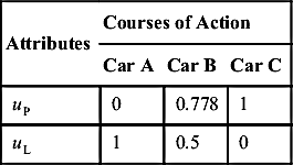
For example, a car buyer wants to buy a car with a long expected lifespan and a low price. The buyer narrowed down his or her choices to three alternatives: car A is a relatively expensive sedan with a reputation for longevity, car B is known for its reliability, and car C is a relatively inexpensive domestic automobile. The buyer has done some research and evaluated these three cars on both attributes, as shown in Table 2.8.
We set uP and uL for utilities of price and lifespan, respectively. Based on Table 2.8, we set uP(C) = uP($8000) = 1 for car C; uP(A) = uP($17,000) = 0 for car A. We assume the buyer is risk neutral on both price and lifespan; that is, r = 0 in the utility function defined in Eq. 2.14; that is, u(s) = s. Hence, uP(B) = uP($10,000) = 0.778 for car B. Similarly, we have uL(A) = uL(12) = 1; uL(C) = uL(6) = 0; hence, uL(B) = uL(9) = 0.5, as summarized in Table 2.9.
We assume that price is a lot more important factor than the lifespan of the car; therefore, we assign kP = 0.75 and kL = 0.25. Then, the utilities for the three alternatives are, respectively,
![]()
![]()
![]()
Example 2.1 offers more detailed illustration in the following section.
2.4.6.2. Multiplicative MAU functions
The other commonly employed MAU functions are multiplicative, which support preference interactions among attributes. A multiplicative MAU function is defined in Eq. 2.17:
 (2.17)
EXAMPLE 2.1
A different car buyer wants to buy a car with a long expected lifespan and a low price and has narrowed his or her choices down to the same three alternatives cars A, B, and C, with price and lifespan information listed in Table 2.8. The car buyer is risk averse in purchase price and is neutral in lifespan. We assume a utility function defined in Eq. 2.14 with r = 3, which characterizes the buyer's attitude toward risk. Calculate the combined utilities for the three alternatives using the additive form. We assume that price is equally as important as the lifespan of the car; therefore, kP = 0.5 and kL = 0.5.
Solutions
Because the buyer is risk neutral on lifespan, we have uL(A) = uL(12) = 1; uL(C) = uL(6) = 0; hence, uL(B) = uL(9) = 0.5. The buyer is risk averse with r = 3. From Eq. 2.15, we have
![]()
Hence, sP(B) = sP($10,000) = 0.778. Then, from the utility function defined in Eq. 2.14 with r = 3, we have
![]()
Then, the utilities for the three alternatives are, respectively,
![]()
![]()
![]()
![]() (2.18)
(2.18)
If the scaling factor is K = 0, indicating no interacting of attribute preference, this formulation is equivalent to its additive form, assuming the sum of all the scaling factors ki is 1; that is,  .
.
.It is shown in (Hyman 2003; Shtub et al. 1994) that if  , then −1 < K < 0, and if
  , then K > 0. Examples 2.2 and 2.3 provides a few more details on the multiplicative MAU function.
, then −1 < K < 0, and if , then K > 0. Examples 2.2 and 2.3 provides a few more details on the multiplicative MAU function.EXAMPLE 2.2
For m = 2 and k1 + k2 = 1, k1 > 0 and k2 > 0, show that the scaling factor defined in Eq. 2.18 is K = 0, and the multiplicative MAU function u defined in Eq. 2.17 becomes a linear MAU function.
Solutions
From Eq. 2.18, we have

Because k1 + k2 = 1, the above equation becomes 1 + K = 1 + K + K2k1k2. Because k1 > 0 and k2 > 0, we have K = 0. Hence,
EXAMPLE 2.3
Solutions
First, from Eq. 2.18, we have

Hence K = 2.
Then, the utilities for the three alternatives are, respectively,
![]()
![]()
![]()
..................Content has been hidden....................
You can't read the all page of ebook, please click here login for view all page.