3.6. Constrained Problems

Search in book...
Toggle Font Controls
Create new playlist

Name your new playlist

Playlist description (optional)
Sign In

Email address

Password

Forgot Password?

or

Continue with Facebook

Continue with Google
Sign Up

Full Name

Email address

Confirm Email Address

Password

or

Continue with Facebook

Continue with Google

3.6. Constrained Problems

The major difference between a constrained and unconstrained problem is that for a constrained problem, an optimal solution must be sought in a feasible region; for an unconstrained problem, the feasible region contains the entire design domain. For a constrained problem, bringing an infeasible design into a feasible region is critical, in which gradients of active constraints are taken into consideration when determining the search direction for the next design. In this section, we first outline the nature of the constrained optimization problem and the concept of solution techniques. In Section 3.6.2, we then discuss a widely accepted strategy for dealing with the constraint functions, the so-called ε-active strategy. Thereafter, in Sections 3.6.3–3.6.5 we discuss the mainstream solution techniques for solving constrained optimization problems, including SLP, SQP, and the feasible direction method. These solution techniques are capable of solving general optimization problems with multiple constraints and many design variables. Before closing out this section, we introduce the penalty method, which solves a constrained problem by converting it to an unconstrained problem, and then we solve the unconstrained problem using methods discussed in Section 3.5. For illustration purposes, we use simple examples of one or two design variables. Like Section 3.5, we offer sample MATLAB scripts (see Appendix A) for solving example problems.

3.6.1. Basic Concept

Recall the mathematical definition of the constrained optimization problem:

$Minimize: f (x)$ $Minimize: f (x)$

(3.67a)

$Subject to: g_{i} (x) \leq 0, i = 1, m$ $Subject to: g_{i} (x) \leq 0, i = 1, m$

(3.67b)

$h_{j} (x) = 0, j = 1, p$ $h_{j} (x) = 0, j = 1, p$

(3.67c)

$x_{k}^{ℓ} \leq x_{k} \leq x_{k}^{u}, k = 1, n$ $x_{k}^{ℓ} \leq x_{k} \leq x_{k}^{u}, k = 1, n$

(3.67d)

Similar to solving unconstrained optimization problems, all numerical methods are based on the iterative process, in which the next design point is updated by a search direction n and a step size α along the direction. The next design point x^k+1 is then obtained by evaluating the design at the current design point x^k (some methods include information from previous design iterations) as

$x^{k + 1} = x^{k} + Δ x^{k} = x^{k} + α^{k} n^{k}$ $x^{k + 1} = x^{k} + Δ x^{k} = x^{k} + α^{k} n^{k}$

(3.68)

For an unconstrained problem, the search direction n considers only the gradient of the objective function. For constrained problems, however, optimal solutions must be sought in the feasible region. Therefore, active constraints in addition to objective functions must be considered while determining the search direction as well as the step size. As with the unconstrained problems, all algorithms need an initial design to initiate the iterative process. The difference is for a constrained problem, the starting design can be feasible or infeasible, as illustrated in Figure 3.15a, in which a constrained optimization of two design variables x₁ and x₂ is assumed. The feasible region of the problem is identified on the surface of the objective function as well as projected onto the x₁–x₂ plane.

If an initial design is inside the feasible region, such as points A⁰ or B⁰, then we minimize the objective function by moving along its descent direction—say, the steepest descent direction—as if we are dealing with an unconstrained problem. We continue such iterations until either a minimum point is reached, such as the search path starting at point A⁰, or a constraint is encountered (i.e., the boundary of the feasible region is reached, like the path of initial design at point B⁰). Once the constraint boundary is encountered at point B¹, one strategy is to travel along a tangent line to the boundary, such as the direction B¹B² illustrated in Figure 3.15b. This leads to an infeasible point from where the constraints are corrected in order to again reach the feasible point B³. From there, the preceding steps are repeated until the optimum point is reached.

FIGURE 3.15 Concept illustration for solving a constrained optimization problem. (a) Paths illustrating different solution scenarios. (b) Top view of the feasible region, with a design point B residing on the boundary of the feasible region.

Another strategy is to deflect the tangential direction B¹B² toward the feasible region by a small angle θ when there are no equality constraints. Then, a line search is performed through the feasible region to reach the boundary point B⁴, as shown in Figure 3.15b. The procedure is then repeated from there.

When the starting point is infeasible, like points C⁰ or D⁰ in Figure 3.15a, one strategy is to correct constraint violations to reach the constraint boundary. From there, the strategies described in the preceding paragraph can be followed to reach the optimum point. For example, for D⁰, a similar path to that shown in path B¹B²B³ or B¹B⁴ in Figure 3.15b is followed. The case for point C⁰ is easier because the decent direction of objective function also corrects the constraint violations.

A good analogy for finding a minimum of a constrained problem is rolling a ball in a fenced downhill field. The boundary of the feasible region is the fence, and the surface of the downhill field is the objective function. When a ball is released at a location (i.e., the initial design), the ball rolls due to gravity. If the initial point is chosen such that the ball does not encounter the fence, the ball rolls to a local crest (minimum point). If an initial point chosen allows the ball to hit the fence, the ball rolls along the fence to reach a crest. If the initial point is outside the fenced area, the ball has to be thrown into the fenced area before it starts rolling.

Several algorithms based on the strategies described in the foregoing have been developed and evaluated. Some algorithms are better for a certain class of problems than others. In this section, we focus on general algorithms that have no restriction on the form of the objective or the constraint functions. Most of the algorithms that we will describe in this chapter can treat feasible and infeasible initial designs.

In general, numerical algorithms for solving constrained problems start with a linearization of the objective and constraint functions at the current design. The linearized subproblem is solved to determine the search direction n. Once the search direction is found, a line search is carried out to find an adequate step size α for the next design iteration. Following the general solution steps, we introduce three general methods: SLP, SQP, and the feasible direction method. Before we discuss the solution techniques, we discuss the ε-active strategy that determines the active constraints to incorporate for design optimization.

3.6.2. ε-Active Strategy

An ε-active constraint strategy (Arora 2012), shown in Figure 3.16, is often employed in solving constrained optimization problems. Inequality constraints in Eq. 3.67b and equality constraints of Eq. 3.67c are first normalized by their respective bounds:

$b_{i} = \frac{g_{i}}{g_{i}^{u}} - 1 \leq 0, i = 1, m$ $b_{i} = \frac{g_{i}}{g_{i}^{u}} - 1 \leq 0, i = 1, m$

(3.69a)

and

$e_{i} = \frac{h_{j}}{h_{j}^{u}} - 1, j = 1, p$ $e_{i} = \frac{h_{j}}{h_{j}^{u}} - 1, j = 1, p$

(3.69b)

Usually, when b_i (or e_i) is between two parameters CT (usually −0.03) and CTMIN (usually 0.005), g_i is active, as shown in Figure 3.16. When b_i is less than CT, the constraint function is inactive or feasible. When b_i is larger than CTMIN, the constraint function is violated. Note that CTMIN-CT = ε.

3.6.3. The Sequential Linear Programming Algorithm

The original optimization problem stated in Eq. 3.67 is first linearized by writing Taylor's expansions for the objective and constraint functions at the current design x^k as below.

Minimize the linearized objective function:

$f (x^{k + 1}) = f (x^{k} + Δ x^{k}) \approx f (x^{k}) + \nabla f^{T} (x^{k}) Δ x^{k}$ $f (x^{k + 1}) = f (x^{k} + Δ x^{k}) \approx f (x^{k}) + \nabla f^{T} (x^{k}) Δ x^{k}$

(3.70a)

subject to the linearized inequality constraints

$g_{i} (x^{k + 1}) = g_{i} (x^{k} + Δ x^{k}) \approx g_{i} (x^{k}) + \nabla g_{i}^{T} (x^{k}) Δ x^{k} \leq 0; i = 1, m$ $g_{i} (x^{k + 1}) = g_{i} (x^{k} + Δ x^{k}) \approx g_{i} (x^{k}) + \nabla g_{i}^{T} (x^{k}) Δ x^{k} \leq 0; i = 1, m$

(3.70b)

and the linearized equality constraints

FIGURE 3.16 ε-Active constraint strategy.

$h_{j} (x^{k + 1}) = h_{j} (x^{k} + Δ x^{k}) \approx h_{j} (x^{k}) + \nabla h_{j}^{T} (x^{k}) Δ x^{k} = 0; j = 1, p$ $h_{j} (x^{k + 1}) = h_{j} (x^{k} + Δ x^{k}) \approx h_{j} (x^{k}) + \nabla h_{j}^{T} (x^{k}) Δ x^{k} = 0; j = 1, p$

(3.70c)

in which ∇f(Δx^k), ∇g_i(Δx^k), and ∇h_j(Δx^k) are the gradients of the objective function, the ith inequality constraint and the jth equality constraint, respectively, and ≈ implies approximate equality.

To simplify the mathematical notations in our discussion, we rewrite the linearized equations in Eq. 3.70 as

$Minimize: \bar{f} = c^{T} d$ $Minimize: \bar{f} = c^{T} d$

(3.71a)

$Subject to: A^{T} d \leq b$ $Subject to: A^{T} d \leq b$

(3.71b)

$N^{T} d = e$ $N^{T} d = e$

(3.71c)

$- Δ_{ℓ} \leq d \leq Δ_{u}$ $- Δ_{ℓ} \leq d \leq Δ_{u}$

(3.71d)

where

$c_{n \times 1} = \nabla f (x^{k}) = {[\partial f (x^{k}) / \partial x_{1}, \partial f (x^{k}) / \partial x_{2}, \dots, \partial f (x^{k}) / \partial x_{n}]}^{T};$ $c_{n \times 1} = \nabla f (x^{k}) = {[\partial f (x^{k}) / \partial x_{1}, \partial f (x^{k}) / \partial x_{2}, \dots, \partial f (x^{k}) / \partial x_{n}]}^{T};$

$d_{n \times 1} = Δ x^{k} = {[Δ x_{1}^{k}, Δ x_{2}^{k}, \dots, Δ x_{n}^{k}]}^{T};$ $d_{n \times 1} = Δ x^{k} = {[Δ x_{1}^{k}, Δ x_{2}^{k}, \dots, Δ x_{n}^{k}]}^{T};$

$A_{m \times n} = {[\nabla g_{1} (x^{k}), \nabla g_{2} (x^{k}), \dots, \nabla g_{m} (x^{k})]}_{m \times n},$ $A_{m \times n} = {[\nabla g_{1} (x^{k}), \nabla g_{2} (x^{k}), \dots, \nabla g_{m} (x^{k})]}_{m \times n},$

$in which \nabla g_{i} (x^{k}) = {[\partial g_{i} (x^{k}) / \partial x_{1}, \partial g_{i} (x^{k}) / \partial x_{2}, \dots, \partial g_{i} (x^{k}) / \partial x_{n}]}_{n \times 1}^{T};$ $in which \nabla g_{i} (x^{k}) = {[\partial g_{i} (x^{k}) / \partial x_{1}, \partial g_{i} (x^{k}) / \partial x_{2}, \dots, \partial g_{i} (x^{k}) / \partial x_{n}]}_{n \times 1}^{T};$

$N_{p \times n} = {[\nabla h_{1} (x^{k}), \nabla h_{2} (x^{k}), \dots, \nabla h_{p} (x^{k})]}_{p \times n},$ $N_{p \times n} = {[\nabla h_{1} (x^{k}), \nabla h_{2} (x^{k}), \dots, \nabla h_{p} (x^{k})]}_{p \times n},$

$in which \nabla h_{i} (x^{k}) = {[\partial h_{i} (x^{k}) / \partial x_{1}, \partial h_{i} (x^{k}) / \partial x_{2}, \dots, \partial h_{i} (x^{k}) / \partial x_{n}]}_{n \times 1}^{T};$ $in which \nabla h_{i} (x^{k}) = {[\partial h_{i} (x^{k}) / \partial x_{1}, \partial h_{i} (x^{k}) / \partial x_{2}, \dots, \partial h_{i} (x^{k}) / \partial x_{n}]}_{n \times 1}^{T};$

$b_{m \times 1} = - g_{i} (x^{k}) = {[- g_{1} (x^{k}), - g_{2} (x^{k}), \dots, - g_{m} (x^{k})]}_{m \times 1};$ $b_{m \times 1} = - g_{i} (x^{k}) = {[- g_{1} (x^{k}), - g_{2} (x^{k}), \dots, - g_{m} (x^{k})]}_{m \times 1};$

and

$e_{m \times 1} = - h_{i} (x^{k}) = {[- h_{1} (x^{k}), - h_{2} (x^{k}), \dots, - h_{p} (x^{k})]}_{p \times 1} .$ $e_{m \times 1} = - h_{i} (x^{k}) = {[- h_{1} (x^{k}), - h_{2} (x^{k}), \dots, - h_{p} (x^{k})]}_{p \times 1} .$

Note that in Eq. 3.71a, f(x^k) is dropped.

Δ_{ℓ} = {[Δ_{1 ℓ}^{k}, Δ_{2 ℓ}^{k}, \dots, Δ_{n ℓ}^{k}]}_{n \times 1}^{T}

$Δ_{ℓ} = {[Δ_{1 ℓ}^{k}, Δ_{2 ℓ}^{k}, \dots, Δ_{n ℓ}^{k}]}_{n \times 1}^{T}$

and

Δ_{u} = {[Δ_{1 u}^{k}, Δ_{2 u}^{k}, \dots, Δ_{n u}^{k}]}_{n \times 1}^{T}

$Δ_{u} = {[Δ_{1 u}^{k}, Δ_{2 u}^{k}, \dots, Δ_{n u}^{k}]}_{n \times 1}^{T}$

are the move limits—that is, the maximum allowed decrease and increase in the design variables at the kth design iteration. Note that the move limits make the linearized subproblem bounded and give the design changes directly without performing the line search for a step size α. Therefore, no line search is required in SLP. Choosing adequate move limits is critical to the SLP. More about the move limits will be discussed in Example 3.16.

As discussed before, the SLP algorithm starts with an initial design x⁰. At the kth design iteration, we evaluate the objective and constraint functions as well as their gradients at the current design x^k. We select move limits Δ_iℓ^k and Δ_iu^k to define an LP subproblem of Eq. 3.71. Solve the linearized subproblem for d^k, and update the design for the next iteration as x^k+1 = x^k + d^k. The process repeats until convergent criteria are met. In general, the convergent criteria for an LP subproblem include

$g_{i} (x^{k + 1}) \leq ε_{1}, i = 1, m; | h_{j} (x^{k + 1}) | \leq ε_{1}, j = 1, p; and ‖ d^{k} ‖ \leq ε_{2}$ $g_{i} (x^{k + 1}) \leq ε_{1}, i = 1, m; | h_{j} (x^{k + 1}) | \leq ε_{1}, j = 1, p; and ‖ d^{k} ‖ \leq ε_{2}$

(3.72)

EXAMPLE 3.16

Solve Example 3.7 with one additional equality constraint using SLP. The optimization problem is restated as below.

$Minimize: f (x) = {(x_{1} - 3)}^{2} + {(x_{2} - 3)}^{2}$ $Minimize: f (x) = {(x_{1} - 3)}^{2} + {(x_{2} - 3)}^{2}$

(3.73a)

$Subject to: g_{1} (x) = 3 x_{1} + x_{2} - 6 \leq 0$ $Subject to: g_{1} (x) = 3 x_{1} + x_{2} - 6 \leq 0$

(3.73b)

$h_{1} (x) = x_{1} - x_{2} = 0$ $h_{1} (x) = x_{1} - x_{2} = 0$

(3.73c)

$0 \leq x_{1}, 0 \leq x_{2}$ $0 \leq x_{1}, 0 \leq x_{2}$

(3.73d)

Solutions

We sketch the feasible region bounded by inequality constraint g₁(x) ≤ 0, side constraints, and equality constraint h₁(x) = 0, as shown below. As is obvious in the sketch, the optimal solution is found at x^∗ = (1.5, 1.5), the intersection of g₁(x) = 0, and h₁(x) = 0, in which f(x) = 4.5.

Now we use this example to illustrate the solution steps using SLP. We assume an initial design at x⁰ = (2, 2). At the initial design, we have f(2, 2) = (x₁−3)² + (x₂−3)² = 2, g₁(2, 2) = 3x₁ + x₂ − 6 = 2 > 0, and h₁(2, 2) = 0. The inequality constraint g₁ is greater than 0; therefore, this constraint is violated. The initial design is not in the feasible region, as also illustrated in the figure above. The optimization problem defined in Eqs 3.73a–3.73d is linearized as follows:

$Minimize: \bar{f} = c^{T} d = [\begin{matrix} 2 (x_{1} - 3) & 2 (x_{2} - 3) \end{matrix}] [\begin{matrix} Δ x_{1} \\ Δ x_{2} \end{matrix}]$ $Minimize: \bar{f} = c^{T} d = [\begin{matrix} 2 (x_{1} - 3) & 2 (x_{2} - 3) \end{matrix}] [\begin{matrix} Δ x_{1} \\ Δ x_{2} \end{matrix}]$

(3.73e)

$Subject to: A^{T} d \leq b; i .e ., [\begin{matrix} 3 & 1 \end{matrix}] [\begin{matrix} Δ x_{1} \\ Δ x_{2} \end{matrix}] \leq 6, or {\bar{g}}_{1} = 3 Δ x_{1} + Δ x_{2} - 6 \leq 0$ $Subject to: A^{T} d \leq b; i .e ., [\begin{matrix} 3 & 1 \end{matrix}] [\begin{matrix} Δ x_{1} \\ Δ x_{2} \end{matrix}] \leq 6, or {\bar{g}}_{1} = 3 Δ x_{1} + Δ x_{2} - 6 \leq 0$

(3.73f)

$N^{T} d = e; i .e ., [\begin{matrix} 1 & - 1 \end{matrix}] [\begin{matrix} Δ x_{1} \\ Δ x_{2} \end{matrix}] = 0, or {\bar{h}}_{1} = Δ x_{1} - Δ x_{2} = 0$ $N^{T} d = e; i .e ., [\begin{matrix} 1 & - 1 \end{matrix}] [\begin{matrix} Δ x_{1} \\ Δ x_{2} \end{matrix}] = 0, or {\bar{h}}_{1} = Δ x_{1} - Δ x_{2} = 0$

(3.73g)

$- 0.2 \leq Δ x_{1} \leq 0.2, - 0.2 \leq Δ x_{2} \leq 0.2$ $- 0.2 \leq Δ x_{1} \leq 0.2, - 0.2 \leq Δ x_{2} \leq 0.2$

(3.73h)

We have chosen the move limits to be 0.2, which is 10% of the current design variable values, as shown in Eq. 3.73h. At the initial design, x⁰ = (2, 2), we are minimizing

\bar{f} = [\begin{matrix} - 2 & - 2 \end{matrix}] [\begin{matrix} Δ x_{1} \\ Δ x_{2} \end{matrix}] = - 2 Δ x_{1} - 2 Δ x_{2}

$\bar{f} = [\begin{matrix} - 2 & - 2 \end{matrix}] [\begin{matrix} Δ x_{1} \\ Δ x_{2} \end{matrix}] = - 2 Δ x_{1} - 2 Δ x_{2}$

subject to constraints (Eqs 3.73f–3.73h). The subproblem has two variables; it can be solved by referring to the sketch below. Because we chose 0.2 as the move limits, the solution to the LP subproblem must lie in the region of the small dotted square box shown below. It can be seen that there is no feasible solution to this linearized subproblem because the small box does not intersect the line

{\bar{g}}_{1} = 0

${\bar{g}}_{1} = 0$

. We must enlarge this region by increasing the move limits. Thus, we note that if the move limits are too restrictive, the linearized subproblem may not have a solution.

If we choose the move limits to be 1—that is, 50% of the design variable values—then the design must lie within a larger box ABCD of 2×2 as shown above. Hence the feasible region of the LP problem is now the triangle AED intersecting

{\bar{h}}_{1}

${\bar{h}}_{1}$

= 0 (that is, line segment AF). Therefore, the optimal solution of the LP problem is found at point F: x_F = (1.5, 1.5), where

\bar{f}

$\bar{f}$

= −6. That is, d = [Δx₁⁰, Δx₂⁰]^T = [−0.5, −0.5]^T, and x¹ = x⁰ + d = [2, 2]^T + [−0.5, −0.5]^T = [1.5, 1.5]^T = x_F.

In the next design x¹, we evaluate the objective and constraint functions of the original optimization problem as well as their gradients. We have f(1.5, 1.5) = (x₁−3)² + (x₂−3)² = 4.5, g₁(1.5, 1.5) = 3x₁ + x₂ − 6 = 0, and h₁(1.5, 1.5) = 0. The design is feasible. Again, at the design iteration x¹ = (1.5, 1.5), we create the LP problem as

$Minimizing : \bar{f} = [\begin{matrix} - 3 & - 3 \end{matrix}] [\begin{matrix} Δ x_{1} \\ Δ x_{2} \end{matrix}] = - 3 Δ x_{1} - 3 Δ x_{2}$ $Minimizing : \bar{f} = [\begin{matrix} - 3 & - 3 \end{matrix}] [\begin{matrix} Δ x_{1} \\ Δ x_{2} \end{matrix}] = - 3 Δ x_{1} - 3 Δ x_{2}$

$Subject to : {\bar{g}}_{1} = 3 Δ x_{1} + Δ x_{2} - 6 \leq 0$ $Subject to : {\bar{g}}_{1} = 3 Δ x_{1} + Δ x_{2} - 6 \leq 0$

${\bar{h}}_{1} = Δ x_{1} - Δ x_{2} = 0$ ${\bar{h}}_{1} = Δ x_{1} - Δ x_{2} = 0$

$- 1 \leq Δ x_{1} \leq 1, - 1 Δ x_{2} \leq 1$ $- 1 \leq Δ x_{1} \leq 1, - 1 Δ x_{2} \leq 1$

As illustrated in the figure next page, the feasible region of the LP subproblem is now the polygon A₁E₁F₁D₁ intersecting

{\bar{h}}_{1}

${\bar{h}}_{1}$

= 0. Therefore, the optimal solution of the LP problem is found again at x¹ = (1.5, 1.5), the same point. That is, in this design iteration, d = [Δx₁¹, Δx₂¹]^T = [0, 0]^T.

At this point, the convergent criterion stated in Eq. 3.72, for example, ||d¹|| = 0 ≤ ε₂, is satisfied; hence, an optimal solution is found at x¹ = (1.5, 1.5).

In fact, for this particular problem, it takes only one iteration to find the optimal solution. In general, this may not be the case. An iterative process often takes numerous iterations to achieve a convergent solution.

Although the SLP algorithm is a simple and straightforward approach to solving constrained optimization problems, it should not be used as a black-box approach for engineering design problems. The selection of move limits is in essence trial and error and can be best achieved in an interactive mode. Also, the method may not converge to the precise minimum because no descent function is defined, and the line search is not performed along the search direction to compute a step size. Nevertheless, this method may be used to obtain improved designs in practice. It is a good method to include in our toolbox for solving constrained optimization problems.

3.6.4. The Sequential Quadratic Programming Algorithm

The SQP algorithm incorporates second-order information about the problem functions in determining a search direction n and step size α. A search direction in the design space is calculated by utilizing the values and the gradients of the objective and constraint functions. A quadratic programming subproblem is defined as

$Minimize: \bar{f} = c^{T} d + \frac{1}{2} d^{T} d$ $Minimize: \bar{f} = c^{T} d + \frac{1}{2} d^{T} d$

(3.74a)

$Subject to: A^{T} d \leq b$ $Subject to: A^{T} d \leq b$

(3.74b)

$N^{T} d = e$ $N^{T} d = e$

(3.74c)

in which a quadratic term is added to the objective function

\bar{f}

$\bar{f}$

and the constraint functions (3.74b) and (3.74c) are identical to those of LP subproblem, except that there is no need to define the move limits. The solution of the QP problem d defines the search direction n (where n = d/||d||). Once the search direction is determined, a line search is carried out to find an adequate step size α. The process repeats until the convergent criteria defined in Eq. 3.72 are met.

EXAMPLE 3.17

Solve the same problem of Example 3.16 using SQP.

Solutions

We assume the same initial design at x⁰ = (2, 2). At the initial design, we have f(2, 2) = (x₁−3)² + (x₂−3)² = 2, g₁(2, 2) = 3x₁ + x₂ − 6 = 2 > 0, and h₁(2, 2) = 0. The initial design is infeasible. The QP subproblem can be written as

$Minimize: \bar{f} = c^{T} d + \frac{1}{2} d^{T} d = [\begin{matrix} 2 (x_{1} - 3) & 2 (x_{2} - 3) \end{matrix}] [\begin{matrix} Δ x_{1} \\ Δ x_{2} \end{matrix}] + \frac{1}{2} [\begin{matrix} Δ x_{1} & Δ x_{2} \end{matrix}] [\begin{matrix} Δ x_{1} \\ Δ x_{2} \end{matrix}]$ $Minimize: \bar{f} = c^{T} d + \frac{1}{2} d^{T} d = [\begin{matrix} 2 (x_{1} - 3) & 2 (x_{2} - 3) \end{matrix}] [\begin{matrix} Δ x_{1} \\ Δ x_{2} \end{matrix}] + \frac{1}{2} [\begin{matrix} Δ x_{1} & Δ x_{2} \end{matrix}] [\begin{matrix} Δ x_{1} \\ Δ x_{2} \end{matrix}]$

(3.75a)

$Subject to: {\bar{g}}_{1} = 3 Δ x_{1} + Δ x_{2} - 6 \leq 0$ $Subject to: {\bar{g}}_{1} = 3 Δ x_{1} + Δ x_{2} - 6 \leq 0$

(3.75b)

${\bar{h}}_{1} = Δ x_{1} - Δ x_{2} = 0$ ${\bar{h}}_{1} = Δ x_{1} - Δ x_{2} = 0$

(3.75c)

At the initial design, x⁰ = (2, 2), we are minimizing

$\bar{f} = [\begin{matrix} - 2 & - 2 \end{matrix}] [\begin{matrix} Δ x_{1} \\ Δ x_{2} \end{matrix}] + \frac{1}{2} [\begin{matrix} Δ x_{1} & Δ x_{2} \end{matrix}] [\begin{matrix} Δ x_{1} \\ Δ x_{2} \end{matrix}] = - 2 Δ x_{1} - 2 Δ x_{2} + \frac{1}{2} (Δ x_{1}^{2} + Δ x_{2}^{2})$ $\bar{f} = [\begin{matrix} - 2 & - 2 \end{matrix}] [\begin{matrix} Δ x_{1} \\ Δ x_{2} \end{matrix}] + \frac{1}{2} [\begin{matrix} Δ x_{1} & Δ x_{2} \end{matrix}] [\begin{matrix} Δ x_{1} \\ Δ x_{2} \end{matrix}] = - 2 Δ x_{1} - 2 Δ x_{2} + \frac{1}{2} (Δ x_{1}^{2} + Δ x_{2}^{2})$

subject to constraint Eqs 3.75b and 3.75c. The QP subproblem can be solved by either using the KKT condition or graphical method. We use the graphical method for this example.

Referring to the sketch below, the optimal solution to the QP subproblem is found at point F: x_F = (1.5, 1.5), where

\bar{f} = - 3.75

$\bar{f} = - 3.75$

. That is,

d = {[Δ x_{1}^{0}, Δ x_{2}^{0}]}^{T} = {[- 0.5, - 0.5]}^{T} .

$d = {[Δ x_{1}^{0}, Δ x_{2}^{0}]}^{T} = {[- 0.5, - 0.5]}^{T} .$

Note that the quadratic function

\bar{f}

$\bar{f}$

is sketched using the MATLAB script shown in Appendix A (Script 12).

For the next iteration, we have

n = d / ‖ d ‖ = {[- 0.707, - 0.707]}^{T}

$n = d / ‖ d ‖ = {[- 0.707, - 0.707]}^{T}$

and assume a step size α = 1. Hence, for the next design, x¹ = x⁰ + αn⁰ = [2, 2]^T + 1[−0.707, −0.707]^T = [1.293, 1.293]^T.

In the next design x¹, we evaluate the objective and constraint functions of the original optimization problem as well as their gradients. We have f(1.293, 1.293) = (x₁ − 3)² + (x₂ − 3)² = 5.828, g₁(1.293, 1.293) = 3x₁ + x₂ − 6 = −0.828, and h₁(1.293, 1.293) = 0. The design is feasible. Again, at the design iteration x¹ = (1.293, 1.293), we create the QP problem as

$Minimizing : \bar{f} = [\begin{matrix} - 3.414 - 3.414 \end{matrix}] [\begin{matrix} Δ x_{1} \\ Δ x_{2} \end{matrix}] + \frac{1}{2} [\begin{matrix} Δ x_{1} Δ x_{2} \end{matrix}] [\begin{matrix} Δ x_{1} \\ Δ x_{2} \end{matrix}] = - 3.414 Δ x_{1} - 3.414 Δ x_{2} + \frac{1}{2} (Δ x_{1}^{2} + Δ x_{2}^{2})$ $Minimizing : \bar{f} = [\begin{matrix} - 3.414 - 3.414 \end{matrix}] [\begin{matrix} Δ x_{1} \\ Δ x_{2} \end{matrix}] + \frac{1}{2} [\begin{matrix} Δ x_{1} Δ x_{2} \end{matrix}] [\begin{matrix} Δ x_{1} \\ Δ x_{2} \end{matrix}] = - 3.414 Δ x_{1} - 3.414 Δ x_{2} + \frac{1}{2} (Δ x_{1}^{2} + Δ x_{2}^{2})$

$Subject to : {\bar{g}}_{1} = 3 Δ x_{1} + Δ x_{2} - 6 \leq 0$ $Subject to : {\bar{g}}_{1} = 3 Δ x_{1} + Δ x_{2} - 6 \leq 0$

${\bar{h}}_{1} = Δ x_{1} - Δ x_{2} = 0$ ${\bar{h}}_{1} = Δ x_{1} - Δ x_{2} = 0$

The optimal design of the QP problem is found again at x¹ = (1.5, 1.5), the same point since the constraint functions are unchanged. That is,

d = {[Δ x_{1}^{1}, Δ x_{2}^{1}]}^{T} = {[0.207, 0.207]}^{T}

$d = {[Δ x_{1}^{1}, Δ x_{2}^{1}]}^{T} = {[0.207, 0.207]}^{T}$

. The process continues until the convergent criterion stated in Eq. 3.72 are satisfied. After several iteration, an optimal solution is found at x^∗ = (1.5, 1.5).

3.6.5. Feasible Direction Method

The basic idea of the feasible direction method is to determine a search direction that moves from the current design point to an improved feasible point in the design space. Thus, given a design x^k, an improving feasible search direction n^k is determined such that for a sufficiently small step size α > 0, the new design, x^k+1 = x^k + α^kn^k is feasible, and the new objective function is smaller than the current one; that is, f(x^k+1) < f(x^k). Note that n is a normalized vector, defined as n = d/||d||, where d is the nonnormalized search direction solved from a subproblem to be discussed.

Because along the search direction d^k the objective function must decrease without violating the applied constraints, taking in account only inequality constraints, it must result that

$\nabla f (x^{k}) \cdot d^{k} < 0$ $\nabla f (x^{k}) \cdot d^{k} < 0$

(3.76)

and

$\nabla g_{i} (x^{k}) \cdot d^{k} < 0, for i \in I_{k}$ $\nabla g_{i} (x^{k}) \cdot d^{k} < 0, for i \in I_{k}$

(3.77)

I_k is the potential constraint set at the current point, defined as

$I_{k} \equiv {i | g_{i} {(x)}^{k} + ε \geq 0 i = 1, m}$ $I_{k} \equiv {i | g_{i} {(x)}^{k} + ε \geq 0 i = 1, m}$

(3.78)

Note that ε is a small positive number, selected to determine ε-active constraints as discussed in Section 3.6.1. Note that g_i(x) is normalized as in Eq. 3.69a. The inequality constraints enclosed in the set of Eq. 3.78 are either violated or ε-active, meaning they have to be considered in determining a search direction that brings the design into the feasible region. Equations 3.76 and 3.77 are referred to as usability and feasibility requirements, respectively. A geometrical interpretation of the requirements is shown in Figure 3.17 for a two-variable optimization problem, in which the search direction n points to the usable-feasible region.

This method has been developed and applied mostly to optimization problems with inequality constraints. This is because, in implementation, the search direction n is determined by defining a linearized subproblem (to be discussed next) at the current feasible point, and the step size α is determined to reduce the objective function as well as maintain feasibility of design. Because linear approximations are used, it is difficult to maintain feasibility with respect to the equality constraints. Although some procedures have been developed to treat equality constraints in these methods, we will describe the method for problems with only inequality constraints.

FIGURE 3.17 Geometric description of the feasible direction method.

The desired search direction d will meet the requirements of usability and feasibility, and it gives the highest reduction of the objective function along it. Mathematically, it is obtained by solving the following linear subproblem in d:

$Minimize : β$ $Minimize : β$

(3.79a)

$Subject to: \nabla f^{T} (x) d - β \leq 0$ $Subject to: \nabla f^{T} (x) d - β \leq 0$

(3.79b)

$\nabla g_{i}^{T} (x) d - β \leq 0, for i \in I_{k}$ $\nabla g_{i}^{T} (x) d - β \leq 0, for i \in I_{k}$

(3.79c)

$d_{j}^{ℓ} \leq d_{j} \leq d_{j}^{u}, for j = 1, n$ $d_{j}^{ℓ} \leq d_{j} \leq d_{j}^{u}, for j = 1, n$

(3.79d)

Note that this is a linear programming problem. If β < 0, then d is an improving feasible direction. If β = 0, then the current design satisfies the KKT necessary conditions and the optimization process is terminated. To compute the improved design in this direction, a step size α is needed.

EXAMPLE 3.18

Solve the optimization problem of Example 3.7 using the feasible direction method. The problem is restated below:

$Minimize: f (x) = {(x_{1} - 3)}^{2} + {(x_{2} - 3)}^{2}$ $Minimize: f (x) = {(x_{1} - 3)}^{2} + {(x_{2} - 3)}^{2}$

(3.80a)

$Subject to: g_{1} (x) = 3 x_{1} + x_{2} - 6 \leq 0$ $Subject to: g_{1} (x) = 3 x_{1} + x_{2} - 6 \leq 0$

(3.80b)

$0 \leq x_{1}, and 0 \leq x_{2}$ $0 \leq x_{1}, and 0 \leq x_{2}$

(3.80c)

Solutions

Referring to the sketch of Example 3.7, the optimal solution is found as x^∗ = (1.2, 2.4), in which f(x) = 3.6. In this example, we present two cases of two respective initial designs, one in the feasible region and the other one in the infeasible region.

Case A: feasible initial design at x⁰ = (1, 1). From Eq. 3.79, a subproblem can be written at the initial design as

$Minimize : β$ $Minimize : β$

(3.80d)

$Subject to: q_{1} = - 4 d_{1} - 4 d_{2} - β \leq 0$ $Subject to: q_{1} = - 4 d_{1} - 4 d_{2} - β \leq 0$

(3.80e)

$- 1 \leq d_{1} \leq 1, - 1 \leq d_{2} \leq 1$ $- 1 \leq d_{1} \leq 1, - 1 \leq d_{2} \leq 1$

(3.80f)

Note that we do not need to include the linearized constraint equation g₁ ≤ 0 because the design is feasible. We assume lower and upper bounds of the subproblem as −1 and 1, respectively, as stated in Eq. 3.80f.

We sketch the feasible region defined by Eqs 3.80e and 3.80f with β = 0 and −8, respectively, as shown below. For β = 0, the feasible region is the triangle ABC, and for β = −8, the feasible region reduces to a single point C = (1, 1). As is obvious in the sketches below, the optimal solution of the subproblem is found at C = (1, 1), in which β = −8.

Certainly, if the bounds of d₁ and d₂ are changed, the solution changes as well. However, the search direction defined by n = d/||d|| = [1, 1]^T/||[1, 1]^T|| = [0.707, 0. 707]^T remains the same. From Eq. 3.79b, we have

$\nabla f^{T} (1,1) d = [- 4, - 4] {[1,1]}^{T} = - 8 (= β) < 0$ $\nabla f^{T} (1,1) d = [- 4, - 4] {[1,1]}^{T} = - 8 (= β) < 0$

Note that ∇f^T d is a dot product of ∇f^T and d. Geometrically, (∇f^T d)/||∇f^T d|| = −1 is the angle between the vectors ∇f^T and d—in this case 180°, as shown below. This is because the initial design is feasible, and the search direction n (or d) is the negative of the gradient of the objective function ∇f.

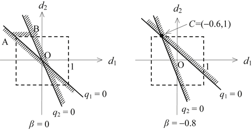
Case B: infeasible initial design at x⁰ = (2, 2). From Eq. 3.79, a subproblem can be written at the initial design as

$Minimize : β$ $Minimize : β$

(3.80g)

$Subject to: q_{1} = - 2 d_{1} - 2 d_{2} - β \leq 0$ $Subject to: q_{1} = - 2 d_{1} - 2 d_{2} - β \leq 0$

(3.80h)

$q_{2} = 3 d_{1} + d_{2} - β \leq 0$ $q_{2} = 3 d_{1} + d_{2} - β \leq 0$

(3.80i)

$- 1 \leq d_{1} \leq 1, - 1 \leq d_{2} \leq 1$ $- 1 \leq d_{1} \leq 1, - 1 \leq d_{2} \leq 1$

(3.80j)

Similar to Case A, we sketch the feasible region defined by of Eqs 3.80h–3.80j with β = 0 and −0.8, respectively, as shown below. For β = 0, the feasible region is the triangle ABO, and for β = −0.8, the feasible region reduces to a single point at C = (−0.6, 1). As is obvious in the sketches, the optimal solution of the subproblem is found at C = (−0.6, 1), in which β = −0.8.

The search direction is found as

n = d / ‖ d ‖ = {{[- 0.6, 1]}^{T} / ‖ [- 0.6, 1] ‖}^{T} = {[- 0.441, 0.735]}^{T}

$n = d / ‖ d ‖ = {{[- 0.6, 1]}^{T} / ‖ [- 0.6, 1] ‖}^{T} = {[- 0.441, 0.735]}^{T}$

. From Eqs 3.79b and 3.79c, we have

$\nabla f^{T} (2,2) d = [- 2, - 2] {[- 0.6, 1]}^{T} = - 0.8 (= β) < 0, and \nabla g_{i}^{T} (2,2) d = [3,1] {[- 0.6, 1]}^{T} = - 0.8 < 0$ $\nabla f^{T} (2,2) d = [- 2, - 2] {[- 0.6, 1]}^{T} = - 0.8 (= β) < 0, and \nabla g_{i}^{T} (2,2) d = [3,1] {[- 0.6, 1]}^{T} = - 0.8 < 0$

Geometrically, they are the respective angles between the vectors ∇f ^T and d and ∇g_i^T and d, as shown below. Because the design is infeasible, the gradient of the active constraint is taken into consideration in calculating the search direction. In fact, because the same parameter β is employed in the constraint equations of the subproblem, the search direction n points in a direction that splits the angle between −∇f and −∇g₁.

In the constraint equations of the subproblem stated in Eqs 3.79b and 3.79c, the same parameter β is employed. As demonstrated in Case B of Example 3.18, the same β leads to a search direction n pointing in a direction that splits the angle between −∇f and −∇g₁, in which g₁ is an active constraint function.

To determine a better feasible direction d, the constraints of Eq. 3.79c can be modified as

$\nabla g_{i}^{T} (x) d - θ_{i} β \leq 0, for i \in I_{K}$ $\nabla g_{i}^{T} (x) d - θ_{i} β \leq 0, for i \in I_{K}$

(3.81)

where θ_i is called the push-off factor. The greater the value of θ_i, the more the direction vector d is pushed into the feasible region. The reason for introducing θ_i is to prevent the iterations from repeatedly hitting the constraint boundary and slowing down the convergence.

EXAMPLE 3.19

Find the search directions n for Case B of Example 3.18, assuming θ₁ = 0, 0.5, and 1.5.

Solutions

We show the solutions in the following four cases.

Case A: θ₁ = 0. From Eqs 3.79 and 3.81, a subproblem can be written at the initial design as

$Minimize : β$ $Minimize : β$

(3.82a)

$Subject to: q_{1} = - 2 d_{1} - 2 d_{2} - β \leq 0$ $Subject to: q_{1} = - 2 d_{1} - 2 d_{2} - β \leq 0$

(3.82b)

$q_{2} = 3 d_{1} + d_{2} \leq 0$ $q_{2} = 3 d_{1} + d_{2} \leq 0$

(3.82c)

$- 1 \leq d_{1} \leq 1, - 1 \leq d_{2} \leq 1$ $- 1 \leq d_{1} \leq 1, - 1 \leq d_{2} \leq 1$

(3.82d)

Following the similar approach as in Example 3.18, the solution to the subproblem defined in Eqs 3.82a–3.82d is found at d = (−1/3, 1) with β = −4/3. In fact, the search direction points in a direction that is parallel to the active constraint g₁ at the current design x⁰; i.e., the search direction is perpendicular to the gradient of the constraint function ∇g₁, as shown below in the vector d(0).

Case B: θ₁ = 0.5. The constraint equation q₂ of the subproblem becomes

$q_{2} = 3 d_{1} + d_{2} - 0.5 β \leq 0$ $q_{2} = 3 d_{1} + d_{2} - 0.5 β \leq 0$

(3.82e)

The solution to the subproblem is found at d = (−1/2, 1) with β = −1. The search direction n leans to −∇g₁, as shown in the figure above in the vector d(0.5). That is, the design is pushed more into the feasible region compared to the case where θ₁ = 0.

Case C: θ₁ = 1. The constraint equation q₂ of the subproblem becomes

$q_{2} = 3 d_{1} + d_{2} - β \leq 0$ $q_{2} = 3 d_{1} + d_{2} - β \leq 0$

(3.82f)

The solution to the subproblem is found at d = (−0.6, 1) with β = −0.8. The search direction d leans more to −∇g₁, as shown in the figure above in the vector d(1).

Case D: θ₁ = 1.5. The constraint equation q₂ of the subproblem becomes

$q_{2} = 3 d_{1} + d_{2} - 1.5 β \leq 0$ $q_{2} = 3 d_{1} + d_{2} - 1.5 β \leq 0$

(3.82g)

The solution to the subproblem is found at d = (−2/3, 1) with β = −2/3. The search direction d leans more to −∇g₁, as shown in the figure above in the vector d(1.5).

3.6.6. Penalty Method

A penalty method replaces a constrained optimization problem by a series of unconstrained problems whose solutions ideally converge to the solution of the original constrained problem. The unconstrained problems are formed by adding a term, called a penalty function, to the objective function that consists of a penalty parameter multiplied by a measure of violation of the constraints. The measure of violation is nonzero when the constraints are violated and is zero in the region where constraints are not violated.

Recall that a constrained optimization problem considered is defined as

$\underset{x \in S}{Minimize} f (x)$ $\underset{x \in S}{Minimize} f (x)$

(3.83)

where S is the set of feasible designs defined by equality and inequality constraints. Using the penalty method, Eq. 3.83 is first converted to an unconstrained problem as

$Minimize Φ (x, r_{p}) = f (x) + r_{p} p (x)$ $Minimize Φ (x, r_{p}) = f (x) + r_{p} p (x)$

(3.84)

where f(x) is the original objective function, p(x) is an imposed penalty function, and r_p is a multiplier that determines the magnitude of the penalty. The function Ф(x, r_p) is called pseudo-objective function.

There are numerous ways to create a penalty function. One of the easiest is called exterior penalty (Vanderplaats 2007), in which a penalty function is defined as

$p (x) = \sum_{i = 1}^{m} {max [0, g_{i} (x)]}^{2} + \sum_{j = 1}^{p} {[h_{j} (x)]}^{2}$ $p (x) = \sum_{i = 1}^{m} {max [0, g_{i} (x)]}^{2} + \sum_{j = 1}^{p} {[h_{j} (x)]}^{2}$

(3.85)

From Eq. 3.85, we see that no penalty is imposed if all constraints are satisfied. However, whenever one or more constraints are violated, the square of these constraints is included in the penalty function.

If we choose a small value for the multiplier r_p, the pseudo-objective function Φ(x, r_p) may be solved easily, but may converge to a solution with large constraint violations. On the other hand, a large value of r_p ensures near satisfaction of all constraints but may create a poorly conditioned optimization problem that is unstable and difficult to solve numerically. Therefore, a better strategy is to start with a small r_p and minimize Φ(x, r_p). Then, we increase r_p by a factor of γ (say γ = 10), and proceed with minimizing Φ(x, r_p) again. Each time, we take the solution from the previous optimization problem as the initial design to speed up the optimization process. We repeat the steps until a satisfactory result is obtained. In general, solutions of the successive unconstrained problems will eventually converge to the solution of the original constrained problem.

EXAMPLE 3.20

Solve the following optimization problem using the penalty method.

$Minimize : f (x) = x$ $Minimize : f (x) = x$

(3.86a)

$Subject to: g_{1} (x) = 1 - x \leq 0$ $Subject to: g_{1} (x) = 1 - x \leq 0$

(3.86b)

$g_{2} (x) = \frac{1}{2} x - 1 \leq 0$ $g_{2} (x) = \frac{1}{2} x - 1 \leq 0$

(3.86c)

$0 \leq x \leq 3$ $0 \leq x \leq 3$

(3.86d)

Solutions

We show the objective and constraint functions in the sketch below. It is obvious that the feasible region is [1, 2], and the optimal solution is at x = 1, f(1) = 1.

Now we solve the problem using the penalty method. We convert the constrained problem to an unconstrained problem using Eq. 3.84 as

$Minimize Φ (x, r_{p}) = x + r_{p} {{[\max (0,1 - x)]}^{2} + {[\max (0,0.5 x - 1)]}^{2}}$ $Minimize Φ (x, r_{p}) = x + r_{p} {{[\max (0,1 - x)]}^{2} + {[\max (0,0.5 x - 1)]}^{2}}$

(3.86e)

We start with r_p = 1 and use the golden search to find the solution. The MATLAB script for finding the solution to Eq. 3.86e can be found in Appendix A (Script 13).

For r_p = 1, the golden search found a solution of x = 0.5, Ф(0.5, 1) = 0.75, with constraint functions g₁(0.5) = 0.5 (violated) and g₂(0.5) = −0.75 (satisfied).

We increase r_p = 10. The golden search found a solution of x = 0.950, Ф(0.950, 10) = 0.975, with constraint functions g₁(0.950) = 0.05 (violated) and g₂(0.950) = −0.525 (satisfied).

We increase r_p = 100. The golden search found a solution of x = 0.995, Ф (0.995, 100) = 0.9975, with constraint functions g₁(0.995) = 0.005 (violated) and g₂(0.995) = −0.5025 (satisfied).

When we increase r_p = 10,000, we have x = 0.9999, Ф(0.9999, 100) = 1.000, with constraint functions g₁(0.9999) = 0.00001 (violated) and g₂(0.9999) = −0.500 (satisfied). At this point, the objective function is f(0.9999) = 0.9999. The convergent trend is clear from results of increasing the r_p value.

..................Content has been hidden....................

You can't read the all page of ebook, please click here login for view all page.

Table of Contents for 3.6. Constrained Problems

Create new playlist

Sign In

Sign Up

3.6. Constrained Problems

3.6.1. Basic Concept

3.6.2. ε-Active Strategy

3.6.3. The Sequential Linear Programming Algorithm

3.6.4. The Sequential Quadratic Programming Algorithm

3.6.5. Feasible Direction Method

3.6.6. Penalty Method

Table of Contents for
3.6. Constrained Problems