
5.3. Solution Techniques
As discussed earlier, the brute-force approach (e.g., the generative method) requires too many function evaluations; as a result, it is impractical for solving general engineering problems. Numerous solution techniques have been proposed, with consideration of minimizing the number of function evaluations, among other factors. Because a primary goal of multiobjective optimization is to model a designer's preferences (ordering or relative importance of objectives and goals), methods are categorized depending on how the designer articulates these preferences: methods with a priori articulation of preferences, methods with a posteriori articulation of preferences, and methods with no articulation of preferences. Section 5.3.2 contains methods that involve a priori articulation of preferences, which implies that the designer indicates the relative importance of the objective functions or desired goals before running the optimization algorithm. With the preferences specified, the MOO is converted to a single optimization problem, leading to a single solution. Section 5.3.3 describes methods with a posteriori articulation of preferences, which offer a set of solutions that allow the designer to choose. In Section 5.3.4, methods that require no articulation of preferences are addressed. Although methods based on genetic algorithms (GA) generate multiple solutions for designers to choose, the concept and solution techniques are somehow different than those of conventional methods with a posteriori articulation of preferences. Therefore, we discuss GA-based methods separately in Section 5.3.5.
5.3.1. Normalization of Objective Functions
Many multiobjective optimization methods involve comparing and making decisions about different objective functions. However, values of different functions may have different units and/or significantly different orders of magnitude, making comparisons difficult. Thus, it is usually necessary to transform the objective functions such that they all have similar orders of magnitude. Although there are different approaches proposed for such a purpose, one of the simplest approaches is to normalize individual objective functions by their respective absolute function values at current (or initial) designs:
![]() (5.8)
(5.8)
where  is the ith normalized objective function, and x0 is the vector of design variables at current or initial design. This method ensures that all objective functions are normalized to 1 or −1 to start with. Certainly, we assume that fi(x0) is not zero or close to zero at the initial design or throughout the optimization process. Note, however, that if all of the objective functions have similar values, such as the pyramid example, normalization may not be needed.
In the following sections, we assume that the objective functions have been normalized in a certain way if necessary.
5.3.2. Methods with A Priori Articulation of Preferences
The methods to be discussed in this section allow the designer to specify preferences, which may be articulated in terms of goals or the relative importance of different objectives. Most of these methods incorporate parameters, which are coefficients, exponents, constraint limits, and so on, that can either be set to reflect designer preferences or be continuously altered in an attempt to find multiple solutions that roughly represent the Pareto optimal set.
5.3.2.1. Weighted-sum method
A multiobjective optimization problem is often solved by combining its multiple objectives into one single-objective scalar function. The simplest and most common approach is the weighted-sum or scalarization method, defined as
![]() (5.9)
(5.9)
which represents a new optimization problem with a unique objective function u(x). Note that the weights wi's are typically set by the decision maker, such that  and wi ≥ 0 ∀ i. Graphically, the new objective function u(x) is a hyperplane in the criterion space of q dimensions. For a two-objective problem (q = 2), the new objective function u(x) is a straight line in the f1-f2 plane. Note that the slope of the straight line is determined by weights w1 and w2. The optimal solution is the tangent point of the straight line intersecting with the Pareto front of the feasible criterion space, as shown in Figure 5.7.
and wi ≥ 0 ∀ i. Graphically, the new objective function u(x) is a hyperplane in the criterion space of q dimensions. For a two-objective problem (q = 2), the new objective function u(x) is a straight line in the f1-f2 plane. Note that the slope of the straight line is determined by weights w1 and w2. The optimal solution is the tangent point of the straight line intersecting with the Pareto front of the feasible criterion space, as shown in Figure 5.7.
We introduce a simple example in Example 5.2 to illustrate the method. We use multiobjective linear programming (MOLP) problems to simplify the mathematical calculations, and we use two design variables to facilitate graphical presentation.
EXAMPLE 5.2
Solve the following MOLP problem using the weighted-sum method,
![]() (5.10a)
(5.10a)
![]() (5.10b)
(5.10b)
![]() (5.10c)
(5.10c)
![]() (5.10d)
(5.10d)
![]() (5.10e)
(5.10e)
![]() (5.10f)
(5.10f)
Solutions
We define the vectors of steepest descent direction (negative gradients) of the objective functions f1 and f2 in the design space as C1 = (−2, 3) and C2 = (−2, −1), respectively. Note that C1 is a vector that defines the direction on the x1-x2 plane that minimizes f1, as is C2 for function f2. The feasible set S, as well as the vectors C1 and C2, are shown in the left figure below.

It is obvious that the minimum of f1 = −8.26 (as if w1 = 1, w2 = 0) is found at point A = (2.5, 4.42) (the intersecting point of g3 = 0 and g4 = 0; and f2 = 9.42 at this point), and minimum of f2 = 5.47 (as if w1 = 0, w2 = 1) is at point B = (2.26, 0.947) (the intersecting point of g1 = 0 and g2 = 0; and f1 = 1.68 at this point).
For any 0 < wi < 1 and w1 + w2 = 1, the gradient C3 of the weighted-sum function u(x) points in a direction that is between C1 and C2 (e.g., w1 = w2 = 0.5, as shown in the left figure above). Therefore, the minimum of the weighted-sum function is at point C = (1.65, 3.42) (the intersecting point of g2 = 0 and g3 = 0), at which f1 = −6.96, f2 = 6.72.
The MOLP problem can be easily translated into its criterion space as shown in the right figure above. Note that the constraint functions in the criterion space are, respectively,
![]() (5.11a)
(5.11a)
![]() (5.11b)
(5.11b)
![]() (5.11c)
(5.11c)
![]() (5.11d)
(5.11d)
The feasible criterion space is graphed. The three vertices of the feasible criterion space a = (−8.26, 9.42), b = (1.68, 5.47), and c = (−6.96, 6.72) are the intersection points of q3 = 0 and q4 = 0, q1 = 0 and q2 = 0, as well as q2 = 0 and q3 = 0, respectively. The Pareto front consists of all points on the line segments ac and cb. All the three solutions obtained (for w1 = 1, w2 = 0; w1 = 0, w2 = 1; and w1 = w2 = 0.5) are Pareto optimum.
If we set w1 = 19/28 and w2 = 9/28, then C3 = w1C1 + w2C2 = (−2, 12/7), which is the gradient of g3 = 0. In this case, the solutions contain points on the line segment between A and C on g3 = 0 in the design space. The optimum is not unique. In the criterion space, the solutions are line segment ac, which is part of the Pareto front.
The relative value of the weights generally reflects the relative importance of the objectives. The weights can be used in two ways. The designer may either set wi to reflect preferences before the problem is solved or systematically alter weights to yield different Pareto optimal points. In fact, most methods that involve weights can be used in both of these capacities—to generate a single solution or multiple solutions. We demonstrate this statement in Example 5.3.
EXAMPLE 5.3
Solve the following MOO problem.
![]() (5.12a)
(5.12a)
![]() (5.12b)
(5.12b)
![]() (5.12c)
(5.12c)
Solutions
This problem has identical design space and criterion space, as shown below.

It is obvious that the Pareto front is the circular arc ab (including points a and b) in the criterion space. The negative gradients of the objective functions f1 and f2 are C1 = (−1, 0) and C2 = (0, −1), respectively. If we choose w1 = 1/2 and w2 = 1/2, then C3 = (−1/2, −1/2). If we solve for this single-objective optimization problem, we should obtain a solution at point  . In general, the Pareto optimal set can be obtained by choosing different combinations of weights w1 and w2 as many times as desired. For this simple example, when the weights are properly selected—for example, (w1, w2) = (0.1, 0.9), (0.2, 0.8), …, (0.9, 0.1)—the Pareto optimal points are evenly distributed, which is desirable. This is because that the Pareto front in this case is a 90° circular arc, whose curvature is constant. Note that, in general, evenly distributed Pareto points may not be possible using the weighted-sum method when the curvature of the front is varying.
Examples 5.2 and 5.3 are solved graphically with minimum calculations. We revisit the pyramid problem discussed in Sections 5.1 and 5.2 to illustrate a more realistic problem-solving scenario in Example 5.4.
EXAMPLE 5.4
Solve the pyramid problem using the weighted-sum method.
Solutions
Although the Pareto front of the pyramid problem has been solved using the generative method and is shown in Figure 5.5, we assume this front is unknown.
We re-sketch below (left) Figure 5.4 of the design space of the pyramid example with feasible set S and optimal points  and
and  . The two optimal points of the respective single-objective optimization problems are = (14.7, 20.8) and = (18.5, 13.1), respectively. At , the two function values are A() = A(14.7, 20.8) = 648.5 and T() = T(14.7, 20.8) = 865.3. Similarly, at , the two function values are A() = A(18.5, 13.1) = 595.8 and T() = T(18.5, 13.1) = 935.6. The two optimal points a = (A(), T()) and b = (A(), T()) are pointed out in the criterion space shown below (right) for illustration.

Using the weighted-sum method, the MOO problem is converted into a single-objective optimization as
 (5.13a)
where the feasible space S is defined in Eq. 5.7. The single-objective problem can be solved, for example, using MATLAB function fmincon (Script 3 in Appendix A). We choose wa = 0.0, 0.1, 0.2, …, 1.0 (and wt = 1 − ws) and solve for the 11 cases. The results are listed in the following table.
| Case No. | Weights | Design Point | Surface Area | Total Area | Weighted Objective | ||
| wa | wt | a | h | A | T | u | |
| 0 | 0.0 | 1.0 | 14.71 | 20.80 | 649.0 | 865.3 | 865.3 |
| 1 | 0.1 | 0.9 | 14.99 | 20.02 | 641.0 | 865.8 | 843.3 |
| 2 | 0.2 | 0.8 | 15.29 | 19.24 | 633.3 | 867.1 | 820.4 |
| 3 | 0.3 | 0.7 | 15.61 | 18.47 | 626.0 | 869.6 | 796.7 |
| 4 | 0.4 | 0.6 | 15.95 | 17.69 | 619.0 | 873.4 | 771.6 |
| 5 | 0.5 | 0.5 | 16.31 | 16.92 | 612.6 | 878.6 | 745.6 |
| 6 | 0.6 | 0.4 | 16.69 | 16.15 | 606.9 | 885.6 | 718.4 |
| 7 | 0.7 | 0.3 | 17.10 | 15.38 | 602.0 | 894.6 | 689.8 |
| 8 | 0.8 | 0.2 | 17.54 | 14.62 | 598.2 | 906.1 | 659.8 |
| 9 | 0.9 | 0.1 | 18.01 | 13.86 | 595.7 | 920.4 | 628.2 |
| 10 | 1.0 | 0.0 | 18.53 | 13.10 | 594.8 | 938.2 | 594.8 |

From the solutions of the 11 cases, it is clear that in the design space, as wa increases from 0 to 1, the design point moves from to . In the criterion space, the function values of A and T are plotted. A dotted curve that connects these points approximates Pareto front accurately. Also, as wa increases from 0 to 1, the objective point moves from points a to b, indicating the influence of the weight wa to the solutions of the problem using the weighted-sum method. Essentially, increasing wa results in smaller values of the objective function A, pushing the solutions in the criterion space from points a to b. Although, as shown in the figure above (right), the Pareto points seem to be fairly evenly distributed, in general, it may not be the case if the Pareto front is of significantly varying curvature.
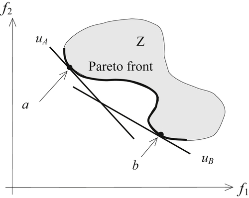
As shown in the above examples, the weighted-sum method is easy to use. If all weights are positive, the minimum of Eq. 5.9 is always a Pareto optimal. However, there are a few recognized difficulties with the weighted-sum method (Arora 2012). First, even with some of the methods discussed in the literature for determining weights, a satisfactory a priori weight selection does not necessarily guarantee that the final solution will be acceptable; one may have to resolve the problem with different weights. In fact, this is true of most weighted methods. The second problem is that it is impossible to obtain points on nonconvex portions of the Pareto optimal set in the criterion space. This is illustrated in Figure 5.8, which shows feasible criterion space and Pareto front of a two-objective problem. In this case, the Pareto front is a concave curve. Using the weighted-sum method, as discussed earlier, the converted objective function u(x) is a straight line in the f1-f2 plane. We select two sets of weights to create two new objective functions uA(x) and uB(x); both are straight lines with slopes determined by the respective weights, as shown in Figure 5.8. The two straight lines intersect the Pareto front at points a and b, respectively, resulting in two Pareto points. However, it is apparent that a straight line would never be able to reach the concave portion of the Pareto front. Therefore, the weighted-sum method is not able to find any solution located in the concave Pareto front. Another difficulty with the weighted-sum method is that varying the weights consistently and continuously may not necessarily result in an even distribution of Pareto optimal points and an accurate, complete representation of the Pareto optimal set.
An improvement to the weighted-sum is called the weighted-exponential sum, in which exponential p is added to objective functions as
![]() (5.14)
(5.14)
where and wi ≥ 0 ∀ i, and p > 0. In this case, p can be thought of as a compensation parameter; that is, a larger p implies that one prefers solutions with both very high and very low objective values rather than those with averaged values. In general, p may need to be very large to capture Pareto points in the nonconvex regions.
and wi ≥ 0 ∀ i, and p > 0. In this case, p can be thought of as a compensation parameter; that is, a larger p implies that one prefers solutions with both very high and very low objective values rather than those with averaged values. In general, p may need to be very large to capture Pareto points in the nonconvex regions.5.3.2.2. Weighted min–max method
The idea of the weighted min–max method (also called the weighted Tchebycheff method) is to minimize u(x), which represents the “distance” to an ideal utopia point in criterion space and is given as follows:
![]() (5.15)
(5.15)
A common approach to the treatment of Eq. 5.15 is to introduce an additional unknown parameter λ as follows:
![]() (5.16a)
(5.16a)
![]() (5.16b)
(5.16b)
The concept of solving the MOO problem defined Eq. 5.16 is illustrated in Figure 5.9 with two objective functions f1 and f2. First, the first term of Eq. 5.16b represents the length of a line originating from the utopia point and pointing in a direction, determined by the weights w1 and w2, toward the feasible criterion set. By minimizing λ, and hence the length of the line segment, the solution leads to a point on the Pareto front while keeping the design to be feasible.
The key advantage of the weighted min–max method is that it is able to provide almost all the Pareto optimal points, even for a nonconvex Pareto front. It is relatively well suited for generating the representative Pareto optimal front (with variation in the weights). However, this method requires the minimization of individual single-objective optimization problems to determine the utopia point, which can be computationally expensive. We demonstrate the weighted min–max method in Example 5.5.
5.3.2.3. Lexicographic method
With the lexicographic method, preferences are imposed by ordering the objective functions according to their importance or significance, rather than by assigning weights. After we arrange the objective functions by importance, the most important objective is solved first as a single-objective problem. The

EXAMPLE 5.5
Solve the same MOO problem of Example 5.3 using the weighted min–max method.
Solutions
Following the weighted min–max method, we need to find the utopia point first. In this case, the point is found at f0 = (−1, −1), as shown in the figure below, in which we recall that points a = (−1, 0) and b = (0, −1) represent the ends of the Pareto front—in this case, a 90° circular arc.
![]()
Hence, using the weighted min–max method, we are essentially solving the following single-objective optimization problem:
![]() (5.17a)
(5.17a)
![]() (5.17b)
(5.17b)

The single-objective problem can be solved, for example, using MATLAB (Script 4 in Appendix A). The solutions are obtained as x1 = x2 = −0.7071, and λ = 0.2929, which is on the Pareto front. We may adjust the weights to obtain other Pareto points. For example, if we choose w1 = 0.1 and w2 = 0.9, Eq. 5.17b becomes 0.1x1 + 0.9x2 + 1 − λ ≤ 0, and solutions are x1 = −0.1104, x2 = −0.9939, and λ = 0.0945, which is another Pareto point.
second objective is then solved as again a single-objective problem with an added constraint, defined as f1(x) ≤ f1(x1∗), in which x1∗ is the optimal solution of the first objective function. The process is repeated, in which optimal solution obtained in the previous step is added as a new constraint, and the sequence of single-objective optimization problems is solved, one problem at a time. Mathematically, the lexicographic method is defined as
![]() (5.18a)
(5.18a)
![]() (5.18b)
(5.18b)
where i represents a function's position in the preferred sequence, and fj( ) represents the minimum value for the jth objective function, found in the jth optimization problem. Note that after the first iteration, (j > 1), fj(xj∗) is not necessarily the same as the independent minimum of fj(x) because new constraints are introduced for each problem. The algorithm terminates once a unique optimum is determined. Generally, this is indicated when two consecutive optimization problems yield the same solution point. However, determining if a solution is unique (within the feasible design space S) can be difficult, especially with gradient-based solution techniques.
For this reason, often with continuous problems, this approach terminates after simply finding the optimum of the first objective f1(x). Thus, it is best to use a non-gradient-based solution technique with this approach. In any case, the solution is, theoretically, always Pareto optimal. We use an example problem (Example 5.6) similar to that of Example 5.2 to illustrate the concept of the method.
EXAMPLE 5.6
Solve the following MOLP problem using the lexicographic method, defined as
![]() (5.19a)
(5.19a)
![]() (5.19b)
(5.19b)
![]() (5.19c)
(5.19c)
![]() (5.19d)
(5.19d)
![]() (5.19e)
(5.19e)
![]() (5.19f)
(5.19f)
![]() (5.19g)
(5.19g)
Solutions
Note that the feasible set of the problem defined by Eqs. 5.19d–5.19g is identical to that of Example 5.2; that is, S = {x ∈ R2| gi(x) ≤ 0, i = 1,4}. In this problem, we have three objective functions f1, f2, and f3. We arrange the objective functions by importance as f1, f2, and f3. Therefore, we first optimize a single-objective problem for objective f1 as
![]() (5.19h)
(5.19h)

For this simple problem, we found the solution to this problem is all points in line segment between points B and C, as shown in the figure above. The function value is f1(x) = 4x1 + x2 = 10.02. Because the optimum solution is not unique, we continue by minimizing the second objective function f2 = 2x1 + x2 while adding the result of the first optimization problem to the constraint set:
![]() (5.19i)
(5.19i)
![]() (5.19j)
(5.19j)
Note that Eq. 5.19j is the additional constraint from the result of the first optimization. For the second optimization problem, we found the solution at point B, where f2 = 5.47, while f1 is unchanged satisfying the constraint function defined in Eq. 5.19j. Because the solution is unique, the process stops. The solution is found at point B, where f1 = 10.02, f2 = 5.47, and f3 = 3.21. Note that f3 was not even considered in the solution process because it is the least important objective among the three. If we change the importance order of the objective functions, we will most likely reach a different solution.
The advantages of the method include that it offers a unique approach to specifying preferences, it does not require that the objective functions be normalized, and it always provides a Pareto optimal solution. A few disadvantages on this method include that it can require the solution of many single-objective problems to obtain just one solution point, and it requires that additional constraints to be imposed. When there are more objective functions, the constraint set becomes large toward the end of the solution process.
5.3.3. Methods with A Posteriori Articulation of Preferences
In some cases, it is difficult for a designer to express preferences a priori. Therefore, it can be effective to allow the designer to choose from a palette of solutions. To this end, a number of methods aim at producing almost all the Pareto optimal solutions or a representative subset of the Pareto optimal. Such methods incorporate a posteriori articulation of preferences; they are called cafeteria or generate-first-choose-later approaches (Messac and Mattson 2002). Several methods belong to this category, such as the normal boundary intersection method (Das and Dennis 1998) and adaptive weighted-sum (Kim and de Weck 2006), to name a few. In addition, methods based on evolution algorithms (EA), such as the genetic algorithm to be discussed in Section 5.4, are considered a posteriori methods, although they solve the MOO problems in a much different way. In this subsection, we introduce one of the representative methods in this category, the normal boundary intersection (NBI) method.
5.3.3.1. Normal boundary intersection method
The normal boundary intersection method was developed in response to deficiencies in the weighted-sum approach. This method provides a means for obtaining an even distribution of Pareto optimal points, even with a nonconvex Pareto front of varying curvature. We use a two-objective problem shown in Figure 5.10 to illustrate the concept. The approach is formulated as follows:
![]() (5.20a)
(5.20a)
![]() (5.20b)
(5.20b)
where α is a point on the line segment AB, called the convex hull of individual minima (CHIM), which is also called the utopia line. Points A and B are the optimal points of the objective functions f1 and f2, respectively. n is a vector perpendicular to CHIM and pointing toward the Pareto front. The parameter β is a scalar to be maximized. Essentially, the concept of NBI is identifying a point α on the CHIM and searching a Pareto point along the n direction by maximizing parameter β. Because the constraint equation (Eq. 5.20b) ensures an attainable design point x in the feasible set S, maximizing β pushes the vector n to eventually intersect the Pareto front and yields a Pareto solution. If α points are chosen uniformly along the CHIM, a set of fairly evenly distributed Pareto points can be reasonably expected.
We use the same MOO problem of Example 5.3 to further illustrate the NBI method.

EXAMPLE 5.7
Solve the same MOO problem of Example 5.3 using the NBI method.
Solutions
In this case, we recall that the utopia point is found at f0 = (−1, −1), and points A = (−1, 0) and B = (0, −1). The CHIM line connecting points A and B is shown below. For this simple example, n can be found as n = [−1, −1]T. Therefore, using the NBI method, we are essentially solving the following single-objective optimization subproblem:
![]() (5.21a)
(5.21a)
![]() (5.21b)
(5.21b)

The single-objective problem can be solved, for example, using MATLAB (Script 5 in Appendix A). If we choose α = [−0.7, −0.3]T, the solution is obtained as x1 = −0.8782, x2 = −0.4782, and β = 0.1782, which is on the Pareto front. Note that β is the distance between α and the Pareto point found. We may pick another α point to obtain another Pareto point. For example, if we choose α1 = −0.5 and α2 = −0.5, the first term in Eq. 5.21b becomes [−0.5, −0.5]T, and solutions are x1 = −0.7071, x2 = −0.7071, and β = 0.2071.
![]() (5.21c)
(5.21c)
For problems with more than two objectives, the NBI method can be formulated in a more general form as
![]() (5.22a)
(5.22a)
![]() (5.22b)
(5.22b)
Here, Φ is a q × q payoff matrix with ith column composed of the vector f( ) − fo, where f() is the vector of objective functions evaluated at the minimum of the ith objective function. As a result, the diagonal elements of Φ are zeros. w is a vector of scalars such that
  and wi ≥ 0 ∀ i. n = −Φe, where e ∈ Rq is a column vector of ones in the criterion space. n is called a quasi-normal vector. Because each component of Φ is positive, the negative sign ensures that n points toward the origin of the criterion space. n gives the NBI method the property that for any w, a solution point is independent of how the objective functions are scaled. As w is systematically modified, the solution to Eq. 5.22 yields an even distribution of Pareto optimal points well representing the Pareto set.
and wi ≥ 0 ∀ i. n = −Φe, where e ∈ Rq is a column vector of ones in the criterion space. n is called a quasi-normal vector. Because each component of Φ is positive, the negative sign ensures that n points toward the origin of the criterion space. n gives the NBI method the property that for any w, a solution point is independent of how the objective functions are scaled. As w is systematically modified, the solution to Eq. 5.22 yields an even distribution of Pareto optimal points well representing the Pareto set.
We use a two-objective case shown in Figure 5.11 to illustrate the formulation geometrically. The right-hand side of Eq. 5.22b shifts the feasible criterion space Z such that the utopia point coincides with the origin of the two coordinate axes. The matrix Φ for this example is constructed as
 (5.23)
The vector n can be written as
 (5.24)
Hence, the constraint Eq. 5.22b is
 (5.25)
Note that the first term on the left-hand side of Eq. 5.25 (Φw) is nothing but a point on the CHIM line in the criterion space with axes  and
and  . The vector in the second term is the normal vector n in Eq. 5.20b. Therefore, the constraint equations in Eqs. 5.22b and 5.20b are very similar. The major difference is that in Eq. 5.22b the α points are generated by adjusting the vector w. For MOO problems with more than two objectives (q > 2), in which the CHIM becomes an utopia-hyperplane, Eq. 5.22b is more general in determining a set of uniformly distributed α points, as well as the normal vector n. As a result, uniformly distributed Pareto solutions can be expected.
In the Example 5.8, we revisit the pyramid example to illustrate more details on the NBI method formulated in Eq. 5.22.
EXAMPLE 5.8
Solve the pyramid problem using the NBI method.
Solutions
From Example 5.4, we have solved the two respective single-objective optimization problems for the optimal points and in the design space. The objective functions at these two design points are located in the criterion space f() = (A(), T()) and f() = (A(), T()) in the figure shown below. Hence, the utopia point is found at fo = (A(), T()) = (595.8, 865.3).

 (5.26a)
Plugging in the numbers, we have
 (5.26b)
Hence, using the NBI method, the problem is converted into a single-objective optimization as
![]() (5.26c)
(5.26c)
 (5.26d)
where S is the feasible space defined in Eq. 5.7. The single-objective problem can be solved, for example, using MATLAB (Script 6 in Appendix A).
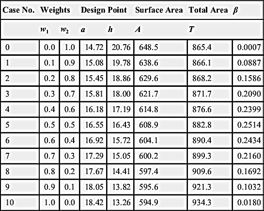
We choose w1 = 0.0, 0.1, …, 1.0 (and w2 = 1 − w1) and solved for these 11 cases. The results are listed in the table next page. Because the α points are selected uniformly along the CHIM by specifying a uniform increment 0.1 in w1 from 0 to 1, the Pareto points found from NBI are more evenly distributed. In this example, however, because the Pareto front is mild in geometry without significant changes in curvature, the advantage of the NBI is not apparent, and the results shown in the table below are similar to those in Example 5.4, in which weighted-sum method was employed.
| Case No. | Weights | Design Point | Surface Area | Total Area | β | ||
| w1 | w2 | a | h | A | T | ||
| 0 | 0.0 | 1.0 | 14.72 | 20.76 | 648.5 | 865.4 | 0.0007 |
| 1 | 0.1 | 0.9 | 15.08 | 19.78 | 638.6 | 866.1 | 0.0887 |
| 2 | 0.2 | 0.8 | 15.45 | 18.86 | 629.6 | 868.2 | 0.1586 |
| 3 | 0.3 | 0.7 | 15.81 | 18.00 | 621.7 | 871.7 | 0.2090 |
| 4 | 0.4 | 0.6 | 16.18 | 17.19 | 614.8 | 876.6 | 0.2399 |
| 5 | 0.5 | 0.5 | 16.55 | 16.43 | 608.9 | 882.8 | 0.2514 |
| 6 | 0.6 | 0.4 | 16.92 | 15.72 | 604.1 | 890.4 | 0.2434 |
| 7 | 0.7 | 0.3 | 17.29 | 15.05 | 600.2 | 899.3 | 0.2160 |
| 8 | 0.8 | 0.2 | 17.67 | 14.41 | 597.4 | 909.6 | 0.1692 |
| 9 | 0.9 | 0.1 | 18.05 | 13.82 | 595.6 | 921.3 | 0.1032 |
| 10 | 1.0 | 0.0 | 18.42 | 13.26 | 594.9 | 934.3 | 0.0180 |
5.3.4. Methods with No Articulation of Preference
Sometimes the designer cannot concretely define what he or she prefers. Consequently, this section describes methods that do not require any articulation of preferences. One of the simplest methods is the min–max method, formulated as
![]() (5.27)
(5.27)
The concept and formulation are straightforward. However, implementing Eq. 5.27 is not obvious. One possible approach is to introduce a new parameter β, which is to be minimized while requiring that all objective functions are no greater than β. Mathematically, the min–max problem can be formulated as
![]() (5.28a)
(5.28a)
![]() (5.28b)
(5.28b)
The following example (Example 5.9) illustrates the min–max method.
EXAMPLE 5.9
Solve the pyramid problem using the min–max method.
Solutions
Using the min–max method, the pyramid problem is formulated as
![]() (5.29a)
(5.29a)
 (5.29b)
where S is the feasible region defined in Eq. 5.7. The single-objective problem can be solved, for example, using MATLAB (Script 7 in Appendix A). The solution found is design point , at which a = 14.71, h = 20.80, surface area A = 649.0, total area T = 865.3, and β = 865.3. The parameter β = 865.3 is indeed the minimum because it is the minimum of the total area T. Although the solution does not minimize surface area A, reducing A cannot be done without increasing the total area T, in which β is no longer the minimum.
5.3.5. Multiobjective Genetic Algorithms
The solution techniques we discussed so far are mainly searching a single best solution representing the best compromise given the information from the designer. These techniques are called aggregating approaches because they combine (or “aggregate”) all the objectives into a single one. Such techniques approximate the Pareto front by repeating the solution process by adjusting parameters that redefine the search, such as the weights in the weighted-sum method.
In contrast to these techniques, methods based on evolution algorithms, such as multiobjective genetic algorithms, support direct generation of the Pareto front by simultaneously optimizing the individual objectives. As in the single-objective optimization problem discussed in Chapter 3, genetic algorithms emulate the biological evolution process. A population of individuals representing different solutions is evolving to find the optimal solutions. The fittest individuals are chosen, with mutation and crossover operations applied, thus yielding a new generation (offspring).
Evolutionary algorithms seem particularly suitable to solving multiobjective optimization problems because they deal simultaneously with a set of possible solutions (or a population). This allows designers to find several members of the Pareto optimal set in a single run of the algorithm, instead of having to perform a series of separate runs. Additionally, genetic algorithms are less susceptible to the shape or continuity of the Pareto front (e.g., they can easily deal with discontinuous or concave Pareto fronts), which are the two issues for mathematical programming techniques.
In general, for multiobjective problems, genetic algorithms have the advantage of evaluating multiple potential solutions in a single iteration. They offer greater flexibility for the designer, mainly in cases where no a priori information is available, as is the case for most real-life multiobjective problems. However, the challenge is how to guide the search toward the Pareto optimal set, and how to maintain a diverse population in order to prevent premature convergence. In addition, as discussed in Chapter 3, genetic algorithms require a large amount of function evaluations. For complex problems that require significant computation time for function evaluations, such as problems involving nonlinear finite element analysis, methods other than genetic algorithms are more practical.
One of the first treatments of multiobjective genetic algorithms, called the vector-evaluated genetic algorithm (VEGA), was presented by Schaffer (1985). Although this method was surpassed by others soon after it was proposed, it has provided a foundation for later development. Many prominent algorithms have been developed in the past three decades, in which ranking was explicitly used in order to determine the probability of replication of an individual. Such methods are so-called Pareto-based approaches.
In this section, we first provide a general discussion on the Pareto-based approaches. Thereafter, we zoom in to one of the most popular Pareto-based approaches, called the nondominated sorting genetic algorithm (NSGA). NSGA was proposed by Srinivas and Deb (1994) and revised to NSGA II (Deb et al. 2002), with significant improvements on the efficiency of the sorting algorithm as well as on its niche technique. We also present an example of NSGA II implementation in MATLAB, followed by the pyramid example for illustration. Note that some aspects of the method presented are shared by many other multiobjective genetic algorithms.
5.3.5.1. Pareto-based approaches
Pareto-based approaches incorporate three major elements—ranking, niching mechanism, and elitist strategy—in addition to the common mutation and crossover techniques seen in genetic algorithms. Ranking determines the probability of replication of an individual. The basic idea is to find the set of nondominated individuals in the population. These are assigned the highest rank and eliminated from further contention. The process is then repeated with the remaining individuals until the entire population is ranked and assigned a fitness value. In conjunction with Pareto-based fitness assignment, a niching mechanism is used to prevent the algorithm from converging to a single region of the Pareto front. The elitist strategy provides a means for ensuring that Pareto optimal solutions are not lost. Mutation and crossover operations are then performed to create the next generation of individuals.
5.3.5.1.1. Ranking
A simple and efficient method assumes that the fitness value of an individual is proportional to the number of other individuals it dominates, as illustrated in Figure 5.12. In Figure 5.12a, point 2 dominates six other individuals (points 3, 5, 6, 7, 9, and 10) because the objective function values at this point are less than those of the six points it dominates. Therefore, point 2 is assigned a higher fitness, and hence the probability of selecting this point is higher than, for example point 8, which only dominates two individuals (points 9 and 10).

Another version is the nondominated sorting genetic algorithm, which uses a layered classification technique, as illustrated in Figure 5.12b. In Figure 5.12b, a layered classification technique is used whereby the population is incrementally sorted using Pareto dominance. Individuals in set A have the same fitness value, which is higher than the fitness of individuals in set B, which in turn are superior to individuals in set C. All nondominated individuals are assigned the same fitness value. The process is repeated for the remainder of the population, with a progressively lower fitness value assigned to the nondominated individuals.
5.3.5.1.2. Niche techniques
A niche in genetic algorithms is a group of points that are close to each other, typically in the criterion space. Niche techniques (also called niche schemes, niche mechanism, or the niche-formation method) are methods for ensuring that a set of designs does not converge to a niche. Thus, these techniques foster an even spread of points in the criterion space. Genetic multiobjective algorithms tend to create a limited number of niches; they converge to or cluster around a limited set of Pareto optimal points. This phenomenon is known as genetic or population drift; niche techniques force the development of multiple niches while limiting the growth of any single niche.
Fitness sharing is a common niche technique. The basic idea of which is to penalize the fitness of points in crowded areas, thus reducing the probability of their survival for the next iteration. The fitness of a given point is divided by a constant that is proportional to the number of other points within a specified distance in the criterion space, thus reducing its fitness value and lowering its chance to survive for the next iteration. In this way, the fitness of all points in a niche is shared in some sense—thus the term “fitness sharing.”
5.3.5.1.3. Elitist strategy
Elitist strategy provides a means for ensuring that Pareto optimal solutions are not lost. It functions independently of the ranking scheme. Two sets of solutions are stored: a current population and a tentative set of nondominated solutions, which is an approximate Pareto optimal set. In each iteration, all points in the current population that are not dominated by any points in the tentative set are added to the tentative set. Then, the dominated points in the tentative set are discarded. After crossover and mutation operations are applied, a user-specified number of points from the tentative set are reintroduced into the current population. These are called elite points. In addition, q points with the best values for each objective function can be regarded as elite points and preserved for the next generation. Recall that q is the number of objective functions.
5.3.5.2. Nondominated sorting genetic algorithm II
With the understanding of the basic elements in the GA-based approaches for MOO problems, we now discuss NSGA II.
In NSGA II, before selection is performed, the population is ranked on the basis of nondomination: all nondominated individuals are classified into one category to provide an equal reproductive potential for these individuals. Because the individuals in the first front have the maximum fitness value, they always get more copies than the rest of the population when the selection is carried out. Additionally, the NSGA II estimates the density of solutions surrounding a particular solution in the population by computing the average distance of two points on either side of this point along each of the objectives of the problem. This value is called the crowding distance. During selection, NSGA II uses a crowded-comparison scheme that takes into consideration both the nondomination rank of an individual in the population and its crowding distance. The nondominated solutions are preferred over dominated solutions; however, between two solutions with the same nondomination rank, the one that resides in the less crowded region is preferred. The NSGA II uses the elitist mechanism that consists of combining the best parents with the best offspring obtained. More details are described in the next section.
5.3.5.2.1. Nondominated sorting
One of the major computation efforts in performing the nondominated sorting involves comparisons. Each solution can be compared with every other solution in the population to find out if it is dominated. This requires q×(N − 1) comparisons for each solution, where q is the number of objectives and N is the population size. The first round of sorting involves  comparisons, which is in the order of O(qN2).
comparisons, which is in the order of O(qN2).The results of the sorting are usually stored in an N×N matrix, in which each term indicates the dominance relation between two individuals in the population. In general, four scenarios need to be considered in terms of the feasibilities of the two individuals x and y being compared. First, if both x and y are feasible, then objectives at x and y are compared. If x dominates y, then the domination matrix donMat(x, y) = 1; else, if y dominates x, then donMat(x, y) = −1. Second, if x is feasible and y is infeasible, then donMat(x, y) = 1. Third, if x is infeasible and y is feasible, then donMat(x, y) = −1. Fourth, if both x and y are infeasible, then the constraint violations of x and y are compared. If violation at x is less than that of y, then donMat(x, y) = 1. Otherwise, donMat(x, y) = −1.
To further illustrate the idea, we use the example of population size N = 10 shown in Figure 5.12a. To simplify the discussion, we assume a nonconstrained problem. The matrix is set to zero initially. We pick point 2 to illustrate the process. As shown in Figure 5.12a, point 2 dominates points 3, 5, 6, 7, 9, and 10. Therefore, in the following matrix, entries (2, 3), (2, 5), (2, 6), (2, 7), (2, 9), and (2, 10) are set to 1. The entries (3, 2), (5, 2), (6, 2), (7, 2), (9, 2), and (10, 2) are set to −1. By going over the comparisons, the domination matrix can be constructed, as shown in Figure 5.13.
As proposed by Deb et al. (2002), for each individual we calculate two entities: (1) domination count np, the number of solutions that dominate the solution p, p = 1, N; and (2) Dp, a set of individuals that the solution dominates. The count np can be found by adding the number of −1 of the pth column in the matrix. The set Dp can be created by collecting individuals with −1 along the pth row in the matrix. For example, for point 2, n2 = 0 and D2 = {3, 5, 6, 7, 9, and 10}. By checking the columns and rows of the domination matrix, Table 5.2 can be constructed.
All solutions in the first nondominated front will have their domination count as zero (np = 0). From Table 5.2, the first nondominated front is identified as ND1 = {1, 2, 4, 8}. Now, for each solution in ND1, we visit each member of its set Dp and reduce its domination count by 1. For example, for the second member of ND1 (point 2), the counts of its members in D2 become respectively, n3 = 3 − 1 = 2, n5 = 1, n6 = 1, n7 = 4, n9 = 2, and n10 = 6. In doing so, if for any member the domination count becomes zero (if none is 0, we pick the ones with the lowest integer), these members belong to the second nondominated front ND2. In this example, solutions 5 and 6 of D2 have the lowest count 1. After repeating the same process for the remaining solutions 1, 4, and 8 in ND1, the second nondominated front is ND2 = {5, 6}. Now, the above procedure is continued with each member of ND2, and the third front is identified as ND3 = {7}. This process continues until all fronts are identified. Note that some individuals may not get counted, for example, 3, 9, and 10 in this case, which are dominated points. It is important that the first few nondominated fronts are identified accurately. In this example, the first two fronts, ND1 and ND2, are accurately identified as can be seen in Figure 5.12a.

Table 5.2
Domination Count np and the Set Dp Derived from the Domination Matrix
| Solution Point p | Solution p Dominates (Dp) | Solutions Dominate p | np |
| 1 | 3, 7, 10 | None | 0 |
| 2 | 3, 5, 6, 7, 9, 10 | None | 0 |
| 3 | None | 1, 2, 4 | 3 |
| 4 | 5, 6, 7, 9, 10 | None | 0 |
| 5 | 7, 10 | 2, 4 | 2 |
| 6 | 7, 10 | 2, 4 | 2 |
| 7 | None | 1, 2, 4, 5, 6 | 5 |
| 8 | 9, 10 | None | 0 |
| 9 | 10 | 2, 4, 8 | 3 |
| 10 | None | 1, 2, 4, 5, 6, 8, 9 | 7 |

5.3.5.2.2. Niche technique for diversity preservation
NSGA II employs a different niche technique to preserve the diversity of the Pareto solutions. This technique involves two factors: density-estimation metric and crowded-comparison operator.

Density estimation calculates an estimate of the density of points surrounding a particular solution in the population. The estimate calculates the average distance of two points on either side of this point along each of the objectives. This quantity serves as an estimate of the perimeter of the cuboid formed by using the nearest neighbors as the vertices (this is called the crowding distance). For example, in Figure 5.14, the crowding distance of the ith solution in its front (marked with solid circles) is the average side length of the cuboid (shown with a dashed box). The crowding-distance computation requires sorting the population according to each objective function value in ascending order of magnitude. Thereafter, for each objective function, the boundary solutions (solutions with smallest and largest function values) are assigned an infinite distance value. All other intermediate solutions are assigned a distance value equal to the absolute normalized difference in the function values of two adjacent solutions. This calculation is continued with other objective functions. The overall crowding-distance value is calculated as the sum of individual distance values corresponding to each objective. Note that each objective function is normalized before calculating the crowding distance.
The crowded-comparison operator (≺) guides the selection process at the various stages of the algorithm toward a uniformly spread-out Pareto optimal front. Assume that every individual in the population has two attributes:
1. Nondomination rank (irank)
2. Crowding distance (idistance).
We now define a partial order as
i ≺ j if (irank < jrank) or if (irank = jrank, idistance > jdistance).
That is, between two solutions with different nondomination ranks, we prefer the solution with the lower (better) rank. Otherwise, if both solutions belong to the same front, then we prefer the solution that is located in a lesser crowded region.
At the end of nondominated sorting, the individuals of the population of size N are sorted based on their rank. For the individuals of same rank, they are sorted by crowding distances.
5.3.5.2.3. Overall process
The overall NSGA II process consists of the creation of initial population and design iterations. Initially, a random parent population P0 of size N is created. Function evaluations of objectives and constraints are carried out for each of the N individuals. The population is sorted based on the nondomination and crowding distance, as discussed above.
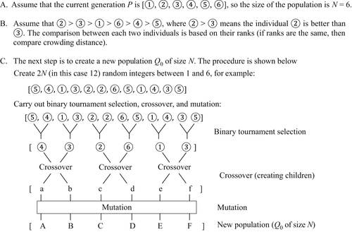
At first, the usual binary tournament selection, recombination, and mutation operators are used to create an offspring population Q0 of size N. The procedure is as follows. Function evaluations and nondominated (and crowding distance) sorting are performed. Then, a binary tournament selection is carried out to select the best N individuals. These N individuals go through crossover and mutation to generate a new population Q0 of size N. An example of these steps is shown in Figure 5.15 for illustration, in which N = 6 is assumed.
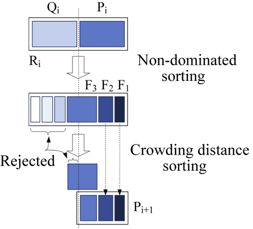
Because elitism is introduced by comparing the current population with the previously found best nondominated solutions, the procedure is different after the initial generation. We describe the ith generation of the algorithm. First, a combined population Ri = Pi ∪ Qi is formed. The population is of size 2N. Then, the population is sorted according to nondomination (and crowding distance). Because all previous and current population members are included in Ri, elitism is ensured. Now, solutions belonging to the best nondominated set F1 are of best solutions in the combined population (see Figure 5.16) and must be emphasized more than any other solution in the combined population. If the size of F1 is smaller than N, we choose all members of the set F1 for the new population Pi+1. The remaining members of the population Pi+1 are chosen from subsequent nondominated fronts in the order of their ranking. Thus, solutions from the set F2 are chosen next, followed by solutions from the set F3, and so on. This procedure is continued until no more sets can be accommodated. Say that the set  is the last nondominated set beyond which no other set can be accommodated. In general, the count of solutions in all sets from F1 to would be larger than the population size. To choose exactly N population members, we sort the solutions of the last front using the crowded-comparison operator in descending order and choose the best solutions needed to fill all population slots. This procedure is also shown in Figure 5.16. The new population Pi+1 of size N is now used for selection, crossover, and mutation to create a new population Qi+1 of size N.
5.3.5.3. Sample MATLAB implementation
In this section, we review a sample implementation of NSGA II written in MATLAB, and then we use this code to solve the pyramid example for illustration. The code is available for download at either its original site (www.mathworks.com/matlabcentral/fileexchange/31166-ngpm-a-nsga-ii-program-in-matlab-v1-4) or from the book's companion site. The zipped file consists of a set of MATLAB files and three folders. The doc folder includes a license file and a user manual. The other two folders, TP_NSGA2 and TP_R-NSGA2, include test problems that come with the code. Readers may download the code to go over some of the exercises at the end of this chapter.
There are two MATLAB files that users will have to create: one contains the input parameters, such as the number of objectives, whereas the other defines the objective and constraint functions. Once the two MATLAB files are created, we run the file with input parameters in MATLAB. The code searches for solutions at the Pareto front following the NSGA II algorithm discussed above. During the solution process, the code shows a list of generations, plots the solutions, and provides a summary on the status of the optimization, as shown in Figure 5.17.
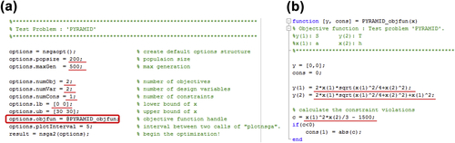
To solve the pyramid example using the code, we first create the two needed files and name them, respectively, PYRAMID.m and PYRAMID_objfun.m. The contents of these two files are shown in Figure 5.18. Note that the name of the function needs to match that defined in PYRAMID.m. In this case, the name of the function must be options.objfun = @PYRAMID_objfun, as circled in red in Figure 5.18a.
As shown in Figure 5.18a, the inputs of the pyramid example include the following:
• Population size: 200
• Number of generation: 500
• Number of objective functions: 2
• Number of design variables: 2
• Number of constraints: 1
• Lower bounds of design variables: 0 for the two design variables
• Upper bounds of design variables: 30 for the two design variables
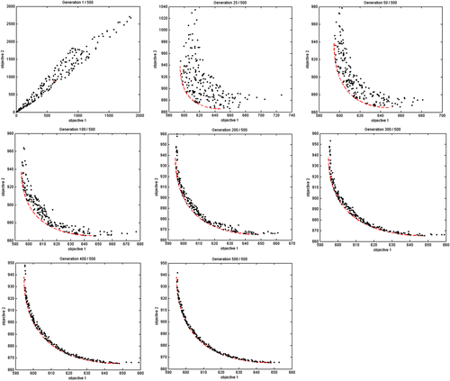
The MATALB script PYRAMID.m is called to start the optimization process. Results of a number of iterations are graphed in Figure 5.19, in which the red dotted line represents the Pareto front. As seen in Figure 5.19, the solutions converge rapidly to the Pareto front at the 200th iteration. At the last iteration (500), the Pareto front is well captured.

In general, the genetic algorithms successfully address the limitations of the classical approaches when generating the Pareto front. Because they allow concurrent exploration of different points of the Pareto front, they can generate multiple solutions in a single run. The optimization can be performed without a priori information about objectives relative importance. These techniques can handle ill-posed problems with incommensurable or mixed-type objectives. They are not susceptible to the shape of the Pareto front. Their main drawback is performance degradation as the number of objectives increases. Furthermore, they require additional parameters such as crossover fraction and mutation fraction, which need to be tweaked to improve the performance of the algorithms.
..................Content has been hidden....................
You can't read the all page of ebook, please click here login for view all page.