The advantage of academic codes is that they offer in general more choices of optimization techniques than commercial software packages; for example, more than 30 optimization algorithms (including single-objective and multiobjective) of different categories (gradient-based methods, genetic algorithms, etc.) are currently available in jMetal. Moreover, the algorithm libraries in most academic software programs can be constantly updated and expanded by incorporating new modules or optimization codes contributed by users. However, because most of such software tools are intended for academic use in support of testing and research, they are usually neither well-maintained nor advertised. As a result, they tend to be less flexible in coupling with third-party engineering software (such as CAD and CAE systems), and in most cases can only be used for solving simple optimization problems with known explicit expressions of the objective and constraint functions. In addition, these academic optimization tools often require the knowledge of certain programming languages (such as MATLAB), and their graphical user interfaces, if any, are not as user-friendly as those of commercial software.

A well-known multiobjective optimization tool for teaching and academic purposes is the NIMBUS system, developed by University of Jyväskylä. NIMBUS is a free web-based interactive tool that is capable of handling both differentiable and nondifferentiable single-objective and multiobjective optimization problems subject to nonlinear and linear constraints. The central idea of NIMBUS is to first find one Pareto optimum, and then generate additional solutions on the Pareto front based on the inputs from the user, including which of the objectives should be optimized most and what the limits of the objectives are. In other words, the optimization process is directed by the user. In NIMBUS, this interactive process is called a classification, and the optimal solutions obtained in this way effectively reflect the user's preferences.

The NIMBUS system is intuitive and easy for a novice to use. Because it operates via the Internet, no software needs to be downloaded. A simple tutorial example is available at wwwnimbus.it.jyu.fi/N4/tutorial/index.html. Now, we use the pyramid example to demonstrate the basic capabilities of NIMBUS. As shown in Figure 5.24a, we first enter the expressions of the objective and constraint functions, then identify the bounds of design variables (x1, x2, f1, and f2 correspond respectively to the two design variables a and h and the two objectives A and T in the pyramid example). Note that a starting point (initial design) is required (in this case, we choose a = 15 and h = 15) to initiate the optimization. The first solution obtained is shown in Figure 5.24b (A = 608.3, T = 883.5), which represents the black dot on the Pareto front (Figure 5.25a). The points A^∗ (594.8, 938.2) and T^∗ (649.0, 865.3) corresponding to the minimum of individual objectives are also calculated automatically, and are listed under the first solution, as shown in Figure 5.24b.

The next step is classification. As can be seen in Figure 5.24b, a group of buttons to the right of the first solution allow us to choose the “class” for each objective function. In this case, we choose “>” for f1 (objective function A) and “<” for f2 (objective function T), which implies our preference—further minimizing f2 based on the current solution while allowing f1 to change freely. Alternatively, if, for example, “≥” is chosen for f1, then a value needs to be assigned as the maximum allowed value for f1 when minimizing f2. The two new solutions (alternatives 2 and 3) generated according to the classification information are shown in Figure 5.25b. Note that f2 has been minimized to its lower bound in alternative 3. We then choose alternatives 1 and 3 to create five more Pareto solutions between the two (Figure 5.25b), and the results are listed in Figure 5.26a as alternatives 2 to 6.

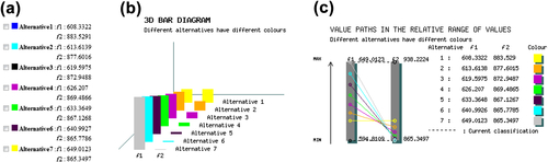
A number of solution visualization methods are available in NIMBUS, two of which are demonstrated in Figures 5.26b and c. In Figure 5.26c, each line represents a solution on the Pareto front (the seven solutions so far) between the first solution (alternative 1) and point T∗ (alternative 7). We can certainly continue the optimization process to obtain additional Pareto solutions.

Note that for nonacademic users, an implementation of NIMBUS that operates under several operating systems (such as Linux and Windows) is also available, known as IND-NIMBUS (ind-nimbus.it.jyu.fi). IND-NIMBUS has been tested with several industrial problems and can be connected with different simulators or modeling tools, such as MATLAB.

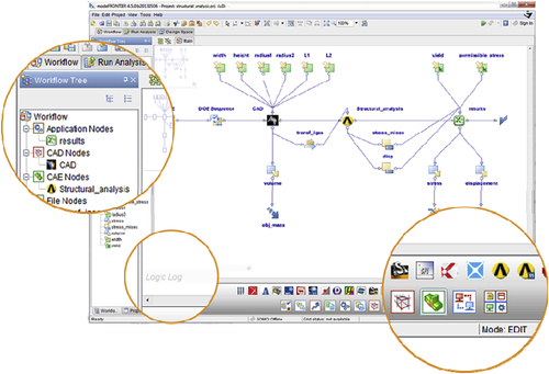
One of the key advantages of commercial codes is their ability to seamlessly couple with multiple third-party (commercial and in-house) engineering tools. Unlike the academic codes, these commercial software packages are designed to work with a wide variety of modeling and simulation software programs. Each of them can be thought of as an integration platform that enables the automation of a complex design simulation, and in the meantime offers optimization capabilities to support decision making. For example, the workflow environment in modeFRONTIER^® is able to formalize, drive, and manage individual steps, such as CAD modeling, computation fluid dynamics (CFD), finite element analysis (FEA), and so on, composing an engineering process through the integration of the most popular engineering solvers, while the data can be transferred automatically from one simulation to the next. Such communication between software is usually guaranteed by application protocol interfaces or automatic file exchange. Figure 5.27 shows a screen shot of the Workflow Editor in modeFRONTIER^®, and some of the third-party software supported in modeFRONTIER^®, including CAD, CAE, and generic applications, are listed in Table 5.4. Additional wizard style tools are also available in modeFRONTIER^® to achieve the coupling with other commercial tools or in-house codes. Some commercial optimization software, such as OPTIMUS^® and BOSS Quattro^®, also provide native interfaces with major CAE and FEA systems, broadening the basic capabilities of those engineering tools.

In addition to a strong connection with third-party applications, each of the commercial software packages mentioned above also bundles a collection of advanced optimization techniques for both single and multiobjective problems, ranging from gradient-based methods to genetic algorithms. For example, the multiobjective algorithms available in modeFRONTIER^® include multiobjective genetic algorithm (MOGA), adaptive range MOGA, multiobjective simulated annealing (MOSA), nondominated sorting genetic algorithm (NSGA II), multiobjective game theory, evolutionary strategies methodologies, and normal boundary intersection. Moreover, in modeFRONTIER^®, different algorithms can even be combined by the user in order to obtain hybrid approaches. For example, it is possible to combine the robustness of a genetic algorithm together with the accuracy of a gradient-based method, using the former for initial screening and the latter for refinements, so that the efficiency of the design cycle can be further enhanced. During optimization, these commercial software codes continuously update product parameters and extract relevant outputs from individual steps within the workflow until an optimal design is obtained. Because running a large number of simulations for optimization can be computationally expensive in practical engineering design, response surface methods (Jones 2001; Poles et al. 2008) are employed in most commercial software packages to accelerate the optimization process.

Another advantage of commercial optimization software over academic tools is that they often provide interactive result viewers to help users select the most suitable design. The alternatives obtained during optimization can be displayed in the forms of tables, charts, or two-dimensional (2D) and three-dimensional (3D) plots. As an example, the visualization of 2D and 3D Pareto fronts in OPTIMUS^® is shown in Figure 5.28. Usually, if the problem definition exceeds three dimensions, a 2D or 3D subspace can be selected, and parallel coordinate plots can be used to determine best designs out of the set of Pareto designs. Information other than the optimal solutions, such as the design space and sensitivity, can also be extracted and analyzed using the visualization tools incorporated in individual commercial optimization software (for example, see Figure 5.29).

Note that additional capabilities other than those discussed above are available in most commercial optimization software packages. For example, in modeFRONTIER^®, OPTIMUS^®, optiSLang^®, and Isight^®, robustness analysis and reliability analysis can be performed based on statistical methods, such as the Monte Carlo method, to deal with uncertainties that impact the optimization process. Also, modeFRONTIER^®, BOSS Quattro^®, and Isight^® allow users to run multiobjective optimization in parallel by evaluating more than one simulation at the same time using several local or remote processors.