Chapter 1. Arbitrage, Hedging, and the Law of One Price
...[Arbs] keep the markets honest. They bring perfection to imperfect markets as their hunger for free lunches prompts them to bid away the discrepancies that attract them to the lunch counter. In the process, they make certain that prices for the same assets in different markets will be identical.
—Peter L. Bernstein1
“Buy low, sell high.” “A fool and his money are soon parted.” “Greed is good.” All these adages illustrate the profit-oriented impulses of Wall Street traders, who stand ready to buy and sell. In pursuit of profits, undervalued assets are bought, and overvalued ones are sold. While risk is routinely borne in trading assets, most investors prefer to exploit mispriced assets with as little risk as possible. The goal is to enhance expected returns without adding risk. Think how seductive an investment that offers attractive returns but no risk is! One approach to identifying and profiting from misvalued assets is called arbitrage. Those who do it are called arbitrageurs or simply “arbs.”
Arbitrage is the process of buying assets in one market and selling them in another to profit from unjustifiable price differences. “True” arbitrage is both riskless and self-financing, which means that the investor uses someone else’s money. Although this is the traditional definition of arbitrage, use of the term has broadened to include often-risky variations such as the following:
• Risk arbitrage, which is commonly the simultaneous buying of an acquisition target’s stock and the selling of the acquirer’s stock.2
• Tax arbitrage, which shifts income from one investment tax category to another to take advantage of different tax rates across income categories.
• Regulatory arbitrage, which reflects the tendency of firms to move toward the least-restrictive regulations. An example is the historic tendency of U.S. commercial banks to move toward the least-restrictive regulator—state versus federal. Thus, as regulators in the past pursued a strategy of “competition in laxity,” banks sought to arbitrage regulatory differences.
• Pairs trading, which identifies two stocks whose prices have moved closely in the past. When the relative price spread widens abnormally, the stock with the lower price is bought, and the stock with the higher price is sold short.
• Index arbitrage, which establishes offsetting long and short positions in a stock index futures contract and a replicating cash market portfolio when the futures price differs significantly from its theoretical value.
Even though arbitrage may be motivated by greed, it is nonetheless a finely tuned economic mechanism that imposes structure on asset prices. This structure ensures that investors earn expected returns that are, on average, commensurate with the risks they bear. Indeed, prices and expected returns are not at rest unless they are “arbitrage-free.” Arbitrage provides both the carrot and the stick in efficiently operating financial markets.
Closely related to arbitrage is hedging, which is a strategy that reduces or eliminates risk and possibly locks in profits. By buying and selling specific investments, an investor can reduce the risk associated with a portfolio of investments. And by buying and selling specific assets, a target profit can be assured. Although all arbitrage strategies rely on hedging to render a position riskless, not all hedging involves arbitrage. “Pure” arbitrage is the riskless pursuit of profits resulting from mispriced assets. Hedging strategies seek to reduce, if not eliminate, risk, but do not necessarily involve mispriced assets. Thus, hedging does not purse profits.3
A guiding principle in investments is the Law of One Price. This states that the “same” investment must have the same price no matter how that investment is created. It is often possible to create identical investments using different securities or other assets. These investments must have the same expected cash flow payoffs to be considered identical. Indeed, the threat of arbitrage ensures that investments with identical payoffs are, at least on average, priced the same at a given point in time. If not, arbitrageurs take advantage of the differential, and the resulting buying and selling should eliminate the mispricing.
Similar to the Law of One Price is the Law of One Expected Return,4 which asserts that equivalent investments should have the same expected return. This is a bit different from the prior requirement that the same assets must have the same prices across markets. While subtle, this distinction will help you understand arbitrage in the context of specific pricing models.
The concepts of arbitrage, hedging, and the Law of One Price are backbones of asset pricing in modern financial markets. They provide insight into a variety of portfolio management strategies and the pricing of assets. This chapter explores the nature and significance of arbitrage and illustrates how it is used to exploit both mispriced individual assets and portfolios. It consequently provides a broad analytical framework to build on in subsequent chapters. For example, the next chapter illustrates arbitrage strategies in terms of the capital asset pricing model (CAPM) and the Arbitrage Pricing Theory (APT).
Why Is Arbitrage So Important?
True arbitrage opportunities are rare. When they are discovered, they do not last long. So why is it important to explore arbitrage in detail? Does the benefit justify the cost of such analysis? There are compelling reasons for going to the trouble.
Investors are interested in whether a financial asset’s price is correct or “fair.” They search for attractive conditions or characteristics in an asset associated with misvaluation. For example, evidence exists that some low price/earnings (P/E) stocks are perennial bargains, so investors look carefully for this characteristic along with other signals of value. Yet the absence of an arbitrage opportunity is at least as important as its presence! While the presence of an arbitrage opportunity implies that a riskless strategy can be designed to generate a return in excess of the risk-free rate, its absence indicates that an asset’s price is at rest. Of course, just because an asset’s price is at rest does not necessarily mean that it is “correct.” Resting and correct prices can differ for economically meaningful reasons, such as transactions costs.
For example, a $1.00 difference between correct and resting prices cannot be profitably exploited if it costs $1.25 to execute the needed transactions. Furthermore, sometimes many market participants believe that prices are wrong, trade under that perception, and thereby influence prices. Yet there may not be an arbitrage opportunity in the true sense of a riskless profit in the absence of an initial required investment. Thus, it is important to carefully relate price discrepancies to the concept of arbitrage because one size does not fit all.
Arbitrage-free prices act as a benchmark that structures asset prices. Indeed, understanding arbitrage has practical significance. First, the no-arbitrage principle can help in pricing new financial products for which no market prices yet exist. Second, arbitrage can be used to estimate the prices for illiquid assets held in a portfolio for which there are no recent trades. Finally, no-arbitrage prices can be used as benchmark prices against which market prices can be compared in seeking misvalued assets.5
The Law of One Price
Prices and Economic Incentives: Comparing Apples and Assets
We expect the same thing to sell for the same price. This is the Law of One Price. Why should this be true? Common sense dictates that if you could buy an apple for 25¢ and sell it for 50¢ across the street, everyone would want to buy apples where they are cheap and sell them where they are priced higher. Yet this price disparity will not last: As people take advantage, prices will adjust until apples of the same quality sell for the same price on both sides of the street. Furthermore, a basket of apples must be priced in light of the total cost of buying the fruit individually. Otherwise, people will make up their own baskets and sell them to take advantage of any mispricing.6 The arbitrage relationship between individual asset prices and overall portfolio values is explored later in this chapter.
The structure imposed on prices by economic incentives is the same in financial markets as in the apple market. Yet a different approach must be taken to determine what constitutes the “same thing” in financial markets. For example, securities are the “same” if they produce the same outcomes, which considers both their expected returns and risk. They should consequently sell for the same prices. Similarly, equivalent combinations of assets providing the same outcomes should sell for the same price. Thus, the criteria for equivalence among financial securities involve the comparability of expected returns and risk. If the same thing sells for different prices, the Law of One Price is violated, and the price disparity will be exploited through arbitrage. Thus, the Law of One Price imposes structure on asset prices through the discipline of the profit motive. Similarly, if stocks with the same risk have different expected returns, the Law of One Expected Return is violated.
Economic Foundations of the Law of One Price
The Law of One Price holds under reasonable assumptions concerning what investors like and dislike and how they behave in light of their preferences and constraints. Specifically, our analysis assumes the following:
• More wealth is preferred to less. Wealth enhancement is a more comprehensive criterion than return or profit maximization. Wealth considers not only potential returns and profits but also constraints, such as risk.7
• Investor choices should reflect the dominance of one investment over another. Given two alternative investments, investors prefer the one that performs at least as well as the other in all envisioned future outcomes and better in at least one potential future outcome.
• An investment that generates the same return (outcome) in all envisioned potential future situations is riskless and therefore should earn the risk-free rate. Lack of variability in outcomes implies no risk. Thus, strategies that produce riskless returns but exceed the risk-free return on a common benchmark, such as U.S. Treasury bills, must involve mispriced investments.
• Economic incentives ensure that two investments offering equivalent future outcomes should, and ultimately will, have equivalent prices (returns).
• The proceeds of a short sale are available to the investor. This assumption is easiest to accept for large, institutional investors or traders who may be considered price-setters on the margin. Even if this assumption seems a bit fragile, market prices generally behave as if it holds well enough.8 The nature and significance of short sales are discussed more later in this chapter.
Systematic, persistent deviations from the Law of One Price should not occur in efficient financial markets.9 Deviations should be relatively rare or so small as to not be worth the transactions costs involved in exploiting them. Indeed, when arbitrage opportunities do appear, those traders with the lowest transactions costs are likely to be the only ones who can profitably exploit them. The Law of One Price is largely—but not completely—synonymous with equilibrium, which balances the forces of supply and demand.
The Nature and Significance of Arbitrage
Arbitrage Defined
Arbitrage is the process of earning a riskless profit by taking advantage of different prices for the same good, whether priced alone or in equivalent combinations. Thus, due to mispricing, a riskless position is expected to earn more than the risk-free return. A true arbitrage opportunity exists when simultaneous positions can be taken in assets that earn a net positive return without exposing the investor to risk and, importantly, without requiring a net cash outlay. In other words, pure arbitrage requires no upfront investment but nonetheless offers a possible profit. The requirement that arbitrage not demand additional funds allows for the possibility that the position either generates an initial cash inflow or neither provides nor requires any cash initially. Consider the intuition behind this requirement. A positive initial outlay means that the arbitrage strategy is not self-financing. This would imply at least the risk that the initial investment could be lost, which is inconsistent with the no-risk requirement for the presence of an arbitrage opportunity.10
Arbitrage may be considered from at least two perspectives. First, arbitrage may involve the construction of a new riskless position or portfolio designed to exploit a mispriced asset or portfolio of assets. Second, arbitrage may involve the riskless modification of an existing asset or portfolio that requires no additional funds to exploit some mispricing. Both perspectives are considered in the arbitrage examples presented in Chapter 2, “Arbitrage in Action.”
The Relationship Between the Law of One Price and Arbitrage
If the Law of One Price defines the resting place for an asset’s price, arbitrage is the action that draws prices to that spot. The absence of arbitrage opportunities is consistent with equilibrium prices, wherein supply and demand are equal. Conversely, the presence of an arbitrage opportunity implies disequilibrium, in which assets are mispriced. Thus, arbitrage-free prices are expected to be the norm in efficient financial markets. The act of arbitraging mispriced assets should return prices to their appropriate values. This is because investors’ purchases of the cheaper asset will increase the price, while sales of the overpriced asset will cause its price to decrease. Arbitrage consequently reinforces the Law of One Price and imposes order on asset prices.
Hedging and Risk Reduction: The Tool of Arbitrage
Hedging Defined
A hedge is used to implement an arbitrage strategy. Thus, before we examine arbitrage more carefully, we must understand how a hedge works. We have all heard someone say that he or she did something just to “hedge a bet.” In a strict gambling sense, this implies that an additional bet has been placed to reduce the risk of another outstanding bet. The everyday connotation is that an action is taken to gain some protection against a potentially adverse outcome. For example, you may leave early for an appointment to “hedge your bet” that you’ll find a parking place quickly. Another example is a college student’s decision to pursue a double major because he doesn’t know what jobs will be available when he graduates.
In investment analysis, a hedging transaction is intended to reduce or eliminate the risk of a primary or preexisting security or portfolio position. An investor consequently establishes a secondary position to counterbalance some or all of the risk of the primary investment position. For example, an equity mutual fund manager would not get completely out of equities if the market is expected to fall. (Just think of the signal that would send to investors.) The risk of the manager’s long equity investments could be partially offset by taking short positions in selected equities, buying or selling derivatives, or some combination thereof.11 This secondary position hedges the equity portfolio by gaining value when the value of the equity fund falls. The workings of such hedges are discussed next.
Often, an investor establishes a long asset position that is subsequently considered too risky. The investor consequently decides to partially or completely offset that risk exposure by taking another investment position that offsets declines in the original investment’s value. A short position can be taken in the same asset that counterbalances the investor’s risk exposure. The hedging transaction may be viewed as a substitute for the investor’s preferred action in the absence of constraints that interfere with taking that action.12 The constraint could be something explicit, like a portfolio policy requirement (such as in a trust) that an investor maintain a given percentage of funds invested in a stock. Alternatively, it could be a self-imposed risk-tolerance constraint where the investor wants to keep a stock with a profit but feels compelled to offset all or part of the position’s risk using a hedging transaction. For instance, this could be motivated by tax treatment issues.
As noted, it is important to understand how hedging works before exploring its use in implementing arbitrage strategies. Thus, we’ll now explain how an investor constructs a hedge that holds a stock, locks in an established profit, and neutralizes risk.
Hedging Example: Protecting Profit on an Established Long Position
Investment Scenario and Expected Results of the Hedge
Consider a stock originally bought for $85 that has risen to $100. For our purposes, we’ll ignore commissions associated with buying and selling securities. What should the investor do if he is happy with the $15 profit on the investment but fears that the market may fall soon? The most obvious solution is to sell the stock and take the $15 profit now. However, what if the investor is unable or unwilling to sell the stock now but still wants to lock in the profit? Perhaps the investor wants to delay realizing a taxable gain until next year or wants to stretch an existing short-term gain into a long-term gain.13 The investor could sell short the stock at its current price of $100, which would protect against any loss of the $15 profit. Any drop in the value of the stock would then be offset by an equal appreciation in the value of the outstanding short position. The investor has a $15 profit that could be realized by selling the stock now. However, the investor substitutes a hedging short sale transaction for the direct sale of the long position. This substitute transaction protects the profit while maintaining the original long stock position.14
The Effect of Price Changes on Hedge Profitability
What would happen if the price of the stock falls from $100 to $90? Remember that the short position locks in the proceeds from selling at $100. If the price falls to $90, the stock can be purchased at that price and returned to the lending broker, thereby generating a profit of $10. However, the profit on the long position is reduced by $10 due to the price decline. Thus, there would be no net deviation from the established profit of $15.
The hedge brings both good and bad news. The good news is that the $15 profit is locked in without risk. Yet the bad news is that the investor cannot profit further from any increase in the stock price beyond $100. This is because a price increase would raise the value of the long position but would also bring offsetting losses on the short position.
What if the price moves from $100 to $110? The profit on the long position increases from $15 to $25 a share, but the short position loses $10 a share. From a cost/benefit perspective, the “benefit” of locking in the established $15 profit comes at the “cost” of eliminating the ability to gain even greater profits. In other words, the benefit of the hedge is the floor that it places on potential losses, and its (opportunity) cost is the ceiling placed on the position’s maximum profit. This makes sense in light of the risk/return trade-off. The hedge reduces or eliminates risk and therefore reduces or eliminates subsequent expected returns. Table 1.1 summarizes the potential outcomes associated with the hedge. In this scenario, an investor buys 100 shares of stock at $85 a share, and it is now selling for $100. The investor wants to lock in the $15 profit without selling the stock. For the hedging transaction, the investor sells short 100 shares at $100 a share.
Table 1.1. The Good and Bad News of Hedging
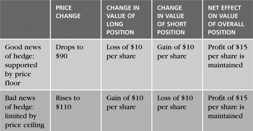
Figure 1.1 portrays the results graphically.
Figure 1.1. Hedging to Protect Profits
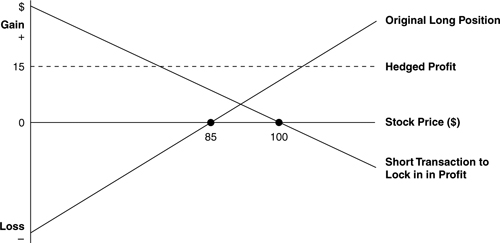
The profit/loss potential of the long position originally established by buying at $85 intersects with the vertical axis at –$85 and intersects with the horizontal break-even axis at +$85. This indicates that the maximum loss is $85, which occurs if the stock price falls to zero. Furthermore, the break-even price of $85 is obtained if the price remains at its original purchase price. The positive, upward-sloping profit/loss line indicates that profits increase dollar-for-dollar as the stock’s price rises above the original purchase price of $85. Similarly, profits fall dollar-for-dollar as the stock’s price falls below the original purchase price. The maximum gain is, at least in theory, infinite.
The profit/loss potential of the short position established by selling borrowed shares at $100 intersects with the vertical axis at +$100 and intersects with the horizontal break-even axis at $100. This indicates that the maximum gain is +$100, which occurs if the stock price falls to zero. The break-even price of $100 occurs if the price remains at its original level. The negative, downward-sloping profit/loss line indicates that profits increase dollar-for-dollar as the stock’s price falls below the original short sales price of $100, and profits decline dollar-for-dollar as the stock’s price rises above the price at which the shares were sold short. The maximum loss is theoretically, but soberingly, infinite.
The most dramatic result portrayed in Figure 1.1 is the horizontal hedged profit line, which shows that profits are fixed at $15 per share regardless of where the stock’s price ends up. The horizontal line results from offsetting the upward-sloping long position profit/loss line against the downward-sloping short position profit/loss line. The opposite slopes of the two lines imply that when one position is losing money, the other is making money. Thus, the horizontal hedging profit line reflects the risk-neutralizing effect of combining the short (hedging) transaction with the investor’s original long position in the stock. Gains and losses on the two individual positions cancel each other out, thereby resulting in a fixed profit of $15 per share. This $15 profit is the difference between the original purchase price of the stock at $85 and the price at which it was sold short at $100.
The Rate of Return on Hedged Positions and Its Relationship to Arbitrage
In the preceding example, the investor locks in an ex post (afterthe-fact) 17.65% return ($15/$85) through a hedge. The investor has effectively removed the position from the market and has an expected zero rate of return from that time on. Importantly, the position is riskless after the given 17.65% return is generated, and no deviation above or below that return is possible after the hedge is in place. However, insufficient data are given in the example to judge whether the ex post return of 17.65% is appropriate to the risk of the investment.
An investor cannot engage in arbitrage that profitably exploits mispriced investments without adding risk unless he can hedge. This is because the hedge is the means whereby the arbitrage strategy is rendered riskless. Hedging is an essential mechanism that allows arbitrage to structure asset prices.
Mispricing, Convergence, and Arbitrage
Arbitrage exploits violations of the Law of One Price by buying and selling assets, separately or in combination, that should be priced the same but are not. Implicit in an arbitrage strategy is the expectation that the prices of the misvalued assets will ultimately move to their appropriate values. Indeed, arbitrage should push prices to their appropriate levels. Thus, an arbitrage strategy has two key aspects: execution and convergence. Execution includes how the arbitrage opportunity is identified in the first place, how the strategy is put together, how it is maintained over its life, and how it is ultimately closed out. Convergence is the movement of misvalued asset prices to their appropriate values.15 Of particular importance are the time frame over which convergence is expected to occur and the process driving the convergence. These two are the primary factors that determine the design of the appropriate arbitrage strategy in a given situation.
The processes driving convergence fall into two categories: mechanical or absolute, and behavioral or correlation. A mechanical or absolute convergence process has an explicit link that forces prices to converge over a well-defined time period. An example is index arbitrage, in which the futures price of an index is mechanically linked to the spot (cash) value of the index through the cost-of-carry pricing relation. This is examined in Chapter 3, “Cost of Carry Pricing.” In index arbitrage, the convergence time period is deterministically dictated by the delivery/expiration date of the index futures contract.
A behavioral or correlation convergence process exists when there is historical evidence of a systematic relationship or a correlation in the behavior of the assets’ prices. However, the mispriced assets fall short of being linked mechanically. An example of a behavioral or correlation convergence process is pairs trading. Pairs trading identifies two stocks that have historically tended to move closely, as measured by the average spread between their prices. It is common to identify pairs of stocks that are highly correlated in large part due to being in the same industry. The essence of this strategy is to identify pairs whose spreads are significantly higher or lower than usual and then sell the higher-priced stock and buy the lower-priced stock under the expectation that the spread will eventually revert to its historical average. Thus, pairs trading relies on an estimated correlation and projected convergence toward the historical mean spread. Importantly, no mechanical link guarantees this convergence, and no deterministic model indicates how long such convergence should take. Although they are commonly referred to as arbitrage, behavioral/correlation convergence process-based strategies are not true arbitrage, because they can be quite risky. This book is concerned primarily with mechanical/absolute convergence process-based arbitrage because that is the fertile soil from which modern finance has grown.
Identifying Arbitrage Opportunities
Arbitrage Situations
Arbitrage opportunities exist when an investor either invests nothing and yet still expects a positive payoff in the future or receives an initial net inflow on an investment and still expects a positive or zero payoff in the future.18
This appeals to the commonsense expectation that money must be invested to result in a positive payoff. Furthermore, if you receive money upfront, you expect at the least to pay it back and certainly do not expect the investment to produce positive payoffs in the future. It is also reasonable to expect the value of a portfolio of assets to properly reflect the prices of the underlying components of that portfolio. Thus, the situations described in this chapter indicate arbitrage opportunities in which deviations from the Law of One Price can potentially be exploited. Any one of these conditions is sufficient for the presence of an arbitrage opportunity. Consider the following examples, which indicate the presence of an arbitrage opportunity.
Arbitrage When “Whole” Portfolios Do Not Equal the Sum of Their “Parts”19
What if the price of a portfolio is not equal to the sum of the prices of the assets when purchased separately and combined into an equivalent portfolio? This summons the earlier image of a basket of fruit selling for a price different from the cost of buying all its contents individually. More specifically, if fruit basket prices are too high, people will buy individual fruit and sell baskets of fruit. They would consequently “play both ends against the middle” to make a profit.
This situation could occur when commodities or securities are sold both separately and as a “packaged” bundle. For example, the Standard & Poor’s 500 Composite Index (S&P 500) is a portfolio consisting of 500 U.S. stocks that can be traded as a package using an SPDR.20 Of course, the stocks can also be traded individually. Thus, an arbitrage opportunity would exist if the S&P 500-based SPDR sold at a price different from the cost of separately buying the 500 stocks comprising the index.
Consider what happens if this condition is not satisfied for a two-stock portfolio consisting of one share of Merck (MRK) selling at $31.46 and one share of Yahoo (YHOO) selling at $34.02. If the price of the equal-weighted portfolio differs from $31.46 + $34.02 = $65.48, an investor could profit without assuming any risk.
The two possible imbalances are as follows:
Price portfolio (MRK + YHOO) > $31.46 + $34.02
or
Price portfolio (MRK + YHOO) < $31.46 + $34.02
In the first case, the portfolio is overpriced relative to its two underlying components. In the second case, the portfolio is underpriced relative to its components. More specifically, assume in the first case that the portfolio sells for $75.00 and in the second case that the portfolio sells for $55.00. We expect that the sum of the prices of MRK and YHOO will equal the price of the portfolio at some time in the future. However, in light of the earlier discussion of convergence, we must admit that because there was mispricing to begin with, there is no certainty that the relevant prices will equalize in the future. We assume that such convergence will occur eventually.
If the price of the portfolio is $75.00 and therefore exceeds the costs of buying MRK and YHOO individually, the strategy is to buy a share of MRK for $31.46 and a share of YHOO for $34.02 separately because they are cheap relative to the price of the portfolio. To finance the purchases, it is necessary to sell short the portfolio for $75.00 at the same time. Because the price of the portfolio exceeds the cost of buying each of its members separately, selling the portfolio short generates sufficient money to purchase the stocks individually. The strategy consequently is self-financing. It generates a net initial cash inflow of $75.00 – $65.48 = $9.52.
Yet what will the net long and short positions yield in the future? You will have to return the portfolio at some time in the future to cover the short position, which involves a cash outflow to buy the portfolio. However, you already own the shares that constitute that portfolio. Thus, subsequent moves in the prices of MRK and YHOO are neutralized by the offsetting changes in the value of the portfolio consisting of the same two stocks. Thus, the net cash flow in the future is zero.
What does this mean? It means that you could generate an initial cash inflow of $9.52—that is like getting a loan you never have to repay! This cannot last, because everyone would pursue this strategy. Indeed, investors would pursue this with as much money as possible! Ultimately the increased demand to buy MRK and YHOO would put upward pressure on their prices, and the demand to sell short the portfolio would put downward pressure on its price. Consequently, an arbitrage-free position will ultimately be reached in which the price of the portfolio equals the sum of the prices of the assets when purchased separately.
To reinforce this result, consider the other imbalance, in which the price of the portfolio is only $55.00, which is less than the costs of buying MRK and YHOO individually for a total of $65.48. The strategy is to sell short a share of MRK for $31.46 and to sell short a share of YHOO for $34.02 separately because they are expensive relative to the price of the portfolio at $55.00. Similarly, you would buy the portfolio for $55.00 because it is cheap relative to its underlying components.
It is obvious that selling short the two stocks individually generates more cash inflow than the cash outflow required to purchase the portfolio. Thus, the investment generates an initial positive net cash inflow of $65.48 – $55.00 = $10.48. As in the case just evaluated, it is important to consider the cash flow at termination of the investment positions in the future. Some time in the future you will have to return the shares of MRK and YHOO to cover the short sale of each stock, which involves the cash outflow to buy each of the two stocks. However, you already own the portfolio, which consists of a share each of MRK and YHOO. Thus, subsequent moves in the prices of the long positions in MRK and YHOO are neutralized by the equivalent, mirroring price moves of the same stocks within the short portfolio. Consequently, the net cash flow in the future is zero. As observed with the other imbalance, you can effectively borrow money that never has to be paid back! This indicates an arbitrage opportunity and shows why only arbitrage-free asset and portfolio prices persist.
Arbitrage When Investing at Zero or Negative Upfront Cost with a Zero or Positive Future Payoff
An arbitrage opportunity can be identified based on the relationship between the initial and future cash flows of a portfolio formed by an investor who buys and sells the component assets separately. Consider the case in which putting together a portfolio of individual assets generates either a zero net cash flow or a cash inflow initially and yet that portfolio produces a positive or zero cash inflow in the future. This situation produces an arbitrage opportunity because everyone would want to replicate the portfolio at no cost or even receive money up-front and also receive money or not have to pay it back in the future.
Consider three individual assets that can be purchased separately and as a portfolio. Table 1.2 portrays the cash flows to be paid by each of the three assets and the portfolio at the end of the period as well as their prices at the beginning of the period. The future cash flow payoffs are also presented.
Table 1.2. Example Identifying an Arbitrage Opportunity
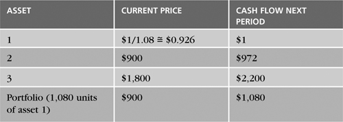
Table 1.2 shows that an arbitrage opportunity exists. Remember that an arbitrage opportunity is present if the price of a portfolio differs from the cost of putting together an equivalent group of securities purchased separately. In this example, the portfolio of 1,080 units of asset 1 can be purchased more cheaply than if 1,080 units of asset 1 are purchased separately. Specifically, it would cost $1,000 or 1,080 (0.926) to buy 1,080 units of asset 1 individually, while a portfolio of 1,080 units of asset 1 is priced at only $900. Thus, the “whole” portfolio is not equal to the sum of its “parts.”
The arbitrage strategy is to sell short 1,080 units of asset 1 for $1,000 now to finance the purchase of one (undervalued) portfolio that contains 1,080 units of asset 1 for only $900. The resulting current cash inflow is $1,000 – $900 = $100. No cash inflow or outflow would occur at the end of the period, because you would hold a portfolio of asset 1 that is worth $1,080, which is the same value you must return to cover the short position in 1,080 individual units of asset 1. Thus, $100 is generated upfront, and nothing must be returned. This is either a dream come true or an arbitrage opportunity—one and the same. Obviously, investors would pursue this opportunity on the largest possible scale.
Another arbitrage condition is satisfied using assets 2 and 3. The current value of the portfolio formed by buying and selling these two assets separately is nonpositive, which means that either there is no initial cash flow or there is an initial cash inflow. Thus, the portfolio either is costless or produces a positive cash inflow when established and yet still generates cash at the end of the period. Using the data in Table 1.2, the arbitrage portfolio is formed by selling short two units of asset 2 and buying one unit of asset 3. The initial outlay would be –2($900) + 1($1,800) = 0. Notwithstanding the zero cost of forming the portfolio, at the end of the period the cash flow is expected to be –2($1,800) + 1($2,200) = $400. Thus, an arbitrage opportunity exists because the strategy is costless but still produces a future positive cash inflow. The portfolio consequently is a proverbial money machine that investors would exploit on the greatest scale available to them.
Market Implications of Arbitrage-Free Prices
The conditions required for the presence of an arbitrage opportunity imply that their absence also places a structure on asset prices. As noted, prices are at rest when they preclude arbitrage. Specifically, arbitrage-free prices imply two properties. First, asset prices are linearly related to cash flows. Known as the value additivity property, this implies that the value of the whole portfolio is simply the added values of its parts. Thus, the value of an asset should be independent of whether it is purchased or sold individually or as a member of a portfolio. Second, any asset or portfolio that has positive cash flows in the future must necessarily have a positive current price. This is often referred to as the dominance criterion. Thus, the absence of arbitrage opportunities places a structure on asset prices.
Summary
This chapter explored the relationship between arbitrage, hedging, the Law of One Price, the Law of One Expected Return, and the structure of asset prices. The same thing is expected to sell for the same price. This is the Law of One Price. Securities are the same if they produce the same outcomes, which encompass both their expected returns and risk. Similarly, equivalent combinations of assets providing the same outcomes should sell for the same prices. Thus, the criteria for sameness or equivalence among financial securities involve the comparability of expected returns and risk. If the same thing sells for different prices, the Law of One Price is violated, and the price disparity can be exploited if transactions costs are not prohibitive. Thus, the Law of One Price imposes structure on asset prices through the discipline of the profit motive. Similarly, equivalent securities and portfolios must have the same expected return. This is the Law of One Expected Return.
If the Law of One Price defines the resting place for an asset’s price, arbitrage is the action that draws prices to that resting place. Arbitrage is defined as the process of earning a riskless profit by taking advantage of different prices or expected returns for the same asset, whether priced alone or in equivalent combinations of assets.
True arbitrage must be riskless. The ability to hedge is a necessary condition for arbitrage because it can eliminate risk. Thus, a hedging transaction is intended to reduce or eliminate the risk of a primary security or portfolio position. An investor consequently establishes a secondary position that is designed to counterbalance some or all of the risk associated with another investment position.
This chapter identified the conditions associated with the presence of an arbitrage opportunity. An arbitrage opportunity exists when an investor can put up no cash and yet still expect a positive payoff in the future and when an investor receives an initial net inflow but can still expect a positive or zero payoff in the future. An arbitrage opportunity is also present when the value of a portfolio of assets is not equal to the sum of the prices of the underlying securities composing that portfolio.
The absence of arbitrage opportunities is consistent with equilibrium prices. Thus, arbitrage-free prices are expected to be the norm in efficient financial markets. The act of arbitraging mispriced assets should return prices to appropriate values. Arbitrage consequently reinforces the Law of One Price or the Law of One Expected Return and imposes order on asset prices.
Endnotes
2 A variation of this is the purchase of a target’s stock at the announcement of an acquisition and the sale of this stock after the acquisition takes place.
However, the risk associated with such strategies precludes it from being true arbitrage. Another example of risk arbitrage is the strategy pursued by Long-Term Capital Management (LTCM). LTCM is a now-defunct hedge fund that caused great concern in the financial markets in 1998. LTCM had large, levered positions in bonds with close maturities but wide yield spreads. Rather than narrowing to more normal yield spreads, the spreads widened further and wiped out LTCM’s equity capital. See Dunbar (2000) and Lowenstein (2000).
3 Indeed, in futures markets, a theory exists that hedgers must effectively pay speculators to take the other side of a futures contract that allows them to hedge their risk. For example, a farmer who hedges the risk of a decline in corn prices by selling a futures contract must get a speculator to buy that futures contract. Thus, hedgers can be viewed as losing to speculators.
4 The Law of One Price and the Law of One Expected Return are used interchangeably in this chapter because they are conceptually similar.
5 See Neftci (2000, pp. 13–14).
6 Hence the question, “How about them apples?”
7 It is generally assumed that investors are risk-averse, which implies that they require higher expected returns to compensate for higher risk. Envision an extremely risk-averse person wearing both a belt and suspenders.
8 Violation of this assumption would limit the ability to implement arbitrage strategies that keep prices properly aligned.
9 An efficient financial market is one in which security prices rapidly reflect all information available concerning securities.
10 While this is the classic definition of arbitrage, it is possible for such a position to require a net initial outlay if the strategy generates a return in excess of the risk-free rate of return without exposing the investor to risk.
11 Long positions in stocks and bonds profit when prices rise and lose when prices fall. Alternatively, short positions profit when prices fall and lose when prices rise. A stock is sold short when an investor borrows the shares from their owner (usually through a broker) with a promise to return them later. Upon entering the agreement, the short seller then sells the shares. The short seller predicts that the price of the stock will drop so that he can repurchase it below the price at which he sold it short. Thus, if the goal of a long position is to “buy low, sell high,” the goal of a short position is the same, but in reverse order—“sell short high, buy back low.” Note that it is common for many equity managers to be prohibited from selling short stocks by their governing portfolio policy statements.
12 This is called “going short against the box.” In the past, it was more common for investors to hold stock certificates registered in their names rather than the currently common practice of allowing brokers to hold shares in the name of the brokerage firm (“street name”) while crediting the owned shares to investors’ individual accounts. Thus, “going short against the box” refers to the practice of selling short shares that are already owned by an investor, which were commonly retained by the investor in a safe deposit box. Although it’s a bit anachronistic, the term has survived and is used commonly.
13 In the U.S., tax laws are complicated. The Internal Revenue Service has published rulings concerning the treatment and legality of such tax-motivated trades. Investors should consult a tax expert before engaging in any trades designed to minimize taxes.
14 Thus, it is obviously possible for an investor to be both long and short. The net position is what is important in assessing an investor’s risk exposure. An investor who is short a position that is not completely offset by an associated long position is considered a “naked short” or uncovered.
15 See the related discussions in Taleb (1997, pp. 80–87) and Reverre (2001, pp. 3–16).
17 Reinganum (1986, pp. 10-11).
19 This presentation of arbitrage conditions was inspired by Jarrow (1988, pp. 21–24).
20 SPDR stands for Standard & Poor’s Depositary Receipts, which is a pooled investment designed to match the price and yield performance, before fees and expenses, of the S&P 500 index. It trades in the same manner as an individual stock on the American Stock Exchange.