Chapter 6. Option Pricing

When you want to estimate the price of fruit salad, you average the prices of the fruit the mixture contains. In a similar vein, I thought of the option formula as a prescription for estimating the price of a hybrid by averaging the known market prices of its ingredients.

—Emanuel Derman¹

Option pricing is built on arbitrage. Yet perhaps you don’t think of fruit salad when you think of arbitrage or option prices. Complex problems are best understood when distilled to their basic building blocks. Option pricing can be approached the same way. An option can indeed be valued by averaging the prices of its underlying components. And arbitrage sets boundaries on the ultimate result. This chapter identifies the essential ingredients and describes the recipe for mixing up a stock option.

While arbitrage guides prices in all financial markets, it is particularly compelling—and elegant—in option pricing. Modern risk management and financial engineering rely on arbitrage to price options. Option pricing provides an intellectually rich and practically useful framework for thinking about a wide variety of financial problems. Immediate applications include the pricing of stock, index, and interest rate options. Broader applications of the option pricing framework include valuing executive stock options, deciding whether to expand a profitable new business line as an example of a “real option,” and even deciding whether to renew a magazine subscription early.

Figuring out how to price stock options occupied some of the best financial minds for most of the 20th century. Two of the three individuals who figured out how to value options ultimately won the Nobel Prize in 1997.² One of the key unresolved issues was the appropriate rate of return for valuing the future payoffs generated by a stock option. Risky assets are discounted at rates compensating an investor for the risk of the asset beyond the rate available on a risk-free asset, such as a T-bill. Quantifying the discount rate applied to a stock option proved exceptionally challenging. One of the greatest insights of option pricing theory—and arguably one of the most important observations of 20th century finance—is the dramatic importance of the risk-free rate and hedging in option valuation. This chapter shows that the capacity to combine a stock option with its underlying stock in a portfolio that is riskless makes the risk-free rate the appropriate return to use in option valuation. Thus, there is no need, after all, to measure a risk premium to price a stock option. This is manifested in the risk-neutral valuation approach, in which investors value options as if they are unconcerned about risk. This is because a hedge can be formed to replicate the payoffs on the option without risk. Ultimately, an option’s price may be viewed as the cost of constructing a risk-free hedged portfolio that replicates the option’s payoff structure.

Option pricing has two major approaches. The first is the so-called binomial option pricing model, which portrays the underlying stock prices and associated option payoffs over a series of sequential discrete periods of time in which the underlying asset’s price can either go up or down by a specified amount each period.³ This model is widely used to price options, in part because of its explicit portrayal of potential price moves. The second major approach is the Nobel Prize-winning Black-Scholes-Merton (BSM) option pricing model, which views stock prices and option payoffs from a continuous-time probability distribution perspective. Although both the binomial and BSM approaches are commonly used and important contributions, we focus on the binomial pricing approach because it best conveys the essential intuition concerning the determinants and behavior of option prices and their relationship to hedging. The relationship between the two option pricing approaches is discussed.

Basics of the Binomial Option Pricing Approach

Essence of the Approach

This chapter examines European call options to present the key insights of option pricing using the binomial model. Examining European contracts reveals key insights into option pricing without imposing the additional modeling complexities common to American options. Furthermore, binomial option pricing is explored using discrete rather than continuous time periods. Numeric examples are presented after the model’s structure is described.

To successfully value a stock option, it is necessary to model price movements in both the underlying stock and the associated call option over the life of the option contract. A one-period model is presented first and then is extended to two periods. The two-period model actually provides all the key insights into multi-period models. Specifically, the riskless mixture of stock and call options changes as the underlying stock price moves over time. The two-period model consequently shows how the hedge mixture must be reset to remain riskless in the second period after being rendered riskless during the first period.

Determinants of Call Option Prices

It is important to identify the key determinants of option prices. The binomial option pricing model assumes that the stock price can either move up by u percent or down by d percent each period. Consequently, option prices should depend on the underlying stock price, which is assumed to be S₀ at the beginning of the period and either S_u = S₀ (1+ u) or S_d = S₀ (1+ d) at the end of the first period. The differences among S₀, S_u, and S_d imply expected volatility, which is also a determinant of option prices. The basic form of the model assumes that volatility is the same in each period.⁵

It makes sense to expect an option’s price at the beginning of the period to be the present value of the average expected payoff at the end of the period. Thus, the interest rate used to discount the average expected future payoff is also a determinant of call prices. Furthermore, the exercise price at which the stock can be purchased through exercise of the option should influence the option’s current value. In subsequent two-period analysis, it becomes clear that the length of time until the call option’s expiration also influences its value. In summary, European call option prices are determined by the stock price, the option’s exercise price, the volatility implied by future stock prices, an interest rate, and the time to expiration.

It is also instructive to identify factors that are not determinants of call option prices. The risk-neutral pricing approach eliminates the need to consider investors’ risk tolerance in pricing options. Furthermore, option pricing does not rely on the expected return on the underlying asset or the probabilities that the future price will increase or decrease from period to period. As noted, it is also unnecessary to estimate a risk premium for use in valuing options.

One-Period Binomial Option Pricing Model

Description of the Framework

Application of the one-period binomial option pricing model requires us to specify how much the underlying stock price can move at the end of the period, which is defined as u or d. Thus, if the initial stock price can move up by 20%, (1 + u) = 1.2. If the initial stock price can move down by 17%, (1 + d) = 0.83. These measures are conventionally stated relative to 1 because this makes it easy to calculate the end-of-period stock prices using (1 + u) and (1 + d) as multipliers. An obvious question is how to determine the values of u and d. An objective approach is to assume that the stock price at the end of the period will, on average, be equal to the forward price implied by the cost of carry, which was discussed in Chapter 3, “Cost of Carry Pricing.” Further assume that the appropriate cost of carry is the risk-free rate applicable to the given time frame. We will see that this is the risk-neutral valuation approach.

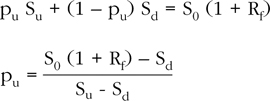
The stock price predicted by the cost of carry at the end of period 1 should be the average of S_u and S_d. This average is equal to the initial stock price, S₀, grossed up by the cost of carry to S₀ (1 + R_f)¹. Thus, it is necessary to solve for the weights or “probabilities” that equate the average of S_u and S_d to S₀ (1 + R_f)¹. Define p_u as the risk-neutral probability of obtaining S_u, and p_d as the risk-neutral probability of obtaining S_d at the end of the period. “Risk-neutral” in this context means that the average payoff may be discounted at the risk-free rate, which implies that investors act as if there is no need for a risk premium. Importantly, these are not the probabilities that the stock will go up or down. They measure the amount by which the stock may go up or down. These measures also adjust the future stock values so that they can be discounted at the risk-free rate. No direct probabilities of the stock going up or down are estimated. Subjective probabilities consequently are absent from the analysis. We refer to p_u and p_d as probabilities for convenience because they share the traditional characteristic of exhaustively summing up to 100%.⁶ Thus, p_u + p_d = 1, and, consequently, p_d = (1 – p_u). Solving for p_u:

Forming a Riskless Portfolio of Stock and Call Options

Chapter 1, “Arbitrage, Hedging, and the Law of One Price,” explains that, in the absence of any mispricing, a riskless portfolio should earn the risk-free rate. Consider a portfolio containing long stock and short-call options. Is there a mix of stock and options that provides a riskless, hedged position? If so, the price of the call that precludes arbitrage can be determined in the context of that riskless portfolio. Because the call option’s value is tied to that of the underlying stock, a riskless combination of both assets will contain offsetting elements—at least one long and one short.

Define the hedge ratio as the number of shares of long stock per call option, written (short) as h₀. You will see that this ratio is of great significance both in the pricing of options and in describing the behavior of their prices. The initial value of the portfolio is h₀ S₀ – C₀, which consists of h₀ shares of long stock per call option written. The cost of forming the portfolio increases with the purchase of additional shares of (long) stock and decreases with the sale of additional (short) calls. To be riskless, the payoffs associated with the stock moving to either S_u or S_d at the end of the period must be equal. In other words, the portfolio should grow only by the riskless rate of return over time. It is consequently unexposed to variations in the value of either the stock or the option, because an appropriately offsetting long/short mixture of the two has been adopted. What is lost on one position is offset by gains on the other.

The value of the portfolio at the end of the period is either (h₀ S_u – C_u) or (h₀ S_d – C_d), where C_u is the value of the call at the end of the period if S_u occurs, and C_d is the value of the call if S_d occurs. The value of the portfolio of calls and stock reflects the net effect of either an increase or decrease in the stock’s price. As noted, the payoffs at the end of the period must be equal for the portfolio to be riskless. Thus:

h₀ S_u – C_u = h₀ S_d – C_d

The hedge ratio consistent with a riskless portfolio is found by solving for h₀ in the preceding expression:

Consider the interpretation of h₀. The numerator measures the volatility of payoffs on the call option, and the denominator represents the volatility of the stock values at the end of the period. The hedge ratio thus balances changes in the value of the short calls against changes in the value of the long stock in an offsetting fashion that renders the portfolio riskless. Thus, one interpretation of the hedge ratio is as the mix of stock and call options that produces a riskless portfolio. You will soon see that the call must be priced in light of this capacity to generate a risk-free return when combined as described with the underlying stock, or an arbitrage opportunity will be created.

The hedge ratio may also be interpreted as the change in the value of calls per unit of change in the value of the underlying stock. Thus, h₀ = ΔC/ΔS. The ratio consequently measures the call option’s sensitivity to variations in the stock’s value. This is called the delta of a call option. Thus, the ratio serves double duty by describing the risk-free hedging mixture of long stock and short calls and by measuring how much call prices are expected to move in response to changes in the value of the underlying stock.⁷ As explained in detail in the next section, the value of delta must be between 0 and 1 for calls.

Pricing Call Options Using the Backward Induction Technique

It is necessary to determine the values of C_u and C_d at the end of the period to estimate the current value of the call option, C₀. The payoffs on the options are determinate because these are European options, and the current model considers only one period. In other words, there will be no speculative value, only intrinsic value at the end of the single period, which is the option’s expiration day.⁸ More concisely, C_u = max (0, S_u – X) and C_d = max (0, S_d – X), where X is the option’s exercise price. This means that the payoff on the call will be equal to the greater of 0 or the difference between the value of the stock on the expiration date and the exercise price. The payoff on the call cannot be negative, because the holder of a call option cannot be forced to exercise the option when it is not in his or her best interest. For example, consider the case in which S_u = $50, S_d = $40, and X = $45. Thus, C_u = max (0, $50 – $45) = $5 and C_d = max (0, $40 – $45) = 0. C_d cannot pay off –$5, because that would incorrectly imply that an investor would willingly exercise his or her right to buy the stock at $45 when it was worth only $40. Why buy a stock at an above-market price?

The time value of money suggests that the call’s current price should be the present value of the average payoff provided by the call option at the end of the period. Recall that we solved for the probabilities that weight C_u and C_d to provide an average expected payout equal to the forward price of the underlying stock price. This is tantamount to assuming that investors are risk-neutral and thus that the risk-free return is the appropriate discount rate. The current price of the call consequently is:

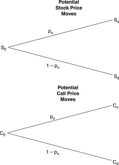
where p_u is defined as before and p_d = (1 – p_u). This expression takes the present value of the payoffs that can be generated by the call option at expiration. This is the so-called backward induction valuation technique, which determines the call option’s current value by first calculating the payoffs at the “backward” portion, or the expiration of the option’s life, and then uses the inductive method to infer its present value. The technique works because the payoffs on the option are known on its expiration date; it is either in, at, or out-of-the-money. The approach is especially helpful when multiple periods are involved. Figure 6.1 portrays the potential stock and call price moves over the single period under consideration.

Figure 6.1. One-Period Binomial Option Pricing Model Framework

Example of Applying the One-Period Binomial Option Pricing Model

Let’s calculate the current price of a European call on Yahoo, Inc. (YHOO) with an exercise price of $30.00. For illustrative purposes, assume that YHOO’s current price is $30.35, the risk-free rate is 3%, there is one period until expiration, and the stock price could go up by 20% (1 + u = 1.2) or down by 17% (1 + d = 0.83). Thus, S_u = $30.35 (1.20) = $36.42, and S_d = $30.35 (0.83) = $25.19. To apply the risk-neutral valuation method, we calculate the cost of carry price of YHOO in one period as:

S₀ (1 + R_f)¹ = $30.35 (1.03) = $31.26

As discussed, the risk-neutral probability p_u can be calculated so that the average payoff equals the cost of carry-based forward price:

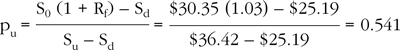
By implication, p_d = (1 – 0.541) = 0.459.

It is helpful to confirm that the risk-neutral probabilities produce an average future stock price equal to the cost of carry-based forward price of $31.26. The average is p_u S_u + p_d S_d = 0.541 (36.42) + 0.459 (25.19) ≈ $31.26. Thus, the risk-neutral probabilities achieve the desired goal, and the associated payoffs on the option can be discounted at the risk-free rate of return.

The current value of the call C₀ is based on the option payoffs at expiration, which are C_u = max (0, $36.42 – $30.00) = $6.42 and C_d = max (0, $25.19 – $30.00) = 0. Thus, the call’s current price is:

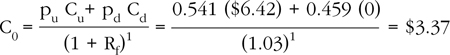
Demonstration That the Calculated Call Price Is Arbitrage-Free

If the preceding analysis is correct, the $3.37 call option price should preclude an arbitrage opportunity. In other words, if we adopt the appropriate hedge ratio when combining long YHOO stock and short YHOO call options at the indicated price of $3.37, the portfolio should generate the risk-free rate of return regardless of what happens to the stock price over the single period. The appropriate hedge ratio in this example is:

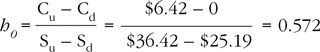
A hedged portfolio consequently is formed by buying 572 shares of YHOO and selling short 1,000 YHOO call options. The cost of the portfolio is h₀ S₀ – C₀ = 0.572 ($30.35) – $3.37 ≈ $13.99 per call written, which implies a total cost for 572 shares long and 1,000 short calls of $13,990.20.

As explained, if this portfolio is riskless, it should produce the same payoff no matter what happens to the price of YHOO, and the implied return should be the risk-free rate. Recall that the price of YHOO at the end of the period is either S_u = $36.42 or S_d = $25.19, and the associated future payoff of the call option is either C_u = $6.42 or C_d = 0. If YHOO moves up, the portfolio’s value consequently is 572 ($36.42) – 1,000 ($6.42) = $14,412.24. If YHOO moves down, the portfolio’s value is 572 ($25.19) – 1,000 (0) = $14,408.68. The portfolio values are the same but for modest rounding error.⁹ The implied returns are ($14,412.24/ $13,990.20) – 1 ≈ 3% and ($14,408.68/$13,990.20) – 1 ≈ 3%. Thus, regardless of what happens to YHOO’s price, the portfolio’s value is approximately the same, and the implied return is equal to the risk-free rate of 3%.

Exploiting an Arbitrage Opportunity in the One-Period Binomial Option Pricing Model

The appropriateness of the preceding call price of $3.37 is also confirmed by the arbitrage opportunity created by a deviation from that price. Consider prices that are significantly above and below the arbitrage-free price of $3.37. For example, what if the price of the call is $4.00 rather than the arbitrage-free price of $3.37? Common sense suggests that we sell the overvalued call and buy the underlying YHOO stock in the mixture dictated by the hedge ratio. Given a hedge ratio of 0.572, the arbitrage strategy is to buy 572 shares of YHOO and sell 1,000 calls. Let’s develop some intuition concerning the indicated arbitrage strategy.

The rate of return in this situation is expected to differ from the risk-free rate because the call price is too high. Indeed, the strategy’s rate of return should exceed the risk-free rate because the overvalued short calls generate too much money and thereby reduce the initial investment required to construct the portfolio. Yet the portfolio generates the same payoff at the end of the period as that in our prior analysis. In other words, the initial investment is lower while the payoff on the portfolio remains the same. Thus, the rate of return must increase.

In terms of our specific example, the revised initial investment is h₀ S₀ – C₀ = 0.572 ($30.35) – $4.00 ≈ $13.36 per call written, which implies a total cost for 572 shares long and 1,000 short calls of $13,360.20. The implied returns are ($14,412.24/$13,360.20) – 1 ≈ 7.87% and ($14,408.68/$13,360.20) – 1 ≈ 7.85%. Thus, the two outcomes again generate the same rate of return but for rounding error, and the returns are considerably in excess of the risk-free rate of return of only 3%. This should increase the investors’ desire to sell the options, thereby putting downward pressure on their price.

Alternatively, what if the price of the call option were too low, at a price of only $3.00? In this case, the arbitrage strategy is to buy the undervalued calls and hedge the position by selling short the underlying YHOO stock. This should be done consistent with the original hedge ratio calculated earlier so as to ensure the same riskless payoff at the expiration of the options. Thus, sell short 572 shares of YHOO at $30.35 and buy 1,000 call options at $3.00, which generates a net cash inflow of $3.00 (1,000) – 572 ($30.35) ≈ –$14,360.20. Because we have bought calls and sold short the stock, the payoffs at the option’s expiration are now net cash out-flows. The situation may be viewed as borrowing $14,360.20 and paying back $14,412.24 or $14,408.68. The implied borrowing rates are ($14,412.24/$14,360.20) – 1 ≈ 0.36% and ($14,408.68/ $14,360.20) – 1 ≈ 0.34%. Again, the two outcomes generate the same rate of return but for rounding error, and yet the implied borrowing rates are far below the 3% risk-free rate of return. It is obviously valuable to borrow below the risk-free rate. This should increase investors’ desire to buy the options, thereby putting upward pressure on prices.

In summary, the arbitrage-free call price of $3.37 is sustainable because significantly higher or lower prices create arbitrage opportunities that naturally push option prices back to that arbitrage-free level. Misvalued options are exploited by constructing a portfolio of stock and call options in the mixture dictated by the hedge ratio. In such strategies, the primary position is the option—long or short depending on whether it is undervalued or overvalued. The stock position is secondary in that it completes the risk-free hedge.

Two-Period Binomial Option Pricing Model

Description of the Framework and Rationale for Analysis

The one-period binomial model reveals the essential intuition of how arbitrage forms option prices. It is also necessary to explore how options are priced over multiple time periods. Multi-period applications of the binomial model still consider only two possible price moves at a time—up or down. Furthermore, multi-period models consider a time period to correspond to a price move. Thus, a period’s length is arbitrary. We explore the two-period model because it shows how the hedge ratio is revised over time so as to retain a riskless position no matter what happens to the price of the underlying stock.

Calculating the Price of a Call in the Two-Period Binomial Option Pricing Model

Our extension of the model to two periods uses the same data from the one-period model example. We consequently recalculate the current price of a European call on Yahoo, Inc. (YHOO) with an exercise price of $30.00, but now we consider potential price moves over two periods rather than just one. We continue to assume that the current price of YHOO is $30.35, that the risk-free rate is 3%, and that the stock price can go up by 20% (1 + u = 1.2) or down by 17% (1 + d) = 0.83) each period. It is important to keep in mind that the potential variability in the underlying stock price is the same for each period and that we consider moves over a total of two periods.

At the end of the first period, we still find S_u = $30.35 (1.20) = $36.42 and S_d = $30.35 (0.83) = $25.19. Due to our extension, there are now four possible future values of the stock at the end of period 2, only three of which are distinct. Specifically, over the two periods, the stock can go up at the end of the first period and then up again at the end of the second period, which leaves us at S_uu = S₀ (1+ u) (1+ u) = S₀ (1+ u)² = $30.35 (1.20)² = $43.70. If the price goes up the first period and then down, the price at the end of period 2 will be S_ud = S₀ (1+ u) (1+ d) = $30.35 (1.20)(0.83) = $30.23. If the price goes down first and then up, the price at end of period 2 will be S_du = S₀ (1+ d) (1+ u) = $30.35 (0.83)(1.20) = $30.23. Finally, if the price of YHOO goes down each period, the price at the end of period 2 will be S_dd = S₀ (1+ d) (1+ d) = $30.35 (0.83)² = $20.91.

Notice that with constant percentage periodic potential moves of u and d, S_ud = S_du = $30.23. Thus, there are only three different prices at the end of the second period. This is called a recombining price tree because the same price can result independent of how you got there over multiple periods of time. In other words, you end up with a price of $30.23 regardless of whether the price first went up and then down or whether it went down first and then up.

The backward induction valuation technique is applied to calculate the option’s current value in the two-period model. The value of the call at the end of period 1 cannot be captured through exercise at that time because this is a European option, which can be exercised only at expiration. The values of the call at the end of period 1 should nonetheless reflect the potential payoffs available through the exercise of the call at its expiration at the end of period 2. Consequently, the option’s current value should depend on the payoffs available on the expiration date through exercise. Because we cannot exercise the call at the end of the first period, the values at that time may be viewed as “placeholders” that reflect the value of the payoffs at the end of period 2. Thus, we see the application of the backward induction valuation approach.

The payoffs at the end of period 2—the payoffs at the “back” of the option’s life—can be used to infer the call’s values at the end of the first period. In turn, these can be used to infer the call’s current value. Two-period valuation can be seen as the culmination of a two-step valuation process in which we move backward from the expiration date to the current time in a period-by-period sequence.¹⁰

Let’s use the preceding information to calculate the current price of a European call on YHOO under the two-period framework. We compute the call’s price by applying the previously developed binomial approach on a period-by-period basis. The one-period model computes C₀ as the present value of the weighted average of C_u and C_d, in which the weights are the risk-neutral probabilities that the stock will go up (p_u) versus down (p_d). We use the same approach while recognizing that C_u and C_d should reflect the values of the payoffs on the option at the end of period 2. Specifically, C_u should capture the payoffs associated with C_uu and C_ud in the same fashion that C₀ reflects the payoffs associated with C_u and C_d at the end of period 1 in the one-period model. Similarly, C_d should capture the payoffs associated with C_du and C_dd as C₀ reflects the payoffs associated with C_u and C_d at the end of period 1. Consequently, this valuation approach determines the call’s current value by applying the one-period binomial option pricing model twice in sequence.

Recall that the call option has an exercise price of $30.00, the risk-free rate per period is 3%, the current stock price is $30.35, and the stock price could go up by 20% (1 + u = 1.2) or down by 17% (1 + d = 0.83). Thus, S_u = $36.42, S_d = $25.19, S_uu = $43.70, S_ud = S_du = $30.23, and S_dd = $20.91. Furthermore, recall that p_u = 0.541 and p_d = (1 – p_u) = 0.459. To calculate the current value of the call C₀, we first calculate the value of the option payoffs at the end of period 2 as of the end of period 1. It is clear that C_u depends on C_uu and C_ud. These payoffs are calculated as C_uu = max (0, S_uu – X) = max (0, $43.70 – $30.00) = $13.70 and C_ud = max (S_ud – X) = max (0, $30.23 – $30.00) = 0.23. Similarly, C_d depends on C_du and C_dd. These payoffs are calculated as C_du = max (S_ud – X) = max (0, $30.23 – $30.00) = 0.23 and C_dd = max (S_dd – X) = max (0, $20.91 – $30.00) = 0. Each of the two option values, C_u and C_d, is the present value of the associated average payoff at the end of period 2 as of the end of period 1. The values of the call at the end of period 1 are thus:

and

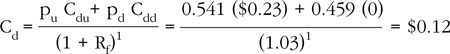
Continuing the backward induction process, we determine the appropriate current price of the call option C₀ as the present value of the average value of the option at the end of period 1:

Notice that this two-period price exceeds the previously calculated one-period price of $3.37. This appeals to our intuition that, everything else being equal, a longer-term option should be worth more than a shorter-term option.

Calculating and Interpreting Hedge Ratios in the Two-Period Model

While the stock prices at the end of period 1 are the same under both the one- and two-period models, the hedge ratio h₀ that renders the long stock/short call portfolio riskless changes over the two periods. This is because the values of C_u and C_d differ from their one-period values now that there is an additional time period until expiration. Consequently, there is no reason to expect the hedge ratio to remain the same as in the one-period model or to be the same over both time periods in the two-period model.

At the beginning of the first period, we do not know what the stock price will be at the end of that period, much less where the price will be at the end of the second period. This is why we adopt the hedge ratio that ensures the same portfolio value at the end of the first period regardless of where the price ends up. However, at the end of the first period, some uncertainty is resolved because we know then whether the price went up or down. Importantly, this should change the hedge ratio, because knowing where the stock price is at the end of the first period reduces the range of possible payoffs faced by the investor at the end of period 2. Thus, when the risk of the payoffs changes, the hedge ratio that protects against that risk should also change. As explained earlier, this is the key insight provided by the two-period model: changes in the underlying stock’s price bring changes in the ratio necessary to hedge a portfolio of long stock and short calls.

A change in the risk-neutralizing hedge over time implies that the price of a one-period call differs from that of a two-period call because the cost of the replicating portfolio changes. This finding is significant. For example, as the number of periods increases to accommodate a more extensive set of potential price moves, the frequency with which a portfolio must be rebalanced to remain riskless increases. In the continuous-time context of the Black-Scholes-Merton option pricing model, a portfolio of long stock/short calls must be rebalanced continuously to remain riskless. Given that portfolio rebalancing is costly, this implies that the benefits of rebalancing must be weighed carefully against its costs.

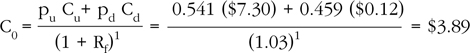
Figure 6.2 shows the details of hedging and pricing options periodically in a two-period context. The hedge ratio that protects the portfolio over the first period is:

Figure 6.2. Two-Period Binomial Option Pricing Model Framework

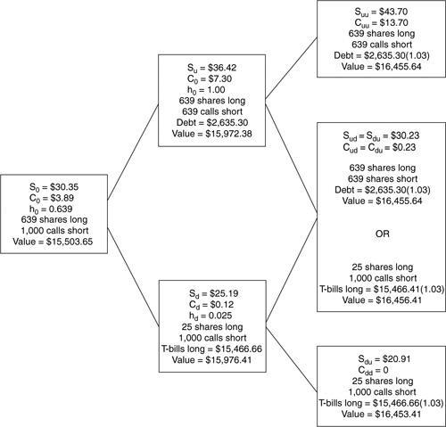
Thus, a hedged portfolio is formed by buying 639 shares of YHOO and selling short 1,000 YHOO call options. Recall that the hedge ratio in the one-period model was 0.572. The initial hedge ratio in the two-period model exceeds that in the one-period model because of the greater range of possible future stock prices at expiration. Thus, it takes more shares of stock to protect the short call position in light of the greater risk posed by the additional share price variability in a two-period context.

At the end of period 1, two possible hedge ratios exist: h_u, which is associated with the price going up to S_u, and h_d, which is associated with the price going down to S_d. Two different hedge ratios exist because the risk over the remaining period differs according to whether the stock price goes up or down at the end of the first period. Thus, different long stock/short call mixtures are needed to ensure that the portfolio remains riskless over the second period.

We rely on the stock prices and previously calculated payoffs as of the end of period 2 to calculate the hedge ratios at the end of the first period: S_uu = $43.70, S_ud = S_du = $30.23, S_dd = $20.91, C_uu = $13.70, C_ud = C_du = $0.23, and C_dd = $0. Extending the prior approach, the two hedge ratios are:

and

One of the most important insights of the two-period binomial model emerges from interpreting these hedge ratios. This helps us develop more economic intuition about arbitrage in general and option pricing in particular. As noted, the initial hedge ratio was 0.639. When the stock price moves up at the end of the period, the hedge ratio increases to h_u = 1.00. Conversely, when the stock price moves down at the end of the period, the hedge ratio decreases to h_d = 0.025.

Consider why these hedge ratio changes make sense. Recall that each hedge ratio measures how many shares of stock must be held per call written to maintain a riskless position over the subsequent period. Furthermore, each also measures the expected responsiveness of call prices to changes in the price of the underlying stock. The connection between these two interpretations is that the relative sensitivity of call prices to stock price moves dictates the specific mixture of the two assets that creates a riskless portfolio. Either interpretation implies that such hedge ratios should have an absolute value between 0 and 1. Thus, the call and stock price are less related when the option is out-of-the-money, more highly related when the option is in-the-money, and somewhat related when an option can end up in or out-of-the-money at the end of the given period.

Let’s apply these observations concerning the intuition behind the magnitude of the hedge ratio to the preceding data. Visualize being at the end of period 1 in Figure 6.2. If you are at the upper node, the option will definitely finish in-the-money, and the hedge ratio is 1. This means that it is necessary to hold one share of stock for every call written to cover the risk associated with the cash payout on the in-the-money short call options at expiration.

The call option is expected to mirror stock price moves one-forone because the option is in-the-money. If you are at the lower node, the option may or may not end up in-the-money. If it does end in-the-money, it will be only modestly so. Thus, the hedge ratio is closer to 0 than to 1. It is consequently necessary to hold little stock to cover the payout on the short call option. The call option is expected to capture only a small amount of any move in the underlying stock’s price, because only one of the possible stock prices pushes the call in-the-money by a small amount while the other leaves the option out-of-the-money. If the subsequent outcomes were all out-of-the-money at a node, the hedge ratio would be 0. This provides some intuition concerning why the two ratios move as they do in response to the stock price’s going up or down at the end of the first period.

Portfolio Rebalancing Over Time

The portfolio of long stock/short calls must be rebalanced at the end of the first period if it is to remain riskless over the second period. One “size” (hedge ratio) does not “fit all” (both periods). Continuing the preceding example, we show how the portfolio is rebalanced periodically and explain that this process implies that the calculated call price of $3.89 should preclude an arbitrage opportunity. In other words, if we adopt the appropriate initial hedge ratio, the portfolio should generate the risk-free rate of return regardless of what happens to the stock price over the first period. The portfolio should also generate the risk-free return over the second period if it is rebalanced to conform to the new hedge ratio revealed at the end of the first period in light of what could happen to the stock price over the second period. The organizing principle is important enough to restate: A portfolio remains hedged only if it is rebalanced, and a hedged portfolio involving correctly priced assets should earn the risk-free rate of return.

Recall that the initial hedge ratio is 0.639 and that the hedge ratios in effect at the end of the first period are h_u = 1.00 if the price increases and h_d = 0.025 if the price falls. A portfolio consequently is hedged over the first period by buying 639 shares of YHOO and selling short 1,000 YHOO call options. The cost of establishing the portfolio is h₀ S₀ – C₀ = 0.639 ($30.35) – $3.89 ≈ $15.50 per call written, which implies a total cost for 639 shares long and 1,000 short calls of $15,503.65.

Let’s confirm that adopting the initial hedge ratio h₀ produces the same payoff at the end of the first period no matter what happens to the price of YHOO. It is also important to confirm that the implied return equals the risk-free rate. Recall that the price of YHOO at the end of the period can move to either S_u = $36.42 or S_d = $25.19 and that the associated values of the call option are either C_u = $7.30 or C_d = $0.12. If YHOO increases, the value of the portfolio is consequently 639 ($36.42) – 1,000 ($7.30) = $15,972.38. If YHOO decreases, the value of the portfolio is 639 ($25.19) – 1,000 ($0.12) = $15,976.41. The portfolio values are roughly the same but for rounding error.¹¹ The implied returns are ($15,972.38/$15,503.65) – 1 ≈ 3% and ($15,976.41/$15,503.65) – 1 ≈ 3%. Thus, regardless of what happens to YHOO’s price, the values of the portfolio at the end of the first period are approximately the same, and the implied returns are equal to the risk-free rate. This implies that the calculated call price of $3.89 is arbitrage-free.

At the end of the first period, we know whether the price went up or down, which resolves some of the uncertainty concerning where the price will end up at the end of the second period. At the end of period 1, we consequently adopt the hedge ratio that captures the new range of prices that will prevail at the end of period 2. Consider how the portfolio should be rebalanced if the stock price increases to S_u = $36.42 at the end of the first period. In that case, the portfolio should be rebalanced to conform to the new hedge ratio of h_u = 1.00. Thus, the portfolio needs to move from a hedge ratio of h₀ = 0.639 to h_u = 1.00, which implies that the ratio of stocks held long-to-short calls written needs to move to a 1:1 ratio. There are two ways to effect such a change: increase the number of shares held from 639 to 1,000 to match the 1,000 short calls, or decrease the number of short calls held from 1,000 to 639. An investor would presumably choose the cheaper of the two approaches. However, choosing the cheaper of the two options only means that the investor will then have less invested. Regardless of the choice, the investor will earn the riskless rate of return on whatever remains invested in the hedged portfolio. It is cheaper to buy back 361 options at C_u = $7.30 each for a total cost of $2,635.30 than to buy an additional 361 shares of stock at S_u = $36.42 each for a total cost of $13,147.62.

We assume that the investor rebalances by either borrowing needed funds or by investing funds generated by rebalancing—both at the risk-free rate. In this case, the investor borrows the $2,635.30 needed to buy back 361 call options at the 3% risk-free rate. The rebalanced portfolio consists of 639 shares of YHOO valued at $36.42, 639 call options valued at $7.30 each, and debt of $2,635.30. Thus, the portfolio’s net value is (639)($36.42) – (639)($7.30) – $2,635.30 = $15,972.38. This is, of course, about the same value of the portfolio at the end of period 1 that we previously calculated. However, that value has been reallocated across the stock, call options, and debt to be consistent with the new hedge ratio h_u. Notice as well that the portfolio rebalancing is self-financing. We show next that this rebalanced portfolio earns the risk-free return over the second period.

Now consider how the portfolio should be rebalanced if the stock price decreases to S_d = $25.19 at the end of the first period. In this case, the portfolio should be revised from a hedge ratio of h₀ = 0.639 to h_d = 0.025, which implies that very few shares of stock need be held to protect the 1,000 short calls. Indeed, only (0.025)(1,000) = 25 shares are needed. Thus, the investor should sell 639 – 25 = 614 shares. Given how close the option is to being out-of-the-money, we expect it to exhibit little sensitivity to changes in the price of the underlying stock. Given that S_d = $25.19, this stock sale generates (614)($25.19) = $15,466.66 in cash, which will be invested over the second period at the 3% risk-free rate of return. The rebalanced portfolio consequently consists of 25 shares of YHOO valued at $25.19, 1,000 short call options valued at $0.12 each, and a Treasury bill investment of $15,466.66. Thus, the portfolio’s net value is (25)($25.19) – (1,000)($0.12) + $15,466.66 = $15,976.41. Once again, this is about the same value as that of the portfolio at the end of the period. As in the prior case, the portfolio rebalancing is self-financing. We have just reallocated that value across the stock, call options, and T-bill investment to meet the requirements of the new hedge ratio h_d. We show next that this rebalanced portfolio earns the risk-free return over the second period.

The values of the portfolio at the end of period 2 should be the same regardless of what happens to the price of YHOO if the hedge ratios provide the desired risk protection. First consider the values of the portfolio at the end of the second period if the price went up at the end of the first period. In other words, what are the values of the hedged portfolio if either S_uu = $43.70 or S_ud = $30.23 is obtained at the end of period 2 and we had adopted the indicated hedge ratio h_u at the end of period 1?

If YHOO’s price goes to S_uu = $43.70, the associated call price is C_uu = $13.70. Given that the hedge ratio h_u = 1.00, we previously noted that the rebalanced portfolio contains 639 shares of YHOO, 639 short call options, and debt of $2,635.30. The debt must be paid off with 3% interest at the end of period 2. Thus, the net value of the portfolio under this scenario at the end of period 2 is (639)($43.70) – (639)($13.70) – $2,635.30 (1.03) = $16,455.64. Recall that the value of the portfolio at the end of period 1 associated with a price increase was $15,982.38. Thus, in this situation the return on the portfolio over the second period is ($16,455.64/ $15,972.38) – 1 ≈ 3%.

The other branch of the binomial tree emanating from an increase in the price at the end of period 1 takes us to a price of S_ud = $30.23 and an associated call price of C_ud = $0.23 at the end of the second period. Again, assuming that we adopted the appropriate hedge ratio h_u = 1.00 at the end of period 1, the rebalanced portfolio still consists of 639 shares of YHOO, 639 short call options, and debt of $2,635.30. As noted, the debt must be paid off with 3% interest at the end of period 2. The net value of the portfolio under this scenario at the end of period 2 thus is (639)($30.23) – (639)($0.23) – $2,635.30 (1.03) = $16,455.64. Given that the value of the portfolio at the end of period 1 associated with a price increase was $15,972.38, this implies that the return on the portfolio over the second period is ($16,455.64/$15,972.38) – 1 ≈ 3%. Thus, after the price of YHOO goes up at the end of period 1, a portfolio hedged at h_u has the same value at the end of the second period whether the price goes up or down from that point. Thus, the hedge ratio of h_u = 1.00 has provided the desired protection.

Now, consider the values of the portfolio at the end of the second period if the price goes down at the end of the first period. In other words, what are the values of the hedged portfolio if either S_du = $30.23 or S_dd = $20.91 occurs at the end of period 2 and we had adopted the indicated hedge ratio of h_d = 0.025 at the end of period 1? If YHOO’s price goes to S_du = $30.23, the associated call price is C_du = $0.23. Given the hedge ratio of h_d = 0.025, we previously noted that the rebalanced portfolio consisted of 25 shares of YHOO, 1,000 short call options, and a T-bill investment of $15,466.66, which had a total value of $15,976.41. The Treasury bill investment will return the principal plus 3% interest at the end of period 2. Thus, the net value of the portfolio at the end of period 2 is (25)($30.23) – (1,000)($0.23) + $15,466.66 (1.03) = $16,456.41. Recall that the value of the portfolio at the end of period 1 associated with a price decrease was $15,976.41. Thus, the return on the portfolio over the second period is ($16,456.41/ $15,976.41) – 1 ≈ 3%.

On the other hand, a decrease in the price at the end of period 1 could also end up at a price of S_dd = $20.91 at the end of period 2, which implies an associated call price of C_dd = $0. Again assuming that we adopted the appropriate hedge ratio of h_d = 0.025 at the end of period 1, the rebalanced portfolio consisted of 25 shares of YHOO, 1,000 short call options, and a Treasury bill investment of $15,466.66. As noted, the T-bill investment will return the principal plus 3% interest at the end of period 2.

The net value of the portfolio is (25)($20.91) – (1,000)($0) + $15,466.66 (1.03) = $16,453.41. Given that the value of the portfolio at the end of period 1 associated with a price decrease was $15,976.41, this implies that the return on the portfolio over the second period is ($16,453.41/$15,976.41) – 1 ≈ 3%. Thus, after the price of YHOO goes down at the end of period 1, a portfolio hedged at h_d has about the same value at the end of the second period no matter whether the price goes up or down from that point. Again, the hedge ratio has provided the desired protection.

This analysis shows that the portfolio will earn the risk-free return each period if it is rebalanced each period to conform to the applicable hedge ratio. In the two-period case, this means that if we adopt h₀ initially and then rebalance the portfolio at the end of period 1 to h_d if S_d has occurred or to h_u if S_u has occurred, the portfolio will earn the risk-free return in both periods 1 and 2.

For completeness, let’s confirm that the two-period rate of return is equal to the risk-free rate of return. Of course, we expect this result because the two sequential one-period returns are equal to the risk-free rate. Recall that the initial portfolio dictated by h₀ = 0.639 has a total value of $15,503.65. If YHOO moves up to S_uu = $43.70 at the end of period 2, the portfolio’s value is $16,455.64. Alternatively, if the price of YHOO moves to S_ud = S_du = $30.23, the portfolio’s value is $16,455.64 or $16,456.41. Finally, if YHOO’s price falls to S_dd = $20.91, the portfolio’s value is $16,453.41. Thus, but for minor rounding error, the value of the hedged portfolio is the same across all potential values of the stock and its associated call option at the end of period 2.

For simplicity, let’s use the average of these possible portfolio values at the end of period 2 of $16,455.28 to calculate the two-period return. Given a value at the beginning of the two-period horizon of $15,503.65, the return is calculated as ($16,455.28/ $15,503.65)^1/2 – 1 ≈ 3%. This confirms our expectation that the two-period return equals the risk-free rate and thus that the periodic rebalancing strategy does indeed protect the portfolio over the entire time horizon.

The Black-Scholes-Merton Option Pricing Model

The binomial option pricing model presented here provides intuitive insight into how arbitrage determines option prices. As discussed, the Nobel Prize was awarded for developing the so-called Black-Scholes-Merton (BSM) option pricing model, which predates the binomial approach. Although the derivation and extensive exploration of the BSM approach is beyond the scope of this book, it is important to briefly consider how the model relates to the binomial approach to reinforce our understanding of arbitrage in this context.

The binomial option pricing approach considers discrete time periods that portray only two possible future stock prices for each future period. We expect the binomial approach to more accurately capture reality as the number of periods increases, which implies that the length of the implicit time periods decreases. Thus, enter the BSM approach, which uses continuous time to portray a myriad of future stock prices measured using a probability distribution. A primary value of the BSM model is to broaden the range of future stock prices reflected in pricing an option by using infinitesimally short time periods.

As in the binomial approach, the BSM model relies on a self-financing, riskless arbitrage strategy that replicates the cash flow profile of a European call option on a stock that pays no dividends. The BSM approach relies on the appropriate combination of the underlying stock and borrowing at a given time that replicates that cash flow pattern of the call option. Thus, the price of a call option estimated by the BSM model satisfies the arbitrage-free conditions identified in the context of binomial pricing. Obviously, a stock’s price can change from instant to instant during a trading day. This implies that the combination of stock and borrowing required to replicate a call option can also change from instant to instant. Thus, practical application of the BSM model to hedging situations must balance the costs and benefits of rebalancing a hedge in light of transactions costs.

The formula used to price call options under the BSM model is:

C₀ = S₀ N (d₁) – Xe^{–R_c(T – t)} N (d₂)

where

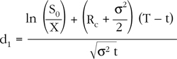
and

The following variables have not been defined yet:

• T is the expiration date, and t is the time at which the option is priced—both stated as a percentage of a year.

• e is Euler’s 2.1718.

• R_c is the annualized continuous-time risk-free rate.

• N(d_i) is the probability that a standardized random variable that is normally distributed will be less than or equal to d (i = 1 or 2).

• ln is the natural log of the given quantity.

• σ² is the annualized variance of the continuous return on the stock.

The BSM makes numerous technical assumptions:

• It applies only to European options.

• There are no transactions costs or taxes.

• There are no restrictions on short selling.

• The stock price follows a lognormal probability distribution.

• The stock price moves continuously without jumps.

• The interest rate is constant.

• The stock does not pay dividends.

Although these assumptions seem quite restrictive, accommodations can be made to handle their violation. Indeed, evidence shows that the BSM model produces reasonably accurate call option prices.

For our purposes, it is sufficient to observe that the BSM equation relies on the same general determinants of option value revealed in the binomial option pricing approach. Thus, European call option prices estimated using the BSM model are determined by the stock price, the option’s exercise price, the volatility of future stock prices, the risk-free interest, and the time to expiration. Consistent with the binomial option pricing approach, the BSM model also presents a call option’s price as the cost of constructing a risk-free hedged portfolio that replicates that option’s payoff structure. Importantly, option pricing does not rely on the expected return on the underlying asset.

Summary

This chapter explained how arbitrage forms the backbone of modern option pricing. After considering the binomial option pricing model presented in this chapter, perhaps you may now occasionally think of option prices when you see fruit salad. Just like you can estimate the price of fruit salad by averaging the prices of the individual fruit in the salad, the model shows that an option can be valued by averaging the prices of its underlying components. The price of a call option depends on the underlying stock price, the time to expiration, the exercise price, the risk-free rate of return, and the volatility of the underlying stock. The “recipe” described by the hedge ratio forms a portfolio that replicates the cash flows of a call option. Specifically, it describes the mixture of stock and call options that is riskless over the life of the associated option. The appropriate arbitrage-free price of a call option is really just the cost of constructing a risk-free hedged portfolio that replicates the payoff structure of the option itself. Although an option’s payoff is not risk-free, arbitrage-free option prices are dictated by the cost of such a hedging strategy.

The one-period binomial model reveals the essential intuition of how arbitrage forms option prices. We used the two-period model to show how the portfolio should be revised over time so as to remain riskless no matter what happens to the price of the underlying stock. It is necessary to rebalance a portfolio periodically if it is to remain riskless.

Useful economic intuition about arbitrage in general and option pricing in particular can be obtained by interpreting hedge ratios. First, hedge ratios measure how many shares of stock must be held per call written to maintain a riskless position over a given investment horizon. Second, hedge ratios also measure the expected responsiveness of call prices to changes in the price of the underlying stock. The connection between these two interpretations of the hedge ratio is that the sensitivity of call prices to stock price moves dictates the specific mixture of the two assets that creates a riskless portfolio. Thus, call and stock prices generally are unrelated when the option is out-of-the-money, perfectly related when the option is in-the-money, and somewhat related when an option can end up in or out-of-the-money over the remaining time to expiration. This provides some intuition concerning why the two ratios move as they do in response to stock price movements. It also helps us understand the implied changes in the mixture of stocks and calls that maintains a riskless position over the investment time horizon.

The binomial option pricing model elegantly shows how the engine of arbitrage forms option prices in light of the ability to construct riskless, hedged portfolios that can replicate option payoffs. In a multi-period context this implies that an investor can earn the risk-free rate each period if he or she is willing to rebalance the portfolio each period to conform to the appropriate hedge ratio.

The chapter concluded by explaining how the Black-Scholes-Merton (BSM) option pricing model relates to the binomial option pricing approach. Whereas the binomial option pricing approach considers discrete time periods in which only two potential future stock prices are considered at a time, the BSM approach considers continuous time periods to portray a probability distribution of future stock prices. Thus, a major contribution of the BSM model is to broaden the range of future stock prices reflected in pricing an option.

The binomial and BSM option pricing approaches both rely on a self-financing, riskless arbitrage strategy that replicates the cash flow profile of a European call option on a stock that pays no dividends. Thus, the price of a call option estimated by the BSM model satisfies the arbitrage-free conditions identified in binomial pricing. Both modeling approaches consider the following to determine call option prices: the stock price, the option’s exercise price, the volatility of future stock prices, the risk-free interest rate, and the time to expiration. Furthermore, both approaches view a call option price as the cost of constructing a risk-free hedged portfolio that replicates the option’s payoff structure.

Endnotes

¹ My Life as a Quant (2004, p. 213).

² Myron Scholes and Robert Merton were awarded the Nobel Prize in Economic Sciences for their contributions to option pricing theory. Fisher Black’s contribution was cited by the Committee but, unfortunately, he had passed away, and the Prize is not awarded posthumously. The papers that were the basis for the Nobel Prize are Black and Scholes (1973) and Merton (1973).

³ See Cox, Ross, and Rubinstein (1979) and Rendleman and Bartter (1979).

⁴ Sources: Dunbar (2000), Edwards (1999), Lowenstein (2000), and Marthinsen (2005, Chapter 8).

⁵ More advanced analysis considers that many investors expect volatility to be different at different stock prices.

⁶ For these reasons, p_u and p_d are sometimes called “pseudo-probabilities” in the literature, which is accurate but a bit unwieldy.

⁷ It is important to note the technical qualification that delta is only an accurate measure of the price sensitivity of a call option for small changes in the price of the underlying stock. This is because the call price response is not linear across the entire range of the underlying stock’s price.

⁸ Intrinsic value is the extent to which S > X, which expresses the value of exercising a call option. Intrinsic value cannot be negative. Speculative value is the part of an option’s premium that exceeds intrinsic value. It measures how much is paid for the possible movement of the call either “in-the-money” or further “in-the-money” if it already has positive intrinsic value.

⁹ If a more precise estimate of the hedge ratio, such as 0.571708447, is used, the portfolio values are closer together: $14,401.62 vs. $14,401.34. The less precise estimate of 0.572 is used because fractional shares cannot be traded.

¹⁰ Alternatively, the call’s current value can be inferred directly from the potential payoffs at the end of the second period. This may be expressed in an algebraically equivalent formula that we do not develop because it relies on the same economic intuition as the preceding analysis.

¹¹ Again, the values of the two portfolios would be the same if a more precise hedge ratio was used. As before, the less precise estimate is used in light of our ability to trade only a discrete number of securities.