Chapter 5. Put-Call Parity and Arbitrage

It’s a wrong perception to believe that you can eliminate risk just because you can measure it.

—Professor Robert C. Merton, Nobel Laureate in Economic Sciences, 1997¹

Put-call parity describes the relationship among the values of put and call options on the same stock and a riskless security such as a Treasury bill (T-bill).² Specifically, the call price, put price, stock price, time to expiration, exercise price, and risk-free rate are related to one another systematically. Focusing on European options, we first demonstrate how the put-call parity relation holds. Then we show how to exploit deviations from the predicted relationship using arbitrage strategies. Next we explain how the relation can be used to create synthetic securities. Finally, put-call parity is used to examine some basic option/stock combination strategies.

The Put-Call Parity Relationship

Put-call parity can be demonstrated using the same framework presented in the arbitrage examples in Chapter 2, “Arbitrage in Action.” Recall that we examined the relationship between the prices of two stocks now and their respective values in two future possible outcomes. Our goal was to identify whether they offered equivalent future outcomes in some combination. We use the same general approach to establish the relationship among the values of puts and calls on the same stock and a riskless security in this chapter. We first explain the relationship generally and then reinforce the concept using market price data.

Consider a European call option with a price of C and a European put option with a price of P, both on the same underlying stock with a current price of S₀. For simplicity, we consider only a non-dividend paying stock. Furthermore, assume that the options have the same exercise price X and the same expiration date T and that U.S. Treasury bills maturing at the same time the options expire yield R_f percent. We also assume discrete rather than continuous compounding because it makes the presentation more intuitive. S_T is the value of the stock on the expiration date. Market data are used in an example after presenting the put-call parity relation.

Table 5.1 shows two portfolios containing the described securities. Portfolio A consists of a long stock and a long put. Portfolio B consists of a long call and a long T-bill with a face value of X maturing at the same time the options expire. Compare the values of the portfolios now and on the expiration date to reveal the relationship among the securities. The values of the respective portfolios are determinate on the expiration date because the options are worth only their intrinsic values at that time, and the T-bill matures to its face value.³

Table 5.1. Put-Call Parity for European Options

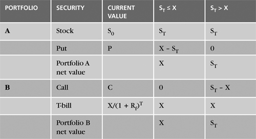
Before drawing key conclusions, let’s carefully explore Table 5.1. The initial investment in Portfolio A is S₀ + P, which is the sum of the prices of the long stock and the long put. The initial investment in Portfolio B is C + X/(1 + R_f)^T, which is the sum of the prices of the long call and the long T-bill. In Portfolio B, the second component can be viewed as the present value of the exercise price X or as the present value of the face amount X of the T-bill that will be paid at maturity. In searching for some intuition, think of the T-bill being in Portfolio B for two reasons: At maturity it provides the funds to pay the price needed to exercise a valuable call at expiration, and it introduces the risk-free rate of return into the analysis.⁴ Although we do not yet know the relationship between the current values of the two portfolios, it can be inferred on the basis of the relationship between the values of the two portfolios at expiration.

Table 5.1 shows the values of the two portfolios on the expiration date, assuming that the value of the stock is either less than or equal to the exercise price or greater than the exercise price. We examine these two outcomes because they express the two possible sets of cash flows generated by the option positions at expiration. The indicated net values relate the payoffs on each component to the respective overall portfolio.

Observe that Portfolio A’s net value is either X or S_T. Interestingly, on the expiration date, Portfolio B’s net value is the same as Portfolio A’s: X or S_T. Thus, if the two portfolios have the same payoffs at expiration, they should have the same current values as well. Put-call parity asserts that a portfolio of a stock and a put is equivalent to a portfolio of a call and a T-bill and therefore should be priced the same. This is consistent with our observation in Chapters 1 and 2 that equivalent combinations of securities should sell for equivalent prices. Equivalence in this context is the equality of payoffs at expiration.

In light of this observation, we can state put-call parity for European options as:

S₀ + P = C + X/(1 + R_f)^T

Put-call parity thus portrays the relationship among call and put prices, the underlying stock price, the exercise price, the risk-free rate, and the time to expiration.

Let’s look at data on Yahoo, Inc. (YHOO), the U.S. Internet company, to make our analysis more concrete. On July 12, YHOO was selling at $30.35. The August call with an exercise price of $30.00 was selling for $1.80, and the August put with an exercise price of $30.00 was selling for $1.41. The risk-free rate for the T-bill maturing closest to the options’ expiration was 1.29%. The time to expiration stated as a percentage of the year was 0.1096 (40/365). Put-call parity indicates that:

S₀ + P = C + X/(1 + R_f)^T

30.35 + 1.41 = 1.80 + 30.00/(1.0129)^0.1096

$31.76 ≈ $31.76

Thus, put-call parity holds.

Why Should Put-Call Parity Hold?

Put-call parity should hold because deviations create arbitrage opportunities that can be exploited, thereby returning the prices to no-arbitrage, steady-state values. Reconsider the YHOO data. Rather than the stock and put portfolio being priced at $31.76, assume that it is priced at $34.76. Thus, the stock and put portfolio is overvalued by $3.00. Although it is unnecessary to know whether the mispricing results from the stock or the put, we assume that the put is the source. Selling short the stock and put portfolio generates $34.76, whereas purchasing the call/T-bill portfolio costs only $31.76. Thus, the net result is an initial inflow of $3.00, which never has to be returned because the two portfolios cancel to a net value of zero at expiration. Let’s explore in detail how the arbitrage strategy should be implemented using the put-call parity framework.

As discussed, the stock/put portfolio is overvalued relative to the call/T-bill portfolio. We consequently sell short the stock/put portfolio and hedge that investment by buying the call/T-bill portfolio. The proceeds of the short sale exceed the cost of hedging the position with the long call/T-bill portfolio. Thus, the strategy generates an initial cash inflow of $34.36 – $31.36 = $3.00, which meets the self-financing requirement of arbitrage. While selling short the stock/put portfolio makes sense given its apparent mispricing, doing so alone would be risky. The strategy must also be demonstrably riskless.

Consider the arbitrage strategy shown in Table 5.2. Observe that the portfolio’s net value is initially –$3.00 because S₀ + P > C + X/(1 + R_f)^T, or $34.75 > $31.76. The interpretation of the negative initial investment is that the short sale of the stock/put portfolio generates more funds than it costs to go long the call/T-bill portfolio. This confirms that the strategy is self-financing. Also note that both of the portfolios’ net payoffs at expiration are zero. This makes sense, because the stock/put and call/T-bill portfolios ultimately generate the same payoffs at expiration, which cancel each other out because one position is long (call and T-bill) and the other is short (stock and put). This means that the strategy is riskless. This outcome is provocative: The arbitrage strategy generates money upfront that never has to be given back! This is like receiving a loan that the bank never requires to be paid back. Thus, put-call parity should hold because significant departures can be exploited in this fashion.

Table 5.2. Arbitrage Strategy Using Put-Call Parity: Overvalued Stock/Put Portfolio

The put-call parity expression may be rearranged algebraically to identify a variety of identical portfolios that should be priced consistently. For example, solving for the value of the call in the put-call parity expression yields the following:

C = S₀ + P – X/(1 + R_f)^T

Thus, a call is equivalent to a portfolio of a long stock, long put, and short T-bill. Note that selling short a T-bill is equivalent to borrowing at the risk-free rate.

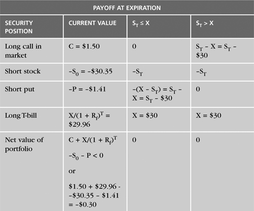
In terms of our data, let’s assume that the call is priced at $1.50 instead of the appropriate $1.80. Clearly, we would like to buy the call, because it is undervalued by $0.30. However, we prefer to exploit the misvaluation using an arbitrage strategy that is, by definition, self-financing and riskless. The strategy may be rendered riskless by hedging the long call with a position that is equivalent to a properly priced short call. Such a joint position would risklessly lock in the difference between the undervalued call and the correctly-valued position that is equivalent to the call. In other words, the arbitrage portfolio is effectively long a real call and short a synthetic call. The combined positions cancel out all risk.

Let’s develop some intuition concerning the construction of the arbitrage portfolio by applying a simple rule. In terms of the put-call parity relation restated to isolate the call, we buy the “left side” (the call trading in the market) and sell the “right side” (the put-call parity equivalent or synthetic call). A positive sign indicates a long position, and a negative sign indicates a short position. If we buy a “side,” the signs remain unchanged; positive means buy, and negative means sell. In contrast, if we sell a “side,” the sign of each given position on that side is reversed: longs become shorts, and shorts become longs. The rationale for this rule is that we are really just algebraically manipulating put/call parity to go long and short the same portfolios—one actual position and one synthetic position.

Continuing our intuitive exploration, apply this rule to the preceding case of an undervalued call. The arbitrage strategy is implemented by buying the undervalued call, which is the left side of the preceding put-call parity equation. This purchase is hedged and financed by selling the right side of the equation, which is the properly priced portfolio or synthetic position that is equivalent to the given call. Applying the rule, the sign of each member of the synthetic call should be reversed. We consequently start with the equivalent portfolio of S₀ + P – X/(1 + R_f)^T, which is long the stock, long the put, and short the T-bill. Reversing the signs produces the revised portfolio of X/(1 + R_f)^T – S₀ – P, which is long the T-bill, short the stock, and short the put. Think of the sign reversals as replicating a short call, which generates an inflow in excess of the outflow required to purchase the undervalued call trading in the market.

Table 5.3 portrays this arbitrage example. The position produces an initial cash inflow of $0.30 but no net cash flow on the expiration date. To understand the strategy’s underpinnings, consider the relationship among the portfolio members. No cash flow occurs on the expiration date because any cash flows generated by the actual undervalued call are exactly offset by mirroring cash flows on the synthetic short call. At expiration, the actual long call will produce cash flows of either 0 or (S_T – X) if S_T ≤ X or S_T > X, respectively. The synthetic short call produces a net cash flow of either 0 or (X – S_T), respectively. While both the actual and synthetic calls have a net cash flow of 0 if S_T ≤ X, the cancellation effect is most clearly seen when S_T > X. In that situation, the actual call is worth (S_T – X), and the synthetic short call is worth (X – S_T), which nets to a value of 0.

Table 5.3. Arbitrage Strategy Using Put-Call Parity: Undervalued Call C = S₀ + P – X/(1 + R_f)^T

Using Put-Call Parity to Create Synthetic Securities

Synthetic and Mimicking Portfolios

As the preceding discussion and examples indicate, put-call parity reveals how to design synthetic securities that replicate a security’s cash flows without entering that actual position. This was shown in the earlier arbitrage example that used put-call parity to form a portfolio that was equivalent to a short call, which was used to hedge the purchase of an undervalued call trading in the market. Let’s look at this construct in more depth.

A synthetic portfolio offers the same cash flow pattern as the security position it replicates at the appropriate value. The goal is to replicate both the cash flow levels and the responsiveness of those cash flows to moves in the underlying position. For instance, in the example of designing an arbitrage strategy to exploit an undervalued call option, we bought the actual call and then created a portfolio that replicates the cash flow pattern of a short call at the appropriate value of such a call. Put-call parity provides a framework for determining the specific combination of stock, options, and T-bills that replicates any of the given positions within the relation.

In contrast, a mimicking portfolio provides the same general, but not exact, cash flow pattern as the security position it mimics, but not necessarily at the same value. Thus, whereas the goal of a synthetic portfolio is exact replication, the goal of a mimicking portfolio is approximate replication. Therefore, a mimicking portfolio captures the general shape or responsiveness of the cash flow pattern but not the specific level of the cash flows.

Investors may chose to construct a mimicking rather than synthetic portfolio to save money. For instance, in the preceding example, what if we chose to mimic the short call rather than replicating it exactly? Recall that the synthetic short call portfolio is X/(1 + R_f)^T – S₀ – P. A mimicking portfolio could be formed as –S₀ – P, which is simply the synthetic portfolio of short the stock and short the put, but absent the long T-bill. The omission of the T-bill would reduce the cost of establishing the position but would still preserve the responsiveness of the cash flows to changes in the underlying stock price. Thus, one rationale for mimicking is cost reduction.

The General Method of Forming Synthetic Portfolios

The prior discussion provided examples of forming synthetic portfolios using the put-call parity framework. Now we explain the method in more general terms to reinforce the related concepts. As discussed, put-call parity may be rearranged algebraically to identify a variety of identical portfolios that should be priced consistently. Our starting point is the previous general statement of put-call parity:

S₀ + P = C + X/(1 + R_f)^T

Four individual securities are portrayed in the relation: stock, put, call, and T-bill. Thus, we can synthetically replicate any one security given information about the values of the remaining three securities. Earlier, we synthetically replicated a call.

Let’s illustrate the general synthetic portfolio formation method for a long stock position. Solving for the variable of interest provides the following:

S₀ = C + X/(1 + R_f)^T – P

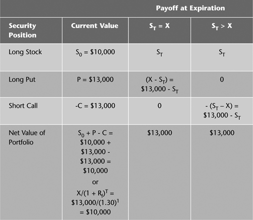
This tells us that a long stock position can be synthetically replicated by forming a portfolio of a long call, a long T-bill with face value X, and a short put. How do we prove that this truly replicates the cash flow profile of a long stock position? This is done by showing that the initial cash flow generated by the synthetic portfolio is the same as that on a long stock and by showing that the cash flows of the synthetic portfolio at the position’s expiration date match those of a long stock.

Table 5.4 shows that the cash flows are indeed replicated properly. If the individual securities are all properly priced, the initial value of the synthetic portfolio is priced such that S₀ = C + X/(1 + R_f)^T – P, or $30.35 = $1.80 + $29.96 – $1.41. This is our goal.

Table 5.4. Creating a Synthetic Long Stock Using Put-Call Parity

Furthermore, at expiration the net value of the synthetic portfolio is S_T, which replicates the value of a long stock position at that point in time. The table shows that the initial value of the synthetic portfolio is the same as that of a long stock, which is $30.35. It also shows that the net cash flows of the synthetic portfolio at the expiration date match those on a long stock, which is S_T in each case. This illustrates the general method of replicating a position synthetically. Obviously, the same approach may be used to form portfolios that replicate individual calls, puts, or T-bills—either long or short.

It is interesting to consider the special impact that the T-bill position has on synthetic portfolios. Because the T-bill has a constant payoff at maturity, its effect on the cash flows is always just a constant. In other words, the T-bill does not affect the responsiveness of the synthetic portfolio’s cash flows to moves in the underlying stock. Thus, it is common to omit the T-bill when an investor is comfortable just creating a mimicking portfolio at lower cost than creating a synthetic replicating portfolio.

Using Put-Call Parity to Understand Basic Option/Stock Strategies

We considered how put-call parity provides a framework for forming synthetic portfolios that can replicate individual or combined security positions. Certain combinations of securities in a portfolio constitute a strategy. Here we extend our prior discussion of creating synthetic positions using put-call parity by considering two common option/stock strategies: covered call and protective put.

Put-Call Parity and the Covered Call Strategy

The covered call strategy consists of long stock and short calls on the same stock in a 1:1 mix. In other words, the classic covered call strategy holds a short call position that contains the same number of shares of stock that the investor owns. Consider two commonly offered motivations for this strategy. First, perhaps an investor is long a stock and fears that its price will drop, but he does not want to sell the shares now. Hence, the short call’s premium provides income that offers some downside protection on the exposed long stock. In other words, the premium income generated by the short call provides a buffer that defers losses on the long stock position. Thus, the primary motive is to protect the long stock position.

Second, perhaps an investor is unhappy with the return on his stock, so he decides to generate additional income by selling call options on that position. Similarly, an investor might expect the stock to go up only modestly, so he decides to write an “out-of-the-money” call to pick up some additional income.⁸ When the argument is presented as a “money for nothing” transaction, it is flawed. This is because the sale of call options on a preexisting long stock position gives up something of value. Indeed, the short calls establish the maximum price at which the investor can sell the underlying shares of stock. In other words, if the price of the stock exceeds the exercise price of the short call, the option is exercised, and the stock is sold at that exercise price. This imposes a potentially significant opportunity cost on an investor by imposing a ceiling on the maximum sale price. Think of the strategy as trading additional downside protection for reduced upside price appreciation potential. However, there is really no complete downside protection with the covered call strategy. Specifically, as soon as the stock price drops below the exercise price by more than the option premium received, the protection is exhausted, and the investor is exposed to all further declines in the stock’s price.

Let’s develop the insight that put-call parity provides into the construction of the covered call strategy. The analysis is limited to European options and considers cash flows only at inception and termination of the position at expiration. Our primary goal is to show how put-call parity yields insight into strategy formulation. Thus, no attempt is made to explore the covered call strategy exhaustively.

Recall that put-call parity was presented earlier as S₀ + P = C + X/(1 + R_f)^T. Let’s continue to use the previously presented YHOO data. Thus, the classic covered call strategy of a matched long stock, short call option position is revealed by restating the put-call parity relation as follows:

S₀ – C = X/(1 + R_f)^T – P or $30.35 – $1.80 = $29.96 – $1.41 = $28.55

Thus, the covered call strategy is equivalent to or may be synthetically replicated as a long T-bill and a short put option. This equivalence helps us better understand the nature and effectiveness of the covered call strategy. Note that the break-even price of the long stock alone is its purchase price of $30.35. The sale of the call reduces the break-even point to $30.35 – $1.80 = $28.55.

Remember that one rationale for the covered call is to provide some downside protection against a decline in the underlying stock. This provides two important observations that afford us some intuition. First, the short call provides income that protects the long position somewhat. Importantly, the risk of the short call is offset by the long stock position, because the investor is not exposed to the risk of buying the underlying stock at increasingly higher prices. This is the risk an investor would be exposed to if he had written a “naked” call. However, the underlying stock is already owned, so the purchase price is already known. The only risk is the price at which the long stock will eventually be sold, the maximum of which is determined by the exercise price on the short calls.

Second, the nature of the synthetic portfolio reinforces our intuition. Recall that the synthetic portfolio is long a T-bill and short a put. The long T-bill produces a certain payoff of X on the expiration date, and the short put option provides additional return through the premium income it generates. However, if the stock’s price drops, the short put option becomes more valuable, but to the detriment of the put writer. Consequently, the covered call strategy and its synthetic portfolio of long T-bill, short put are similar in that both have options that provide income that buffers the loss exposure associated with stock price declines.

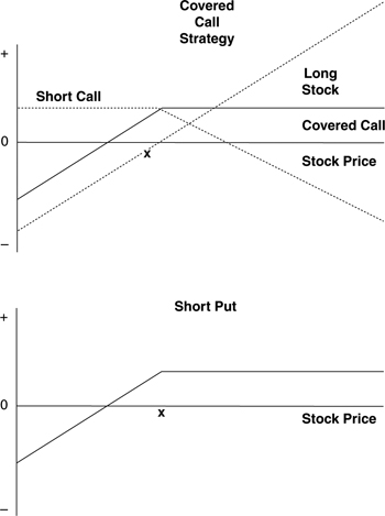
Figure 5.1 shows the intuition yielded by applying the put-call framework to the analysis of the covered call strategy at expiration. Notice that the shape of the covered call strategy is quite similar to that of the short put. As discussed, the T-bill position in put-call parity may be viewed as a constant. In other words, its presence or absence in a portfolio changes only the level of the cash flows, not the responsiveness of the cash flows to changes in the underlying stock price. Thus, the T-bill position changes the level but not the shape of the profit/loss diagram. In terms of the put-call parity relation, a covered call strategy is equivalent to a long T-bill and a short put. Given that the T-bill can be dropped while still preserving the strategy’s general character, we should expect the covered call profit/loss diagram to look like that of a short put. This is confirmed by the indicated figures.

Figure 5.1. Profit/Loss Potential on a Covered Call Versus a Short Put Position

So what is the significance of the observation that put-call parity reveals synthetic positions and comparable strategies? Interestingly, we see one of the most important observations in arbitrage analysis in general and derivatives strategy in particular. The same strategic goal can be accomplished using more than one method.

However, truly equivalent approaches must be priced equivalently. Thus, put-call parity is a lens through which we may see equivalent strategies and determine whether pricing is appropriate.

Put-Call Parity and the Protective Put Strategy

The protective put strategy consists of long stock and long puts on the same stock in a 1:1 mix. Similar to the motivation for the covered call strategy, the protective put may be used by an investor who is long a stock and fears that its price will drop but who does not want to sell the shares now. Hence, the long put is purchased so that the investor does not have to sell below the price chosen as the exercise price. Thus, loss exposure on the long stock position is bounded on the downside. Importantly, the put provides downside protection but does not limit the maximum price at which the underlying stock can be sold. Of course, if the stock’s price appreciates, the investor’s net profit will be reduced by the amount invested in the long put.

While the protective put requires the investor to pay the put premium, the covered call investor receives the premium income provided by the sale of the call option. The protective put strategy is like buying insurance. The put premium is the cost of the insurance. Like any insurance policy, it pays off only if you receive bad news. If nothing bad happens, you have paid the insurance premium but received nothing in return other than the peace of mind of having been insured. Thus, the strategy is like buying homeowner’s insurance and finding that your house did not burn down during the policy’s life. You pay a relatively small, certain amount rather than face the risk of a large potential loss if your house burns down. So good news, bad news—but more good than bad.

Let’s develop the insight that put-call parity provides into the construction of the protective put strategy. Again, we limit the analysis to European options and consider cash flows only at inception and expiration. Furthermore, our primary goal remains showing how put-call parity yields insight into the strategy, so we do not explore all the nuances of the protective put strategy.

Recall that put-call parity was previously presented as:

S₀ + P = C + X/(1 + R_f)^T

Thus, the protective put strategy of a matched long stock, long put option position is present in the original statement of put-call parity relation. No restatement is needed. Thus, the protective put strategy may be synthetically replicated as a long call option and a long T-bill. In terms of the YHOO data, the initial value of the synthetic put is:

$30.35 + $1.41 = $1.80 + $29.96 = $31.76

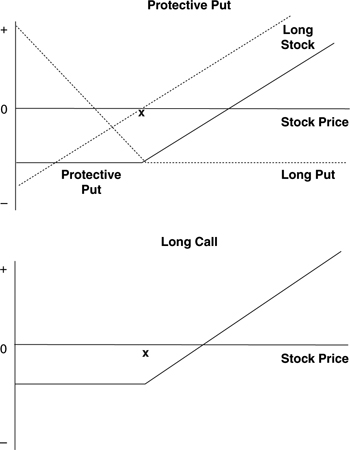
Figure 5.2 shows the relationship between put-call parity and the protective put strategy. As expected, the shape of the protective put strategy is similar to that of the long call. As discussed, the T-bill position in put-call parity may be viewed as a constant. Thus, the T-bill position changes the level but not the shape of the profit/loss diagram. In terms of the put-call parity relation, a protective put strategy is equivalent to a long call and a long T-bill. Given that the T-bill can be dropped without changing the strategy’s basic shape, we expect the protective put profit/loss diagram to look like that of a long call. This is confirmed in Figure 5.2. The breakeven on the long stock is $30.35 when held alone but is increased to $31.76 by the purchase of the put. This is because the price of the stock must rise enough to recoup the cost of the premium paid for the insurance afforded by the protective put strategy before breaking even.

Figure 5.2. Profit/Loss Potential on a Protective Put Versus a Long Call Position

Summary

This chapter presented the put-call parity relation, which relies on arbitrage to portray the relationship between call and put prices, the underlying stock price, the exercise price, the risk-free rate, and the time to expiration for European options. It then showed how to exploit deviations from the predicted relationship using arbitrage strategies and explained how the relationship can be used to create synthetic securities. This chapter also showed how put-call parity lends insight into basic option/stock combination strategies such as the covered call and protective put.

Put-call parity for European options may be stated as follows:

S₀ + P = C + X/(1 + R_f)^T

The relationship should hold because deviations create arbitrage opportunities that can be exploited, thereby returning the prices to no-arbitrage, steady-state values. The chapter provided an example in which the stock/put portfolio was overvalued relative to the call/T-bill portfolio. This was exploited by selling short the stock/put portfolio and hedging that investment by buying the call/T-bill portfolio. The proceeds of the short sale exceeded the cost of hedging the position with the call/T-bill portfolio. Thus, the arbitrage strategy generates an initial cash inflow, which meets the self-financing requirement of arbitrage. The strategy is also riskless. The ability to construct such an arbitrage strategy when put-call parity is violated demonstrates why the relationship is expected to hold.

This chapter showed that put-call parity provides insight into how synthetic and mimicking portfolios can be created. A synthetic portfolio offers the same cash flow pattern and the same appropriate value as the security position it replicates. In contrast, a mimicking portfolio provides the same general, but not exact, cash flow pattern as the security position it mimics, but not necessarily at the same value. The general method of synthetic portfolio formation was illustrated for a long stock position. Rearranging put-call parity indicates that the synthetic portfolio for a long stock position is C + X/(1 + R_f)^T – P. Thus, a long stock position can be synthetically replicated by forming a portfolio of a long call, a long T-bill with face value X, and a short put. Analysis showed that the initial cash flow generated by the synthetic portfolio is the same as that on a long stock and showed that the cash flows of the synthetic portfolio at the expiration date of the position match those on a long stock. Thus, if it barks like a dog and wags its tail like a dog, it’s probably a dog.

The chapter concluded with a discussion of how put-call parity provides insight into basic stock/option combination strategies.

The framework was applied to the examples of the covered call and protective put strategies. Put-call parity reveals synthetic portfolios that afford insight into the nature of each strategy.

Endnotes

¹ As quoted in Lowenstein (2000, p. 116), which cites “Black-Scholes Pair Win Nobel: Derivative Work Paid Off for Professors Who Made Fortune from Investment in Wall Street Hedge Fund,” Daily Telegraph, October 15, 1997.

² An option is a contract between a buyer (holder) and a seller (writer) that gives the holder the right—not the obligation—to buy or sell a given commodity or security at a predetermined price on an agreed-upon future date. The option to buy is referred to as a call, and the option to sell is referred to as a put. The option buyer pays the option seller the option price or premium for the given right. The writer of the option is obligated to do what the option holder decides to do. If the call owner exercises the contract, the call writer is obligated to deliver the underlying asset in return for the contracted price. A contract that can be exercised at any time, up to and including the expiration date, is called an American option, and a contract that can be exercised only on the expiration date is called a European option. To focus on the nature of arbitrage, the analysis is restricted to European options on nondividend-paying stocks. Put-call parity also can be extended to include forwards or futures and options on forwards or futures.

³ The intrinsic value of an option is the difference between the stock price and the exercise price if the difference is positive, and zero otherwise. For example, a call option with an exercise price of $45 on a stock selling for $50 has an intrinsic value of $5. A put with the same characteristics has an intrinsic value of 0. Any excess of the option premium beyond the intrinsic value is called speculative or time value. This reflects the speculation that the option will become more valuable as expiration approaches. Thus, if the call in the example sold for $6, that would imply a speculative value of $1. On the expiration date, an option has no speculative value, because no time is left to accrue more value.

⁴ One of the key observations of option pricing theory is that it is possible to combine stock and call options or stock and put options in a way that provides a certain riskless rate of return. Thus, including the risk-free rate through a T-bill, put-call parity may be thought of as capturing the ability to form a riskless hedge with these positions and also as reflecting the time value of money over the period until a European option can be exercised.

⁵ See Knoll (2002) for an interesting discussion of this issue and a more extensive set of examples of regulatory arbitrage.

⁶ See Miller (1991) for more on the sources of financial innovation.

⁷ See Ross, Westerfield, and Jaffe (1999, p. 554) for an example of how the legend of Russell Sage’s creation of synthetic loans has been integrated into a popular finance textbook.

⁸ A call option is “out-of-the-money” if S₀ < X, “in-the-money” if S₀ > X, and “at-the-money” if S₀ = X. Similarly, a put option is “out-of-the-money” if S₀ > X, “in-the-money” if S₀ < X, and “at-the-money” if S₀ = X.