Chapter 4. International Arbitrage

... [O]thers who favour exerting more control over currency trading are making the dangerous assumption that governments know better than markets what the “correct” exchange rate is. In fact there are good reasons to expect governments to make even bigger mistakes. Moreover, financial markets find it a lot easier than governments to admit their mistakes, and to reverse out of them. That is because one of the un-sung beauties of markets is that, unlike governments, they have no pride.

—The Economist¹

The Law of One Price should hold no matter where an asset is traded in the world. Of course, the price of the same good trading in different places should reflect the transportation costs of moving it around the world. However, such legitimate reasons for price differences should not, on average, be arbitraged profitably. Similarly, differences solely due to prices being denominated in different currencies should “wash out” to preclude arbitrage opportunities. This chapter considers how arbitrage in international markets aligns prices and influences the relationship among currency exchange rates in light of international interest rate and inflation differences. In so doing, we show how foreign exchange rates are molded by arbitrage pressures through so-called international parity relations.

Exchange Rates and Inflation

Absolute Purchasing Power Parity

Consider how exchange rates react to differences in the price of the same good trading around the world. The Law of One Price argues that the same good should sell for the same price no matter where it is after adjusting for the “prices” of different currencies. Prices quoted in different currencies only reflect different scales. It’s like measuring lumber in inches, feet, or meters—you can compare the different measures and figure out how long a board “really” is in familiar terms. Similarly, the price of a comparable cup of coffee at Starbucks should be about the same in Chicago and London after adjusting for the U.S. dollar/British pound exchange rate.

Absolute purchasing power parity (PPP) applies the Law of One Price to exchange rates. Rather than applying it to every good, absolute PPP argues that the average price of a representative basket of goods and/or services should be the same in all countries after adjusting for the effect of different currencies. In other words, in fully competitive economies, the real price of a good or service should be the same everywhere. This implies that the equilibrium exchange rate between any two currencies equates the prices of the representative baskets from each country. For example, if the average price of goods in the U.K. increases relative to that in the U.S., the U.S. dollar must depreciate relative to the British pound if the average real cost of goods in the two countries is to remain the same.

In a world without trade impediments, an arbitrage opportunity is created when absolute PPP is violated. For example, assume that the price of corn is $2.07 per bushel in the U.S. while the exchange rate is $1.8025/£ or £0.5548/$. View the exchange rate as the price of one currency in terms of another. Thus, the exchange rate of £0.5548/$ means that it costs 0.5548 British pounds to buy a single U.S. dollar. Alternatively stated, it costs about $1.80 to buy a British pound. For the price of a bushel of corn in the U.K. to be the same as that in the U.S., it would have to sell for $2.07(0.5548) = £1.15. However, what if the price in the U.K. were £1.45? The real price of corn would then be cheaper in the U.S. than in the U.K., which implies an arbitrage opportunity. Investors would obviously want to buy corn at the lower price in the U.S. and sell it at the higher price in the U.K. Using the framework developed in Chapter 1, “Arbitrage, Hedging, and the Law of One Price” and Chapter 2, “Arbitrage in Action,” the preferred strategy is to sell short corn in the U.K. and use the proceeds to buy corn in the U.S. Thus, the price difference could be risklessly locked in using this self-financing strategy. Pursuing this opportunity should put upward pressure on the price of corn in the U.S. and downward pressure on the price in the U.K. Arbitrage efforts should eventually push the prices together on a currency-adjusted basis. As explained next, the exchange rate should adjust to achieve this result.

Empirical evidence indicates that the absolute version of PPP generally does not hold due to market frictions, such as international taxes, tariffs, and import quotas. Furthermore, consumers in different countries tend to prefer different representative baskets of goods and services that are not, by definition, directly comparable. Notwithstanding this evidence, the absolute version of PPP provides a useful starting point for understanding exchange rate determination.

Relative Purchasing Power Parity

Absolute PPP compares average price levels across countries. It argues that exchange rates should equalize average prices on a currency-adjusted basis. By implication, movements in exchange rates over time are also expected to capture differences in the rate of change of the prices of goods and services across countries. Of course, the rate of change in the average level of prices over time is the inflation rate. Relative PPP argues that exchange rate movements should reflect differences in inflation rates between countries. Thus, for the Law of One Price in general and absolute PPP in particular to hold, countries experiencing higher (lower) inflation should expect their currency to depreciate (appreciate) to keep the real price of their goods and services equal to those abroad. In other words, exchange rate movements should offset differences in inflation rates among countries.

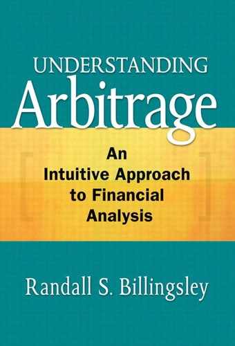
Let’s more precisely examine the specific relationship among the current (spot) exchange rate (S₀), the exchange rate at the end of one period (S_t), the expected inflation rate in the domestic economy (INF_d), and the expected inflation rate in the foreign country (INF_f). Relative PPP states the following:

This assumes that exchange rates are quoted as domestic currency per unit of foreign currency—U.S. dollars per British pounds in this example.² The expression asserts that the ratio of the ending to the beginning of period exchange rates should equal the ratio of the domestic-to-foreign inflation rates in the two countries. Similarly, the difference between the inflation rates in the domestic and foreign economies should be approximately equal to the percentage change in the spot exchange rates:

Reconsider the earlier example of the price of corn in the U.S. and the U.K. What if the U.S. inflation rate over the next year is expected to be 3.7% while the U.K. inflation rate is expected to be only 1.5%? Granting that these respective expected inflation rates apply to the price of corn in each country, the exchange rate in effect a year from now should change to maintain the relative prices of corn in the U.S. and the U.K. If the U.S. dollar does not depreciate to offset the 2.2% difference in expected inflation between the two countries, U.S. corn will be less competitive internationally, and arbitrageurs will move money between the U.K. and the U.S. to exploit the unequal real prices of corn. Relative PPP indicates how much the exchange rate must change to preclude an arbitrage opportunity in light of different inflation rates in two countries. Assuming for present purposes that inflationary expectations are realized, the arbitrage-free new exchange rate is implied by the following:

Thus, the higher rate of inflation in the U.S. should cause the exchange rate to move from its current level of $1.8025/£ to an expected exchange rate of $1.8416/£ in a year. This means that the U.S. dollar will depreciate relative to the British pound because it will take more dollars to buy a pound. Alternatively stated, it will cost fewer pounds to buy a dollar at the end of the year. Thus, the value of the dollar must decline to offset the higher dollar-based corn price in the U.S. relative to the price of corn in the U.K.

The ability of arbitrage to influence exchange rate moves is tempered by uncertainty about future inflation. Pure arbitrage is riskless, which precludes such uncertainty. While arbitrage can still be expected to put pressure on exchange rates in the same manner and direction as just explained, uncertainty concerning future inflation implies that arbitrage transactions will not precisely conform to the rigorous riskless condition that characterizes pure arbitrage.

The common sense of relative PPP is reinforced by applying it to the example of corn prices in the U.S. and the U.K. Remember that the current prices per bushel of corn are $2.07 in the U.S. and £1.15 in the U.K. Given that the expected inflation rate is 3.7% in the U.S. and 1.5% in the U.K., the price of corn is expected to be $2.07 (1.037) = $2.15 in one year in the U.S. and £1.15 (1.015) = £1.17 in one year in the U.K. If the exchange rate does not change over the year, the real price of corn will be higher in the U.S. than in the U.K. In other words, using the current exchange rate of $1.8025/£, the price of corn in the U.S. from the British perspective will be £0.5548/$ ($2.15) = £1.19 in one year rather than the £1.17 that is expected to prevail in light of the U.K. inflation rate over the period.

Although this difference is modest due to the small inflation differential, it is nonetheless illustrative. For the arbitrage to be profitable, an investor must find the price disparity large enough to cover the transactions costs of trading. Such an imbalance would create an opportunity for arbitrageurs to buy corn at a lower price in the U.K. and sell it at a higher real price in the U.S. In contrast, relative PPP asserts that the exchange rate should move from $1.8025/£ to $1.8416/£ to preclude arbitrage. Thus, the expected price of corn in one year, which reflects expected inflation in the U.K. and an accommodating change in the exchange rate, would be 0.5430 ($2.15) = £1.17. Relative PPP consequently predicts that the real price of corn will remain the same in the U.S. and the U.K. even though the countries are expected to experience different inflation rates. This is because the exchange rate movement is expected to preclude arbitrage by offsetting the impact of the inflation differential. Again, the threat of arbitrage imposes structure—this time in international markets in terms of exchange rates and inflation.

Interest Rates and Inflation

Domestic Fisher Interest Rate Relation

PPP relies on arbitrage to discipline the relationship between inflation and exchange rates. Before exploring how exchange rates and interest rates are influenced by arbitrage, it is important to consider the relationship between inflation and interest rates in an international context. This relationship is an extension of the famous domestic Fisher relation that asserts that the nominal interest rate (R_n) results from compounding the real interest rate (R_r) and the expected inflation rate (E(INF)):³

(1 + R_n) = [1 + R_f] [1 + E(INF)]

The nominal interest rate thus reflects the real interest rate, which is absent of the effects of inflation, and the impact of expected inflation. The relation is often presented as a linear approximation in which the nominal interest rate equals the sum of the real interest rate and the expected inflation rate: R_n = R_r + E(INF). For example, a real return of 5% in the presence of 3% expected inflation should be associated with a nominal rate of return of about 8%.

Consider this relationship in light of the inflation rate example data cited earlier. Recall that the expected rates of inflation in the example are 3.7% in the U.S. and 1.5% in the U.K. As is often done, further assume that the real interest rate is the same in both countries, which is 1.3%. What are the implied nominal returns on bonds in the U.S. and the U.K.? Relying on the domestic Fisher relation, the nominal rate of return in the U.S. is [(1.037) (1.013)] – 1 = 5.05%, and the nominal rate of return in the U.K. is [(1.015)(1.013)] – 1 = 2.82%.

International Fisher Interest Rate Relation

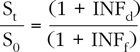
The Fisher relation just discussed portrays the relationship between interest rates and inflation in a domestic economy. Unsurprisingly, the domestic Fisher relation can be extended to understand arbitrage in an international context. As noted, it is common to assume that the real interest rate is constant across countries because the international economy is increasingly integrated. Conversely, unequal real interest rates are expected across countries whose economies are fragmented due to imperfections, such as taxes, tariffs, and import quotas. Given this assumption, the international version of the Fisher relation just divides the relation for the domestic country by the relation for the foreign country:

The left side of the equation is the ratio of 1 plus the nominal interest rates in the domestic (R_d) and the foreign (R_f) country, respectively. On the right side of the equation, neither the numerator nor the denominator includes the real interest rate because it is assumed to be the same in the two countries, which causes it to cancel out.

We can consequently confirm that nominal interest rates in the two countries reflect the inflation rate differential in an arbitrage-free manner using the preceding data. Recalling that the U.S. is defined as the domestic country and the U.K. is defined as the foreign country:

Thus, the ratio of nominal interest rates in the U.S. and the U.K. is equal to the ratio of the inflation rates in the two respective countries.

While the international Fisher relation provides useful insight into long-run international interest rate relationships, it is subject to the same criticisms as absolute PPP along with the complication introduced by possible differences in real interest rates across countries. Nonetheless, it provides a useful example of how arbitrage places boundaries on international rates and prices.

Interest Rates and Exchange Rates

Linking Purchasing Power Parity and the International Fisher Relation

Combining relative PPP and the international Fisher relation reveals the relationship between nominal interest rates and exchange rates. The common link between relative PPP and the international Fisher relation is inflation. On the one hand, relative PPP asserts that changes in exchange rates offset different expected inflation rates in countries to support the Law of One Price. On the other hand, the international Fisher relation posits that nominal interest rates reflect differences in expected inflation rates across countries. Thus, if exchange rates vary with expected inflation and nominal interest rates also vary with inflation, nominal interest rates and exchange rates must be related by virtue of their common link to inflation. This relationship is called interest rate parity, which states that exchange rate movements should offset nominal interest rate differences between countries. In other words, exchange rates should adjust to preclude arbitrage opportunities resulting from interest rate differences.

Uncovered Interest Rate Parity

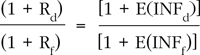
Stating the relationship just discussed in terms of the current spot exchange rate (S₀) and the expected spot exchange rate next year (E(S₁)), interest rate parity is stated as:

When portrayed as the relationship between the current and expected future spot exchange rate, this is called uncovered interest rate parity (UIRP). This is because no effort is made to protect against exchange rate risk when investing in the foreign country; hence, it is uncovered or risky. Our brief discussion of UIRP consequently provides the context for the covered or risk-managed version of interest rate parity.

Consider why UIRP is expected to hold using the data. Recall that S₀ = $1.8025/£, E(S₁) = $1.8416/£, R_d = 5.05%, and R_f = 2.82%. The U.S. is defined as the domestic country, and the U.K. is defined as the foreign country. UIRP asserts that the expected spot exchange rate in one year, E(S₁), should agree with the prediction of relative PPP. Thus:

which is consistent with the results of our prior analysis.

To more clearly see the economic intuition behind UIRP, compare the rates of return from the domestic and foreign perspectives as follows:

This form of UIRP emphasizes that the rate of return from investing abroad depends on the nominal return earned in the foreign market (R_f) and the return associated with investing at one exchange rate (S₀) and repatriating funds at another at the end of the period (E(S₁)). The ratio of E(S₁)-to-S₀ in the preceding expression is 1 plus the expected rate of return from converting the domestic currency into the foreign currency and converting it back into the domestic currency at the end of the year. Similarly, it reflects the rate of return implied by the expected change in the exchange rate over the period.

UIRP yields insight into how arbitrage can moderate the relationship between interest rates and exchange rates. However, it is not true arbitrage because it assumes that an investor seeking to exploit interest rate differentials across countries remains exposed to exchange rate risk over the investment’s time horizon. True arbitrage involves hedging the risk of exchange rate fluctuations over the time horizon an investor is seeking to take advantage of international interest rate differences. Such hedging requires taking a position in a forward or futures contract that locks in the rate at which currencies will be exchanged in the future. We illustrate true arbitrage by examining covered interest rate parity (CIRP), which hedges foreign exchange risk using the forward market.

Covered Interest Rate Parity

CIRP portrays the relationship between the current spot exchange rate, S₀, and a fixed exchange rate for future time t (F_t) specified by a forward contract. Thus, CIRP may be stated as:

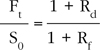
Assuming a one-year period, this is often expressed as:

which indicates that to preclude an arbitrage opportunity, the forward exchange rate should equal the current spot exchange rate multiplied by the ratio of (1 + the domestic nominal rate) to (1 + the foreign nominal interest rates).

Think of the two interest rates as borrowing and lending rates; which is which depends on how CIRP is violated. CIRP says that arbitrageurs will not, on average, profit by merely borrowing money in a country with a lower nominal interest rate and then investing those funds in a country with a higher nominal interest rate. While an investor obviously wants to borrow at the lower rate and lend at the higher rate, CIRP argues that arbitrage will push exchange rates to adjust so that the currency-adjusted rate of return is equal across countries.

CIRP can be restated to emphasize the implied international borrowing and lending decision:

where R_d is the rate of return (borrowing or lending) available in the domestic economy and R_f is the rate of return (borrowing or lending) available in the foreign country. R_d and R_f cannot be meaningfully compared until R_f is adjusted to capture the effect of moving between the domestic and foreign currencies. Thus, the ratio of F₁-to-S₀ may be interpreted as 1 plus the return associated with converting the domestic currency into the foreign currency at S₀. That amount is invested in the foreign currency-denominated security to generate R_f, and then the principal and return generated by the foreign security is converted back into the domestic currency at the future exchange rate F₁. The decision rule is to borrow in the domestic economy and lend in the foreign economy if:

or to borrow in the foreign economy and lend in the domestic economy if:

Thus, R_f can be compared to R_d only after adjusting for the exchange rate effect measured by the relationship between the initial exchange rate S₀ and the forward rate locked in for repatriating the funds F₁. Alternatively stated, the covered interest differential should equal 0 if CIRP holds:

Therefore, at rest, the exchange rate-adjusted interest rates on investments of the same risk should be equal across countries.

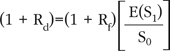
Consider the international borrowing-lending decision indicated by the CIRP framework using the preceding data. Recall that S₀ = $1.8025/£ or £0.5548/$, R_d = 5.05%, R_f = 2.82%, and the U.S. is defined as the domestic country while the U.K. is defined as the foreign country. For simplicity, assume that the forward rate is equal to the expected future spot exchange rate in one period, which is F₁ = $1.8416/£ or £0.5430/$.

Let’s evaluate whether it is best to borrow in the U.K. and invest in the U.S. simply because the rate of return in the U.S. is 5.05% and the rate of return in the U.K. is 2.82%. In other words, we want to determine if the U.S. rate should be viewed as the lending rate and the U.K. rate should be viewed as the borrowing rate simply because the U.S. rate exceeds the U.K. rate. We expect CIRP, as an arbitrage-based argument, to prevent any profit resulting merely from an effort to borrow low and lend high.

The U.S. or domestic return is 5.05%. The exchange rate-adjusted return from borrowing at what appears to be a lower rate in the U.K. is actually the same rate from the U.S. perspective: 1.0282% (1.8416/1.8025) – 1 = 5.05%. Thus, CIRP holds because the exchange rate-adjusted borrowing and lending rates are the same from each country’s perspective. The important lesson is that nominal interest rates cannot be compared meaningfully until they are adjusted to take into account the beginning and ending exchange rates at which money can be invested abroad and repatriated.

To reinforce your understanding of these observations, consider the specific steps involved in attempting to arbitrage the difference between rates in the U.S. and the U.K. For completeness, we examine arbitrage efforts from both the perspectives of U.S. and U.K. investors on a per-unit-of-currency basis. In each case, assume that investors decide to borrow in the U.K. and invest (lend) in the U.S. simply because the nominal rate is lower in the U.K. than in the U.S. First consider the U.S. vantage point. The U.S. investor wants to invest $1 in the U.S. using funds borrowed in the U.K. Thus, $1 worth of pounds is £0.5548 at the indicated spot rate. Given a borrowing rate of R_f = 2.82%, (£0.5548)(1.0282) = £0.5704 will be owed in the U.K. at the end of the year. The $1 invested in the U.S. at R_d = 5.05% will mature to $1.0505 in one year. It costs U.S. investors (£0.5704)($1.8416/£) = $1.0505 to pay off the loan. Thus, U.S.-based investors borrowing in the U.K. and investing in the U.S. earn the U.S. rate of 5.05% after having borrowed in the U.K. at an exchange rate-adjusted rate of 5.05%. Investors consequently have borrowed and invested at the same effective rate. Thus, CIRP holds, and the arbitrage is to no avail.

Now, reconsider the same situation from the perspective of U.K. investors. They want to invest £1 in the U.S. at R_d = 5.05% and borrow in the U.K. at R_f = 2.82%. That £1 will buy (£1)($1.8025/£) = $1.8025 at the current spot rate, which is invested at R_d = 5.05% and matures to ($1.8025)(1.0505) = $1.8935 at the end of the year. This dollar-denominated principal and interest will be converted back into pounds at F₁ = £0.5430/$. Thus, that end-of-year total return converts into ($1.8935)(£0.5430/$) = £1.0282. Thus, the U.K.-based investor starts with £1 and ends up with £1.0282, which is a return of 2.82%. Paying off the U.K.-based loan at 2.82% results in the investor’s having borrowed and invested at the same effective rate. Consequently, despite the effort to obtain a higher return by investing at the higher nominal rate of 5.05% available in the U.S., U.K. investors can earn only the U.K. rate of 2.82%. Once again, CIRP holds, and the arbitrage attempt is ineffective.

Example of Arbitrage Under CIRP

What does it mean if CIRP does not hold? It should imply an arbitrage opportunity. Let’s explore how a profitable arbitrage strategy is designed when a significant violation of CIRP occurs. Again, assume that S₀ = $1.8025, R_f = 2.82%, R_d = 5.05%, and the U.S. is defined as the domestic country while the U.K. is defined as the foreign country. However, now assume that the forward rate is F₁ = $1.9048/£, which is higher than the rate predicted by CIRP.

Compare the borrowing and lending rates implied by these data. Using the previously developed approach:

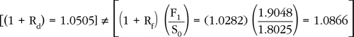
Thus, on an exchange rate-adjusted basis, the rate available in the U.S. is 5.05%, and the rate available in the U.K. is 8.66%. The 8.66% generated by investing in the U.K. consists of a nominal return of 2.82% earned in British pounds and a return of about 5.68% resulting from converting the British pound-denominated principal and interest into U.S. dollars at a more advantageous rate than was in place when the investment was made at the beginning of the year. Thus, the 8.66% is the compound return based on two underlying simple returns: (1.0282)(1.0568). Alternatively stated using an approximation, the covered interest rate differential is not equal to 0; it is 8.66% – 5.05% = 3.61%.

This example again emphasizes that the simple comparison of nominal interest rates need not reveal an imbalance between effective borrowing and lending rates. Indeed, in this case, even though the nominal U.K. rate is only 2.82% while the U.S. rate is 5.05%, we ultimately find it profitable to borrow at the U.S. rate and lend at the U.K. rate. This is because CIRP is violated, which indicates that the exchange rates do not properly offset the interest rate difference.

Table 4.1 portrays the arbitrage strategy from a U.S. investor’s perspective. The strategy is to borrow U.S. dollars at a rate of 5.05%, convert these dollars into British pounds at the spot exchange rate of $1.8025/£ or £0.5548/$, invest these pounds in the British security, and then convert the British pound-denominated principal and interest back into U.S. dollars at the forward exchange rate of $1.9048/£ or £0.5250/$.

Table 4.1. Arbitraging a Violation of Covered Interest Rate Parity

While this example assumes an investment scale of $1,000,000, an arbitrageur would want to invest on as large a scale as possible because the profit is $36,084 per $1,000,000. Interestingly, this profit is about 3.61%, which is equal to the covered interest differential. CIRP is expected to hold as a general rule because its violation creates arbitrage opportunities like this one.

The Relationship Between Covered Interest Rate Parity and the Cost of Carry Model

CIRP relates the spot exchange rate to the forward exchange rate. The cost of carry pricing model presented in Chapter 3, “Cost of Carry Pricing,” relates the spot price to the forward price of a commodity in general, which should include foreign currencies. Consequently, it is reasonable for CIRP to be related to the cost of carry model. Indeed, CIRP is just the cost of carry model restated in terms of currencies.

Recall that the cost of carry model is:

F = S₀ (1 + C)

where F is the forward price, S₀ is the spot price today, and C is the cost of carrying a commodity from today to the delivery date specified in the forward contract. Compare this to the previous statement of CIRP:

The forward and spot rates in the two models are analogous, but they refer to exchange rates in the context of CIRP. We can easily isolate the cost of carry in the above expression as:

Thus, the cost of carry may be viewed as the difference between the forward and spot prices of a commodity as a percentage of the spot price.

Let’s explore the cost of carry implied by CIRP. It may be isolated by restating CIRP using a first-order linear approximation:

The cost of carry stated in percentage terms may be roughly viewed as the difference between the nominal domestic and foreign interest rates. Thus, CIRP argues that the cost of carry should equal the interest rate differential because the difference between the spot and forward exchange rates offsets any potential profit from trying to exploit differences in interest rates between countries.

The relationship between CIRP and the cost of carry model is instructive. However, it is often assumed that the expected future spot exchange rate will, on average, equal the forward rate. Indeed, this assumption was made for simplicity in the prior analysis. However, in Chapter 3, “Cost of Carry Pricing,” we explained that this assumption only holds in the absence of a risk premium. Further, many argue that it is possible to form expectations about the future course of exchange rates based on whether the forward rate is above or below the spot exchange rate. However, addressing CIRP in the context of the cost of carry model suggests that forward and spot exchange rates align themselves in response to interest rate differentials and risk premiums. Thus, placing much faith in forward premiums or discounts as signals of approaching currency appreciation or depreciation is misguided.

Triangular Currency Arbitrage

Cross-Rates, the Law of One Price, and the Nature of Triangular Currency Arbitrage

Our prior discussion views an exchange rate as the price of one currency in terms of another. These prices should adhere to the Law of One Price, which imposes an arbitrage-free structure on the relationship among exchange rates, inflation, and interest rates. Thus, it is reasonable to expect spot currency exchange rates to be consistent with each other as well. For instance, the U.S. dollar can be converted into the British pound, and the British pound can be converted into the Swiss franc. These two exchange rates imply a cross-exchange rate, which provides the exchange rate for converting U.S. dollars into Swiss francs in this example. Thus, U.S. dollars may be converted directly into Swiss francs or may be indirectly converted into Swiss francs by first converting U.S. dollars into British pounds and then converting those British pounds into Swiss francs.

In this context, the Law of One Price asserts that the quoted cross-rate must be the same as the cross-rate implied by the two associated underlying exchange rates. In other words, the exchange rate between the U.S. dollar and the Swiss franc should be the same regardless of whether the conversion is effected directly or indirectly. Because an imbalance between the quoted and implied cross-rates involves three currencies, this is called triangular currency arbitrage. Although exchange rate consistency can be evaluated across more than three currencies, we limit our analysis to the case of three currencies.

Identifying an Arbitrage Opportunity Across Currencies

Let’s first develop a framework for identifying an inconsistency between quoted and implied cross-exchange rates. For example, we can examine the exchange rates between the U.S. dollar and the British pound, between the British pound and the Swiss franc, and between the U.S. dollar and the Swiss franc. The U.S. dollar-to-British pound exchange rate, $/£, and the British pound-to-Swiss franc exchange rate, £/SF, together imply a cross-exchange rate between the U.S. dollar and the Swiss franc, $/SF. More precisely:

To preclude profitable arbitrage, the cross-rate implied by these $/£ and £/SF exchange rates must equal the actual cross-rate quoted in the market.

The easiest way to identify an arbitrage opportunity across the three currencies is to compare the two direct exchange rates and the cross-exchange rate in light of the arbitrage-free condition indicated by simple algebra:

Thus, if the product of the three exchange rates is not equal to 1, an arbitrage opportunity exists.

Consider the example presented in Table 4.2. Evaluating the preceding expression shows that the product of the three exchange rates is 1.0972, which indicates an imbalance. At least one of the exchange rates is too high, because the product should be equal to 1. Consequently, it is worthwhile to design a specific strategy for how you buy and sell the three currencies to exploit the arbitrage opportunity.

Table 4.2. Triangular Currency Arbitrage

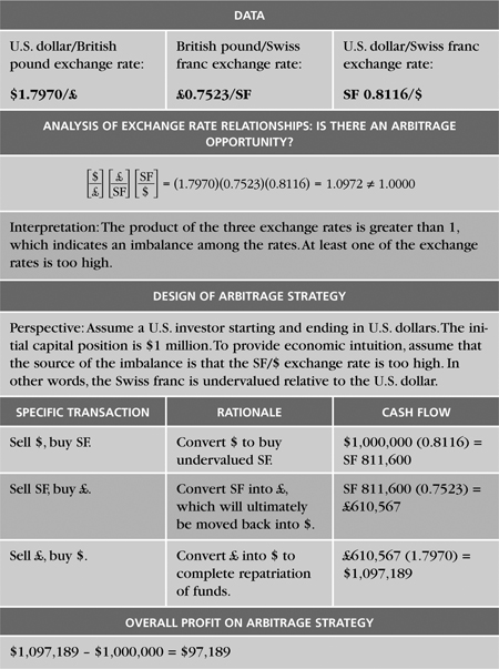
To cultivate an understanding of the underlying currency valuation dynamics, arbitrarily assume that the SF/$ exchange rate is the reason that the product of the three exchange rates is too high. Let’s take the perspective of a U.S. investor who will start and end in U.S. dollars. Simple algebra indicates that this exchange rate is too high for one of two reasons: the Swiss franc quote (numerator) is too high, and/or the U.S. dollar (denominator) is too low. Consider the economic intuition behind these explanations. If the Swiss franc quote is too high for a given U.S. dollar, this implies that the Swiss franc should be lower. This means that it should take fewer Swiss francs to buy a dollar, which indicates that the observed “too high” exchange rate reflects an undervalued Swiss franc relative to the U.S. dollar. Similarly, if the U.S. dollar is too low per Swiss franc, this implies that the U.S. dollar should be higher. Because it should take more U.S. dollars to buy a Swiss franc, the U.S. dollar is overvalued relative to the Swiss franc. Thus, this economic interpretation of the exchange rate product being too high indicates that a U.S. investor should sell overvalued dollars and use them to buy undervalued Swiss francs. The rest of the arbitrage strategy is dictated by the need to move the Swiss francs back into the U.S. dollar. Consequently, the investor should sell Swiss francs and buy British pounds, which would then be converted back into U.S. dollars.

Table 4.2 shows the profit from implementing this strategy. Assuming an initial investment of $1 million, the U.S.-based investor would first convert the U.S. dollars into $1 million (0.8116) = SF 811,600. Wanting to move the funds back into the U.S. dollar, the investor would then sell the Swiss francs and buy SF 811,600 (0.7523) = £610,567. Then he would convert the £610,567 into $1,097,189 at the exchange rate of $1.7970/£. Thus, the U.S.-based investor starts with $1,000,000 and risklessly generates $1,097,189 for a profit of $97,189. This is a return of ($1,097,189/$1,000,000) – 1 = 9.072%. Note that this return is the same as the difference between the product of the three ratios and the balanced, steady-state product of 1, or 1.0972 – 1 = .0972. This confirms the presence of an arbitrage opportunity.

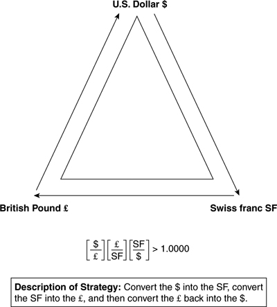
As shown in Figure 4.1, this three-currency arbitrage strategy can be presented graphically as a triangle. Let’s use it to reinforce the lessons of the preceding example. The three corners of the triangle correspond to each of the three currencies. An investor starts and ends in his domestic currency. In this example, that is the U.S. dollar. This consequently dictates the first and last transactions in the arbitrage strategy. The specifics of the strategy—what to buy and sell and in what sequence—are determined by arbitrarily choosing one of the exchange rates and using it to explain the observed deviation of the product of the rates from the steady-state reference of 1. In the example, the product is greater than 1, and the ratio chosen to cultivate our economic intuition is the SF/$ rate. This indicates that the Swiss franc is undervalued and thus that the Swiss franc should be purchased to exploit the imbalance across the rates. The triangle’s value is in visualizing how an investor implements an arbitrage strategy.

Figure 4.1. Example of Triangular Arbitrage

Summary

This chapter has shown how arbitrage influences the relationship among currency exchange rates in light of international interest rate and inflation differences. Foreign exchange rates are structured by arbitrage pressures through international parity relations. Furthermore, this chapter described various arbitrage strategies involving international interest rates and exchange rates.

Absolute purchasing power parity argues that the average price of a representative basket of goods and/or services should be the same in all countries after adjusting for currency effects. Real prices should be the same everywhere because the equilibrium exchange rate between any two currencies equates the prices of the representative consumption baskets from each country. Although trade restrictions such as taxes and import quotas prevent absolute purchasing power from holding perfectly, it is a useful starting point for understanding the relationship between exchange rates and inflation.

Relative purchasing power parity argues that to preclude arbitrage opportunities, exchange rate movements should reflect differences in expected inflation between countries. Thus, countries experiencing higher (lower) inflation should expect their currency to depreciate (appreciate) so as to keep the real price of their goods and services equal. In other words, exchange rate movements should offset differences in inflation rates between countries.

The global relationship between inflation and interest rates can be expressed as an extension of the domestic Fisher relation, which asserts that the nominal interest rate reflects the real interest rate and the expected inflation rate. Combining purchasing power parity and the international Fisher relation reveals the relationship between nominal interest rates and exchange rates. The common link between purchasing power parity and the international Fisher relation is inflation. This link reveals covered interest rate parity, which portrays the relationship between the current spot exchange rate and a fixed future exchange rate specified by a forward or futures contract.

Covered interest rate parity says that arbitrage will not, on average, be profitable if it involves merely borrowing money in a country with a lower nominal interest rate and then investing those funds in a country with a higher nominal interest rate. This is because arbitrage pressures should push exchange rates to the point that the currency-adjusted rate of return is equal across countries. Thus, arbitrage efforts will be worthwhile only if there is a significant difference between domestic and foreign nominal interest rates after currency effects are considered. CIRP is just a special form of the cost of carry model for exchange rates. Comparative analysis of the two models indicates that the cost of carry may be viewed as the interest rate differential.

It is reasonable to expect that spot currency exchange rates for a given base currency will be consistent with each other across all the involved currencies. For example, there should be no price advantage to buying the U.S. dollar directly with British pounds rather than indirectly by first going through another currency to get into British pounds and then into the U.S. dollar. In other words, cross-exchange rates should be consistent with the underlying exchange rates. An inconsistency between the quoted and implied cross-rates involving three currencies may be exploited using a strategy known as triangular currency arbitrage.

Endnotes

¹ “Mahathir, Soros, and the Currency Markets,” September 25, 1997. http://www.economist.com/Story_ID=101043.

² The relation can be extended to consider more or less than one period. Our analysis is limited to one period to emphasize the intuition of the relation and to simplify calculations.

³ See Fisher (1930).

⁴ See Dunbar (2000, pp. 120-123).

⁵ Under Securities and Exchange Commission (SEC) rules in the U.S., hedge funds have less than 100 investors, each of whom are worth at least $1 million. The name “hedge fund” comes from the common practice of both buying and selling short financial assets, thus creating some semblance of a hedge. Unlike mutual funds that tend to charge management fees of 1% or assets under management per year, hedge funds charge that type of fee as well as a fee of 20% or more of profits produced by the fund. The Quantum Fund was legally headquartered in Curacao.