Chapter 2. Arbitrage in Action

Emotion, like instinct not moored in analysis, could be misleading. If you became frightened easily—or were greedy—you couldn’t function effectively as an arbitrageur ... To an outsider, our business might have looked like gambling... It was an investment business built on careful analysis, disciplined judgment—often made under considerable pressure—and the law of averages.

—Robert E. Rubin, former U. S. Secretary of the Treasury, describing risk arbitrage at Goldman Sachs¹

You can best understand arbitrage by considering examples that reflect different perspectives and involve varying degrees of complexity. The first example in this chapter presents the intuitively obvious case of a mispriced individual commodity—gold. The essence of arbitrage is revealed because “sameness” is directly observable and the arbitrage strategy is constructed easily. The second example shows how to exploit mispriced equivalent combinations (or portfolios) of assets. The concept of sameness is extended to evaluate whether various asset combinations produce equivalent outcomes. This example consequently shows how to identify equivalent combinations and illustrates the arbitrage strategy to be used when the underlying individual assets are mispriced relative to a portfolio. The remaining three examples illustrate arbitrage in the context of the capital asset pricing model (CAPM) and the Arbitrage Pricing Theory (APT). This chapter provides general examples of arbitrage in action that are extended in later chapters concerning more specialized arbitrage situations.

Simple Arbitrage of a Mispriced Commodity: Gold in New York City Versus Gold in Hong Kong

What if gold sold at different prices in New York City and Hong Kong? Under what circumstances could the different prices be exploited profitably? Consider what you would do if the price of gold (per troy ounce) was $425 in New York City and $435 in Hong Kong. An arbitrage opportunity exists only if there is no economic reason for the price difference. What would be a legitimate reason for the observed price difference? Assuming that the gold is of comparable quality, one possible reason is the cost of transporting gold between New York City and Hong Kong.

Storage costs, taxes, various government fees, and trading commissions could also explain the price difference. Thus, an economically significant arbitrage opportunity exists only when the price discrepancy is large enough to exploit after taking into account the transactions costs of implementing the arbitrage strategy. There consequently could be a statistically significant difference between the prices (or returns) of the same asset that is economically insignificant in light of transaction costs. Thus, statistical significance does not necessarily imply economic significance.

If the price difference is economically significant after taking into account transaction costs, the arbitrage strategy is to buy gold in New York City, where it is relatively cheap, and sell it in Hong Kong, where it is relatively expensive. Your profit would be $435 – $425, or $10 per ounce less the transaction costs of buying and selling the gold. The combined long and short positions in gold form a hedge that locks in the $10 price difference between Hong Kong and New York City.

How sustainable is the price difference in gold between New York City and Hong Kong? As discussed in Chapter 1, “Arbitrage, Hedging, and the Law of One Price,” we expect the prices of gold in Hong Kong and New York City to converge. In that event, the profit is obtained without a risk of deviating from that $10 difference. Specifically, buying pressure will drive up gold prices in New York City and force gold prices down in Hong Kong. This pressure would bring a sustainable equilibrium price—or a band of prices reflective of transaction costs—for gold on the world market. Thus, prices should converge to the point where any remaining difference reflects only transactions costs that cannot be arbitraged profitably.

Exploiting Mispriced Equivalent Combinations of Assets

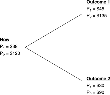
Let’s first examine the arbitrage of mispriced equivalent combinations of assets in the absence of an explicit asset-pricing model. Consider two stocks currently priced at P₁ = $38 and P₂ = $120. Two possible sets of future values are projected for the stocks. In Outcome 1, the first stock is worth P₁= $45, and the second stock is worth P₂ = $135. In Outcome 2, the first stock is worth P₁= $30, and the second stock is worth P₂ = $90. Figure 2.1 portrays these values.

Figure 2.1. Looking for Equivalent Combinations of Stocks

Is there an arbitrage opportunity? This can be determined by examining the relationship between the prices of the two stocks now and their respective values in the two future possible outcomes. This reveals any relationship between the outcomes for the two stocks, which indicates whether they offer equivalent outcomes in some combination.

It is only possible to evaluate whether the stocks are priced correctly relative to one another. No asset valuation model is used to assess whether the absolute prices of either stock are appropriate. The fact that the two stocks have different values in Outcome 1 and Outcome 2 does not definitively reveal an arbitrage opportunity. Conclusive evidence is provided by examining the relationship between the two stocks’ values across outcomes. The comparison of the stocks’ prices across outcomes indicates that P₂ = 3 × P₁ in both Outcome 1 and Outcome 2. However, P₂ currently is greater than 3 × P₁. Consequently, there appears to be an imbalance. Indeed, stock 2 should be viewed as equivalent to three shares of stock 1. The absence of an arbitrage opportunity currently is consistent only with P₂ = 3 × P₁. However, this is not the case, so the prices of stocks 1 and 2 are unbalanced. The Law of One Price is violated because a comparison of the future outcomes reveals that stock 2 is equivalent to three shares of stock 1, and yet the current price of stock 1 is not one-third the price of stock 2. An arbitrage strategy can be designed to profitably exploit the incorrect relative pricing of the two stocks.

What is the appropriate arbitrage strategy? At a current price of only $38, stock 1 is undervalued relative to stock 2’s price of $120. Remember that true arbitrage requires no additional funds and is riskless. Arbitrage strategies sell or sell short overvalued stocks, buy undervalued stocks, and hedge the overall investment position to render it riskless. Because stock 1 is undervalued relative to stock 2, three shares should be bought because this position is equivalent to one share of stock 2. To finance the purchase of three shares of stock 1 and to make the strategy riskless, stock 2 should be sold short. Importantly, this does not necessarily imply that stock 2 is overvalued. The arbitrage strategy exploits the relative undervaluation of stock 1 by buying it and hedges the position by selling short stock 2. Thus, the short sale of stock 2 finances the purchase of stock 1 because the investor is assumed to have access to the proceeds of the short sale. Furthermore, the short sale of stock 2 hedges the overall position against risk because its price in all envisioned future outcomes is always three times that of stock 1.

Consider the cash flows generated by the arbitrage strategy. The three shares of stock 1 cost a total of $38 × 3, or $114, which is more than financed by the short sale of one share of stock 2 for $120. Regardless of which future outcome occurs, the exact amount of money needed to buy back the share of stock 2 that has been sold short will be generated by the sale of your three shares of stock 1. This confirms that the short sale of stock 2 not only finances the purchase of three shares of stock 1 but also hedges the position against risk. Thus, you receive a net cash inflow of $6 ($120 – $114) initially—yet you do not have to come up with any money later!

The arbitrage portfolio is riskless and is comparable to a $6 loan that never has to be repaid. This situation is unsustainable. As in the example concerning mispriced gold, pressure is placed on the prices of stocks 1 and 2 by the act of arbitrage. This should eventually force the price of stock 2, now and in the future, to be consistently three times the price of stock 1 because stock 2 is equivalent to three shares of stock 1. This forces prices to preclude arbitrage.

Arbitrage in the Context of the Capital Asset Pricing Model

Thus far, our arbitrage examples have not relied on any asset pricing model. We have only looked for situations in which the prices of the “same” asset or portfolio differ. Consequently, only relative mispricing has been considered, and no position has been taken concerning whether an asset’s absolute price is correct. However, many investors use an asset valuation model as a benchmark in identifying arbitrage opportunities. We first examine arbitrage in the context of the CAPM.

The CAPM is an equilibrium pricing model. In such models the absence of arbitrage opportunities is part, but not all, of the conditions that describe general equilibrium. The concept of general equilibrium comprehensively describes how asset prices are set.⁵ Thus, the absence of arbitrage opportunities is a necessary but insufficient condition for achieving general equilibrium. The asset pricing model presented in the APT asserts that the lack of arbitrage opportunities is inconsistent with general equilibrium.

However, it does not speak to the broader issue of how asset prices are determined in general. Although the CAPM is an equilibrium model, the APT is not. The APT framework is explored later.

The CAPM relies on a measure of how much a given asset’s returns change in response to changes in the returns on a broad stock market index. This so-called beta (β) measures the risk of a security relative to the overall market. A common benchmark is the S&P 500 Composite Index (S&P 500). Thus, the volatility, β_i, of stock i’s returns, R_i, relative to returns on the indicated proxy for the market, R_m, is measured as:

where Δ = change. The beta of a stock (or a portfolio) consequently measures the percentage change in the asset’s returns associated with a given percentage change in the overall stock market during the measurement period.

The CAPM posits that the appropriate expected rate of return on asset i, E(R_i), depends on the β coefficient as well as on the risk-free rate of return, R_f, and a market-wide risk premium, E(R_i) – R_f. The usual proxy for the risk-free rate in the U.S. is the return on a U.S. Treasury security. Specifically, the relationship is:

E(R_i) = R_f + β_i (R_m – R_f)

For example, consider a stock with a β coefficient of 0.75 when R_f = 4% and E(R_m) = 14%. The CAPM indicates that the appropriate, risk-adjusted rate of return on the stock is 4% + 0.75 (14% – 4%) = 11.5%. Note that the CAPM may be used to price not only individual stocks but also portfolios. The graphic portrayal of the equilibrium trade-off between expected return and risk (β) is known as the Security Market Line (SML).

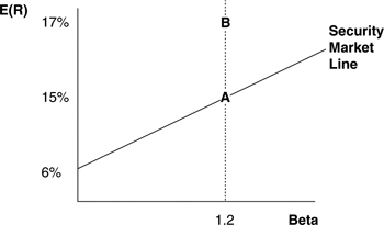
Consider two well-diversified portfolios with the same beta. As shown in Figure 2.2, asset A resides on the SML and has an expected return of 15%, and asset B has an expected return of 17% and is consequently off the SML. Both assets have a β of 1.2. The risk-free return is 6%. The expected return on asset B is too high, which implies that its price is too low. Thus, asset B is undervalued, and asset A is correctly valued. Observe that assets A and B are the same in terms of risk (β = 1.2 for both). Both assets should consequently have the same expected return. Asset A is correctly priced in an absolute sense within the CAPM, asset B is incorrectly priced in an absolute sense, and assets A and B are mispriced relative to one another because they have the same systematic risk but different expected returns. However you look at it, the Law of One Expected Return is violated, and an arbitrage opportunity exists.⁶

Figure 2.2. Capital Asset Pricing Model Perspective on Arbitrage

How should the mispricing of asset B be arbitraged? Buy asset B because it is undervalued, and sell short A to hedge the position. Importantly, asset A is not sold short because it is overvalued. Indeed, asset A is correctly priced. It is sold short to fund the purchase of undervalued asset B and to hedge away the risk of possible adverse price moves in asset B. Assuming that the proceeds from the short sale can be used to fund the purchase of B, the strategy generates an initial net cash inflow because the price of B is less than the price of A. This follows from the fact that the expected return on asset B is higher than that for asset A. The transaction locks in the 2% misvaluation of asset B as a riskless excess return. The excess return is hedged because assets A and B have the same β. In other words, no matter which way the prices of the two assets move, the long/short position locks in the 2% return differential. This means that the position is hedged against the damage done if the entire market fell, thereby bringing down the prices of both assets A and B. Similarly, the position could not benefit from a general upsurge in the market either.

Arbitrage Pricing Theory Perspective

One-Factor Model

As the name suggests, the APT prices assets by focusing on the condition in which arbitrage is precluded for assets and portfolios. Arbitrage is first examined from this perspective using a one-factor model. This is similar but not identical to the CAPM, which asserts that the only relevant source of systematic risk is the broad market itself. However, this does not suggest that the CAPM and the APT make the same assumptions or view equilibrium in the same fashion. After exploring arbitrage from the one-factor perspective, the next example considers arbitrage using a broader multifactor version of the APT. This departs from the prior examples by presenting the arbitrage portfolio as a riskless revision of a previously established portfolio in a way that does not require additional funds. The example illustrates the principle that any portfolio change that involves no incremental risk and requires no investment should provide zero incremental expected returns. Alternatively stated, an arbitrage opportunity exists if incremental expected returns are nonzero in the absence of incremental risk.

Consider the portfolio of three stocks shown in Table 2.1, which presents their expected returns, E(R_i), and sensitivities, b_i, to the one assumed factor or source of risk.⁷ These b coefficients are analogous to the β of the CAPM, except that not every b relates to “the market.” For example, stock 1’s b of 3.2 indicates that a 10% increase (decrease) in the return on the single factor is expected to be associated with a 32% increase (decrease) in stock 1’s return.

Table 2.1. One-Factor APT Arbitrage Data

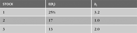
The investment consists of $5 million in stock 1, $5 million in stock 2, and $10 million in stock 3. Thus, the total invested wealth is $20 million. If the expected returns of these three stocks do not properly reflect relative (factor exposure) risk, an arbitrage portfolio can be formed that increases expected return without increasing risk beyond the current level of our portfolio.

An arbitrage opportunity is identified by examining the relationship among the expected returns and risks of the stocks in the portfolio. It is necessary to determine whether any equivalent combinations of securities are not priced equivalently. To describe the portfolio, define W_i as the percentage (weight) of wealth invested in security i. In the current example, W₁ = .25, W₂ = .25, and W₃ = .50. As discussed in Chapter 1, “Arbitrage, Hedging, and the Law of One Price,” long positions have positive weights, and short (or liquidations of existing) positions have negative weights. If the expected return on the current portfolio E(R_p) can be increased by changing the amounts invested in each security without requiring additional funds or increasing risk, an arbitrage opportunity exists. This just restates the previously discussed requirements that true arbitrage is both self-financing and riskless. In this example, the arbitrage portfolio is described by the incremental changes in the amounts invested (weights) in the three assets of the original portfolio. As explained next, the new final portfolio is the addition of the original and arbitrage portfolios.

Let’s more systematically express the constraints that must be satisfied for an arbitrage opportunity. First, the arbitrage portfolio cannot require additional funds. Indicating change with Δ, this requires that ΔW₁ + ΔW₂ + ΔW₃ = 0 in the portfolio. This means that any change in the amounts (weights) invested in the three securities in the portfolio must cancel each other out so that no additional funds are required in modifying the existing portfolio to form the arbitrage position. In other words, additional funds needed to alter the existing long positions (positive weights in the arbitrage portfolio) are offset by the proceeds generated by some sales (negative weights in the arbitrage portfolio) of the existing positions. The arbitrage portfolio has no net sensitivity to the single factor; in other words, it is riskless. A portfolio’s sensitivity is the weighted average of each of the sensitivities of the securities in the portfolio to the one assumed relevant factor. For the portfolio in this example to be riskless, this implies that:

(2.1A.)

or

(2.1B.

Zero nonfactor (unsystematic) risk is assumed.⁸ Thus, the search for an arbitrage opportunity reduces to solving for the amount of money (weight) invested in each of the three assets that simultaneously satisfy the two constraints that no additional funds are required (ΔW₁ + ΔW₂ + ΔW₃ = 0) and that the position be riskless (b₁ΔW₁ + b₂ΔW₂ + b₃ΔW₃ = 0) and yet generate a nonzero incremental expected rate of return. If no such weights can be found that meet these constraints and generate a nonzero expected return, no arbitrage opportunity exists, and prices are presumably in “arbitrage-free” steady state.

The problem contains three unknowns (ΔW₁, ΔW₂, ΔW₃) and two equations (constraints).⁹ Thus, the two constraints may be restated together in terms of the example as follows:

(2.2A.)

(2.2B.)

This system of equations can have an infinite number of solutions. However, if any one solution set of values for ΔW₁, ΔW₂, and ΔW₃ yields a nonzero expected return, an arbitrage opportunity is present. Let’s arbitrarily try a value of ΔW₁ = .15. The complete solution is then found by substituting ΔW₁ = .15 into the no-additional-investment constraining equation (2.2A), solving for ΔW₃ in terms of ΔW₂ and then relying on the no-additional-risk constraining equation (2.2B) to indicate the appropriate value for ΔW_3. The solution process first restates the no-additional-investment constraint:

(2.3A.)

(2.3B.)

This implies that:

ΔW₃ = –.15 – ΔW₂

The no-additional-risk constraint states that:

3.2 (.15) + 1.0ΔW₂ + 2.0 (–.15 – ΔW₂) = 0

This implies that ΔW₂ = .18. Thus, if:

ΔW₁ + ΔW₂ + ΔW₃ = 0

and

ΔW₁ = .15

and

ΔW₂ = .18

then

ΔW₃ = –ΔW₁ – ΔW₂ = –.15 – .18 = –.33

To confirm that both the no-additional-risk and no-additional-investment constraints are satisfied simultaneously, we observe that:

(2.4A.)

and

(2.4B.)

The economic interpretation of this solution is that the long position in stock 1 should be increased by 15%, the long position in stock 2 should be increased by 18%, and the long position in stock 3 should be decreased by one-third to finance the increased amount invested in stocks 1 and 2. In other words, stock 3 is partially liquidated to fund the increased exposure to stocks 1 and 2. All the percentage changes are measured relative to the overall value of the combined portfolio of the three stocks, which is $20 million. Thus, ΔW₁ = .15 implies an increased investment in stock 1 of $20 million × .15 = $3 million, ΔW₂ = .18 implies an increased investment in stock 2 of $20 million × .18 = $3.6 million, and ΔW₃ = –.33 implies a reduction of the investment in stock 3 by $20 million × –.33 = $6.6 million. The no-additional-investment constraint is satisfied because the aggregate increase in the amount invested in stocks 1 and 2 of $6.6 million ($3 million + $3.6 million) is offset by the proceeds generated by the sale of $6.6 million of stock 3.

Is this portfolio an arbitrage candidate? If its incremental expected return is nonzero, an arbitrage opportunity is present. This is determined by calculating the incremental expected return on the portfolio containing the revised investment weights:

(2.5.)

Thus, the revised portfolio weights indicate that the arbitrage portfolio generates a positive incremental expected return of 2.52% while requiring no additional funds and adding no more risk to the original portfolio.

Consider the relationship between the original and arbitrage portfolios presented in Table 2.2. In interpreting the table, focus on the example of stock 1. It is now worth $8 million ($5 million + $3 million). Stock 1 consequently has gone from 25% to 40% of the portfolio. Similarly, stock 2 has increased from 25% to 43% of the portfolio, and stock 3 has decreased from 50% to 17%. This implies the following new expected return and overall factor sensitivity for the portfolio:

(2.6A.)

(2.6B.)

Table 2.2. The Relationship Between the Original and Arbitrage Portfolios

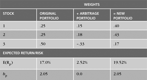
Recall that the expected return on the initial portfolio was 17% and the risk or b was .25(3.2) + .25(1.0) + .50(2.0) = 2.05. Thus, the arbitrage strategy enhances return without increasing the investor’s risk. No significant change in total volatility would be expected if the portfolio were initially well-diversified. In other words, unsystematic risk is trivial.

Two-Factor Model

The preceding examples of asset pricing model-based examples of arbitrage determine expected returns on the basis of a single source of risk—the “market” within the CAPM and an unnamed single factor in the previous APT example. Consider a two-factor APT framework that is representative of more extensively specified models that consider multiple sources of risk.

Assume that assets are priced as portrayed in the general APT approach just presented. The previous model is modified by allowing returns to be generated by two sources of risk. It is reasonable to believe that stock returns are determined by numerous macroeconomic factors such as the rate of inflation, changes in the overall level of interest rates, or changes in the average risk tolerance of investors in the market as the economy moves through the business cycle. Thus, actual portfolio returns, R_p, in this two-factor APT framework should differ from expected returns, E(R_p), due to unexpected changes in two macroeconomic factors, F₁ and F₂, and the sensitivity of the given portfolio to each of the those factors, as measured by b₁ and b₂, and the average firm-specific contribution to unexpected returns, ε_p. More specifically:

(2.7.)

For the sake of the example, consider the first factor to be unanticipated inflation and the second factor to be unanticipated changes in investors’ average risk tolerance. Each of these factors is represented by a factor portfolio, which is a well-diversified portfolio that has a b of 1 on its given source of risk and a b of 0 on the other factor. In other words, the factor portfolio for unanticipated inflation has a b of 1 with respect to the variability in returns induced by unanticipated changes in inflation and a b of 0 with respect to unanticipated changes in investors’ average risk tolerance. The two individual factor portfolios provide benchmarks against which the risk and return of portfolios can be priced in a multifactor context. Assuming that the portfolios in this example are well-diversified, the expected value of the firm-specific component should be 0, or E(ε_p) = 0. We also assume that each of the factor portfolios may be invested in something like an index fund.

Let the expected return on the first-factor portfolio, E(R_F1), be 14% and the expected return on the second-factor portfolio, E(R_F2), be 18%. Assume that the risk-free rate of return R_f is 6%. This implies that the risk premium on Factor 1 is [E(R_F1) – R_f] = 14% – 6% = 8% and that the risk premium on Factor 2 is [E(R_F2) – R_f] = 18% – 6% = 12%. Suppose that portfolio A has a Factor 1 exposure of b_AF1 = 0.85 and a Factor 2 exposure of b_AF2 = 0.35. The two-factor APT model consequently indicates that portfolio A’s expected return should be as follows:

(2.8.)

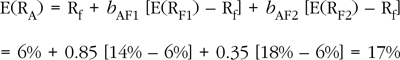
What if portfolio A is mispriced so that its expected return is 19% rather than its appropriate return of 17%? Portfolio A’s expected return is too high, which implies that it is undervalued. This is because the ability to buy at too low a price brings the expectation of too high a rate of return. This violates the Law of One Price and the analogous Law of One Expected Return because a similar portfolio can be built that generates the appropriate expected return of 17%. Similarity in this context is measured by the sensitivities to each of the two factors or sources of risk. Thus, if another portfolio, call it arbitrage portfolio B, with b_F1 = 0.85 and b_F2 = 0.35 can be constructed to yield the appropriate expected return of 17%, the “same thing” will not sell for the same price (expected return), and an arbitrage opportunity will be present. As mentioned earlier, such an opportunity places pressure on asset prices until arbitrage-free prices prevail.

This mispricing may be exploited by taking positions in each of the two-factor portfolios and the risk-free security so as to replicate the riskiness and appropriate expected return of portfolio A. In so doing, we rely on the ability to go long or short and to hedge a position to render it riskless. Furthermore, the arbitrage strategy must not require any net positive initial outlay. As always, the percentages invested in each asset must sum to 100 percent. To determine the riskiness of the arbitrage portfolio, recall that the overall systematic or factor risk of a well-diversified portfolio is equal to the weighted average of the systematic or factor risks of the individual assets constituting the portfolio. The weights are the percentage amount invested in each of the assets relative to the portfolio’s overall market value. Specifically, the goal is to ensure that the same exposure to each of the two factors is achieved wherein b_F1 = 0.85 and b_F2 = 0.35 by investing in the two-factor portfolios and the risk-free security. The essential logic is that we want to go long and short portfolios of equivalent risk but at different prices so that the mispricing can be captured in a riskless, self-financing manner.

Before completing this example of arbitrage using the two-factor APT, let’s consider the concept of calculating portfolio risk in the more straightforward context of the CAPM. Assume that a portfolio consists of $40,000 invested in a stock with a β of 1.25 and $60,000 invested in another stock with a β of 0.95. What is the β_p of the overall portfolio? It is the weighted average of the two βs for the stocks in the portfolio. In this example, it is:

(2.9.)

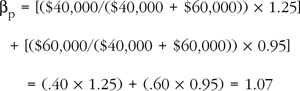
The same approach can be used to determine a portfolio’s overall sensitivity to each of the economic factors in the two-factor APT. Thus, a portfolio’s overall sensitivity to a given factor is the weighted average of the sensitivities to the given factor for each of the securities in the portfolio. As in the CAPM example, the weights are the percentage amounts invested in each of the assets relative to the portfolio’s overall market value.

The preceding two-factor APT example sought to replicate a Factor 1 sensitivity of b_AF1 = 0.85 and a Factor 2 exposure of b_AF2 = 0.35 to replicate the riskiness of portfolio A. Each factor (index) portfolio has, by definition, sensitivity with respect to its own factor of 1. Furthermore, the risk-free security has a sensitivity of zero with respect to all the specified economic factors. This implies that an investor can achieve the desired factor sensitivities by allocating 85% of his money to the Factor 1 portfolio and 35% of his money to the Factor 2 portfolio. The target Factor 1 sensitivity of b_AF1 = 0.85 is obtained because investing 85% in the Factor 1 portfolio, which has a b of 1.00 with respect to Factor 1 by definition, yields a weighted b with respect to Factor 1 of 0.85. Simply put, 0.85 × 1.00 = 0.85 = b_AF1. Similarly, the target Factor 2 sensitivity of b_AF2 = 0.35 is obtained because investing 35% in the Factor 2 portfolio, which also has a b of 1.00 with respect to Factor 2 by definition, yields a weighted b exposure to Factor 2 risk of 0.35 × 1.00 = 0.35 = b_AF2.

You probably are wondering how investing 85% in the Factor 1 portfolio and 35% in the Factor 2 portfolio is possible, because the percentages add up to 120%. Indeed, an investor’s allocations must ultimately sum to 100 percent if we have completely described what a portfolio contains and how it has been financed. Let’s address this apparent contradiction.

We earlier assumed that an investor has access to the funds generated by short sales. Consider that selling short an asset with a positive expected return is like borrowing funds at that expected rate of return. By implication, obtaining funds through the short sale of the risk-free asset is the same as borrowing funds at the risk-free rate. So what is the significance of this observation? The ability to obtain funds through selling short the risk-free asset brings an overall portfolio allocation that appears to be above 100 percent back to the required allocation of only 100 percent of an investor’s money. In other words, the amount allocated to the Factor 1 portfolio is 85%, to the Factor 2 portfolio is 35%, and to the risk-free security is –20%. The investor has invested in two assets (factor portfolios 1 and 2) and sold short the risk-free asset to help finance the overall position.

Now that you understand how to construct arbitrage portfolio B to replicate the risk of undervalued portfolio A, let’s explore how to implement the overall arbitrage strategy and evaluate the expected outcome. Portfolio A is bought because it is undervalued. To render the overall strategy riskless and to eliminate any initial cash outlay, it is necessary to sell short arbitrage portfolio B. The two portfolios have the same risk. Portfolio A has an expected return in excess of portfolio B, which implies that the price of portfolio B exceeds that of portfolio A. Thus, the proceeds generated by the short sale of portfolio B exceed the price of purchasing undervalued portfolio A. Therefore, going long and short portfolios of the same risk is a hedged, riskless position, and yet the strategy generates an initial cash inflow. The strategy consequently meets the requirements for the presence of an arbitrage opportunity; it is riskless and self-financing.

What outcome can you reasonably expect from this strategy? This can be portrayed by comparing the actual returns that will be obtained on each of the two portfolios. Recall from equation 2.7 that R_p = E(R_p) + b₁F₁ + b₂F₂ + ε_p. The actual returns that will be obtained on the portfolios are:

(2.10A.)

(2.10B.)

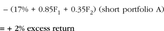
Any variation in the two sources of factor risk cancel each other out because the two portfolios have the same exposure to those factors, and one portfolio is long while the other is short. Thus, as shown in equations 2.10A and 2.10B, the combined positions make up a riskless hedge that captures the 2% difference in the expected returns on portfolios A and B without requiring an initial cash outlay. This is a “money machine,” and the act of arbitrage will push the two portfolios back to the arbitrage-free price level.

Summary

This chapter illustrated the nature of the Law of One Price, the Law of One Expected Return, arbitrage, and hedging using several examples. These concepts were first illustrated using the example of a discrepancy in the price of gold in two locations. We concluded that an arbitrage opportunity is present and exploited it by buying gold where it is cheap and selling short gold where it is expensive. This example showed that arbitrage is riskless, is self-financing, and involves at least one mispriced asset. It is riskless because the position is shown to be perfectly hedged, and it is self-financing because the proceeds from selling the gold short are used to finance the purchase of the gold where it is cheap. Although no asset pricing model was invoked in the example, at least one of the gold prices must be incorrect.

Arbitrage and hedging also were illustrated in the context of asset pricing models. The perspectives of the CAPM and one- and two-factor APT models were presented. These examples showed how asset pricing models can be used to determine the sameness or equivalence of different assets and portfolios. The CAPM and APT examples showed that two portfolios with the same risk are viewed as equivalent for the purpose of identifying arbitrage opportunities. By the Law of One Expected Return, the two portfolios with the same risk must have the same expected return. If equivalent investments do not have equivalent returns, the cheap investment is bought and the expensive is sold in a manner that produces a riskless hedge that is self-financing. Thus, a return in excess of the risk-free rate is produced even though no risk is borne due to the presence of some mispricing.

The examples presented in this chapter implicitly show that the Law of One Price cannot be relied on solely because assets and portfolios with equivalent returns do not necessarily have the same expected future cash flows and therefore need not have the same prices. Thus, the Law of One Price must be restated as the Law of One Expected Return in considering the CAPM and APT. This revised law asserts that equivalent assets should generate the same expected return, which is different from requiring that the same assets have the same prices.

Endnotes

¹ Rubin, Robert E. and Weisberg, Jacob, In an Uncertain World: Tough Choices from Wall Street to Washington (New York: Random House, 2003, pp. 43, 46).

² Based on Lamont and Thaler (2000, p. 230).

³ Lamont and Thaler (2000, p. 266).

⁴ Lamont and Thaler (2000, p. 266).

⁵ While the absence of arbitrage opportunities is consistent with equilibrium, the achievement of general equilibrium satisfies additional conditions. See Fama and Miller (1972) for an extensive discussion of market equilibrium in the theory of finance.

⁶ This example presents expected returns, which implies risk. Thus, there is no guarantee that the ex post returns will equal the estimated ex ante returns. For example, it is possible that some unsystematic (diversifiable) risk that is unrelated to beta will cause the ex ante and ex post returns to differ. However, the fact that the example is for well-diversified portfolios minimizes any concern over the impact of unsystematic risk.

⁷ This example is adapted from the discussion of arbitrage and the APT in Sharpe, Alexander, and Bailey (1999, pp. 283–286).

⁸ This would be easiest to accept if the positions in the portfolio were actually well-diversified portfolios. Nonetheless, we assume that nonfactor risk is not large enough to be a concern and recognize that true arbitrage assumes that this is so as well.

⁹ Alternatively, the problem may be viewed as having a third constraint that the expected incremental return on the arbitrage portfolio must be nonzero. I present the problem with the goal of finding a nonzero expected incremental return rather than viewing it as a constraint.