Chapter 3. Cost of Carry Pricing
The price of an article is charged according to difference in location, time, or risk to which one is exposed in carrying it from one place to another or in causing it to be carried. Neither purchase nor sale according to this principle is unjust.
—St.Thomas Aquinas c. 1264
This chapter extends the arbitrage framework by presenting the cost of carry model approach to identifying and exploiting mispriced positions. The model links two types of prices: spot prices, which are transactions today, and forward and futures prices, which are negotiated today but apply to future transactions. The framework powerfully yet simply reveals when spot and forward or futures prices incorrectly reflect the costs and benefits of the passage of time. After explaining the logic of the cost of carry approach, this chapter presents specific examples of the model for a commodity, silver, and for interest rates.
The Cost of Carry Model: Forward Versus Spot Prices
Pricing Perspective
First consider the cost of carry model from an absolute pricing, currency-denominated perspective. What is a reasonable relationship between the spot (cash) price, S, of a commodity like silver and its forward price, F, for delivery in one year?1 Should the forward price be higher or lower than the spot price? If there is a difference, what is reasonable?
Consider the key source of any difference between spot and futures prices: time. The difference results from the costs and benefits of moving the commodity through time. Costs could include insuring, storing, and financing the silver position over the one-year holding period. Benefits would include any cash flows generated by the asset, such as dividends or interest over the holding period, but these do not apply in the case of silver. Let’s assume that the contracting parties each hold up their end of the bargain, so there is no risk of default. Otherwise, the risk of default would likely be reflected in the pricing of the forward contract. The relative pricing of the spot and forward should express the net cost of carry, which reflects both the costs and benefits of carrying silver over the given year.
Assume that the net carrying cost amounts to C percent, which is dominated by the borrowing cost component for financial assets. Thus, the forward price should equal the spot price grossed up by the cost of “carrying” the spot position of silver at C percent for the indicated time period:
![]()
For example, a spot price of silver of $5.84 per ounce and a net cost of carry of 3% imply a forward price of $5.84 (1.03) = $6.02 for delivery in one year. This forward price covers the cost of carrying the spot position in silver to the delivery date in one year. The forward price is expected to exceed the spot price when there is a positive net cost of carry.2 Thus, the net cost of carry is the cost of financing and holding the commodity over the indicated time period, which is 8¢ per ounce or 3% in this silver example.3
Why should this forward price hold? The current owner of the silver is unwilling to commit to a future sales price less than $6.02 because he could sell the silver today for $5.84, earn 3% on the proceeds over the next year, and have $6.02 at the end of the year. Alternatively, the buyer of the silver through the contract would be unwilling to pay more than $6.02 because he could borrow the current spot price of silver of $5.84, finance the loan at 3% over the next year, and pay off the principal and interest on the loan for $6.02 in a year. Because the buyer is unwilling to pay more than $6.02 and the seller is unwilling to accept less than $6.02, this becomes the steady-state price. This reference point is important because deviations from it imply an arbitrage opportunity.
Rate of Return Perspective: The Implied Repo Rate
Reconsider the cost of carry model from a rate of return perspective. Let’s calculate the return implied by buying silver, holding (carrying) it for one year, and then delivering the silver to cover a short position in the forward market. The result is referred to as the implied repo rate because it is similar to a short-term transaction called a repo, in which a security is sold with the agreement to buy it back later at a higher price. The difference between the purchase and sale prices implies a financing rate for the transaction’s given time horizon. In the context of forward and spot prices, the implied repo rate, R, is:
![]()
If the forward price reflects the mentioned 3% cost of carry, the implied repo rate equals the cost of carry:
![]()
Enforcing the Cost of Carry with Arbitrage
What if the forward price does not properly reflect the cost of carry? Alternatively stated, what if the repo rate is not equal to the cost of carry? This creates an arbitrage opportunity, which is the opportunity to risklessly lock in the difference between the implied repo rate and the cost of carry using a strategy that does not require a positive initial investment. One of two strategies is appropriate: cash and carry or reverse cash and carry.
There are two mispricing possibilities: the forward price is either too high or too low relative to the spot price. It is important to emphasize that this is a relative valuation approach. In other words, the forward price is misvalued relative to the spot price. Thus, any misvaluation originates in the forward, not the spot market. Importantly, no absolute spot pricing model is used to identify mispricing. An example of an absolute pricing model is calculating the present value of the expected future cash flows on a spot position.
Example of Cash and Carry Arbitrage
Consider the case in which the forward price of silver is $6.15. We noted that the appropriate forward price is $6.02 in light of a cost of carry of 3% and a spot price of $5.84. Thus, the forward contract is too high relative to the spot price of silver. Consequently, the forward contract is overvalued relative to the spot price. Two approaches may be used to show that this situation is unsustainable. We first show that this creates an arbitrage opportunity from a pricing perspective. Second, we show that the implied repo rate differs from the financing rate in this case.
Common sense suggests that we sell the forward contract because it is overvalued. However, selling it alone is risky because the price that must be paid to buy the silver in a year is unknown. This is called price risk. As explained in Chapter 1, “Arbitrage, Hedging, and the Law of One Price,” the risk of selling the forward contract can be neutralized by establishing a hedge. In this example, the hedging transaction is to buy the silver today in the spot market and carry it forward for delivery in a year. This eliminates price risk because we then know the total cost of buying the silver to be delivered in a year: the spot price plus the cost of financing that purchase price over the year-long period. And we know the sales price of the silver because it was established by the short forward contract. Thus, because we are long and short the same quantity of silver, any move in the price of silver is self-canceling. Thus, we risklessly lock in the spread between the spot and the forward prices by borrowing to buy spot silver and also selling it forward.
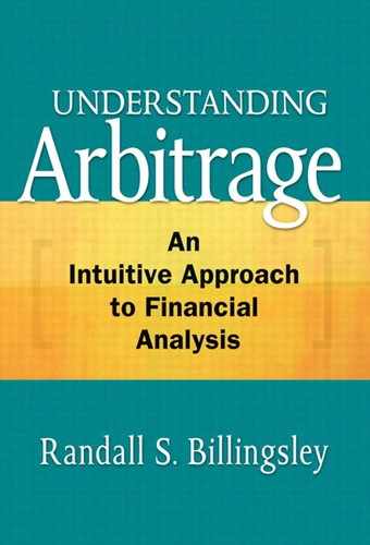
This strategy is called cash and carry arbitrage: buy the commodity in the spot market with borrowed funds, carry (hold) it for one year, and pay off the loan using the proceeds generated by the sale of the commodity under the terms of the forward contract. Table 3.1 summarizes the steps of the strategy using the data for silver on a per-ounce basis.
Table 3.1. Cash and Carry Arbitrage Example for Silver
The strategy meets the required conditions for arbitrage presented in Chapter 1. The purchase of silver in the spot market using borrowed funds neither generates nor requires cash. There is no price risk, and yet the difference between the effective purchase and sale prices implies a return that differs from the risk-free rate. As explained previously, a riskless position that does not generate the risk-free rate of return implies an arbitrage opportunity.
Let’s confirm that the implied repo rate differs from the financing rate in this example:
![]()
This is greater than the 3% cost of carry. The source of the excess return is the forward price being greater than that predicted by the cost of carry model. Thus, as discussed, the appropriate strategy is to sell the overvalued forward contract and hedge the position by buying silver in the spot market with borrowed funds. Because the implied repo rate exceeds the cost of carry, we can carry the silver to the delivery date and still make a profit in excess of the risk-free rate. Thus, we effectively can borrow at the risk-free rate and invest at a rate above the risk-free rate. As noted, the position is riskless and self-financing.
Example of Reverse Cash and Carry Arbitrage
Reconsider the preceding example by assuming that the forward price for silver is only $5.95, which is lower than the $6.02 predicted by the cost of carry model. The forward contract is consequently undervalued relative to the spot price. Once again, we can show that this creates an arbitrage opportunity from both the pricing and implied repo rate perspectives.
We obviously want to buy the forward contract because it is undervalued. However, buying the contract alone is risky because we do not know what the spot price will be when we sell the silver in a year after we buy it through the long forward position. This risk can be neutralized by selling short the silver today in the spot market. As before, we assume that the proceeds of the short sale can be invested at the 3% cost of carry for the one-year time period spanned by the contract. This transaction eliminates price risk because the price at which we sell the silver in the spot market is locked in by the short sale. As in the case of cash and carry arbitrage, any move in the price of silver is self-canceling. This is because we are long (via the long forward position) and short (via the sale of silver in the spot market) the same quantity of silver. Consequently, there is no exposure to the risk that silver prices will increase and thereby bring a loss on our short position, because the price at which we will cover the short is fixed at the long forward position’s price. Thus, we have risklessly locked in the spread between the spot and forward prices. The hedge generates a profit in excess of the risk-free rate because the forward price is less than that indicated by the cost of carry pricing relation.
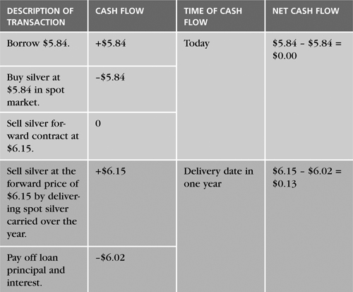
This strategy is called reverse cash and carry arbitrage—buy the forward contract, sell short silver in the spot market and invest the proceeds at the riskless interest rate for one year, and cover the short position in one year using the silver bought at the price specified in the forward contract. Table 3.2 summarizes the steps of this strategy using the data for silver on a per-ounce basis.
Table 3.2. Reverse Cash and Carry Arbitrage Example for Silver
The reverse cash and carry strategy meets the required conditions for arbitrage. The simultaneous short sale of the silver in the spot market and the investment of those proceeds neither generate nor require cash initially. There is no risk because the short sale is covered using the silver purchased at the predetermined forward price at the end of the year. However, the riskless position does not generate the risk-free rate of return, which implies an arbitrage opportunity.
As expected, the implied repo rate differs from the cost of carry in this example:
![]()
which is less than the 3% riskless interest rate. The source of the excess return is the forward price being lower than that predicted by the cost of carry model. Thus, as discussed, the appropriate strategy is to buy the undervalued forward contract and hedge the position by shorting silver in the spot market and investing the proceeds for one year at the cost of carry. Because the implied repo rate is below the riskless interest rate, we effectively can borrow at a rate below the risk-free lending rate. The cash and carry and reverse cash and carry arbitrage strategies are summarized in Table 3.3.
Table 3.3. Summary of Cost of Carry-Based Arbitrage Strategies

Cost of Carry and Interest Rate Arbitrage
The arbitrage strategies just discussed exploit unjustified differences between forward and spot prices, which also imply that the implied repo rate and cost of carry differ. The same approach can be used to explore differences in fixed income security returns across maturities, which is known as the term structure of interest rates. It is common to graphically plot the relationship between spot market yields and maturities for U.S. Treasury securities, resulting in what is called the yield curve. Term structures of interest rate analysis can identify differences in yields across different maturities that reflect violations of the cost of carry relation. This can consequently identify potentially profitable arbitrage opportunities. Such analysis also enhances our understanding of the nature and applicability of the cost of carry pricing framework.
Example of Identifying an Interest Rate Arbitrage Opportunity
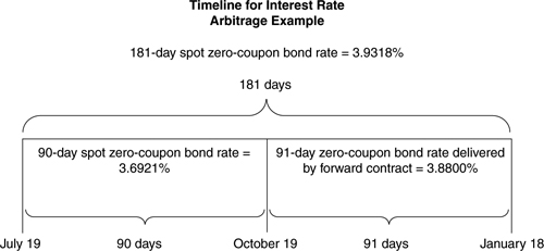
Consider the following data on spot and forward yields observed on July 19:
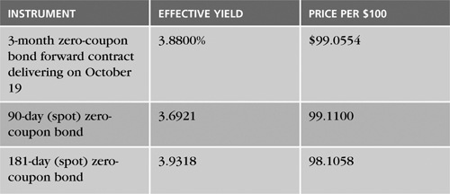
We consider spot and forward positions in zero-coupon bonds with face values of $1 million, which are discount instruments that do not pay coupons. For simplicity, we assume that these securities have no default risk. While this example is most applicable to government securities, such as U.S. Treasury bills (T-bills) and their forward or futures contracts, the analysis may be extended easily to other zero-coupon and coupon-bearing securities.6 Figure 3.1 shows a timeline of the data for this example.
Figure 3.1. Timeline for Interest Rate Arbitrage Example
Designing an Arbitrage Strategy
Consider the insight into financial engineering revealed by analyzing the relationship between spot and futures or forward contract interest rates across the term structure. The goal is to determine whether the relative prices and implied yields of the spot and forward instruments described here are consistent with the Law of One Price and its corollary, the Law of One Expected Return.7 This implies that returns on all positions of comparable risk for the same time period should be the same.
We explain interest rate arbitrage analysis by looking at the preceding example from two different vantage points in time. The first perspective compares the return on the shorter-term spot security (maturity t) with the return on a combined spot/forward position for the same period of time. In the example, we specifically explore whether the forward contract can be combined with a spot position to generate a return over the 90-day period from July 19 to October 19 that differs significantly from the 90-day spot rate of 3.6921%. Because the two investments cover the same time period and have the same risk, they should have the same return. If these returns are different, the cost of carry relationship is violated, and an arbitrage opportunity exists.
Taking the second perspective, the return on the longer-term spot security (maturity T) is compared to the return from investing first in the shorter-term (maturity t) spot security followed by investing in the spot security (maturity T – t) delivered by the forward contract, which matures at time T. An investment maturing at time t followed by an investment for period (T – t) spans the entire longer time period of maturity T: t + (T – t) = T. Because these two investments have the same risk as the spot security maturing at time T, they should jointly generate the same return. Specifically, we compare the return on the longer-term 181-day spot position with the return from investing in the 90-day spot position followed by investing in the 91-day spot zero-coupon bond delivered by the forward contract. Thus, we compare the returns on two different 181-day investments that have the same risk and consequently should have the same returns. If the returns differ, an arbitrage opportunity exists.
Let’s more carefully describe the specific steps in doing interest rate arbitrage analysis from each of the two perspectives. From the first perspective, we start by examining the spot return on a security with a shorter-maturity at time t. Suppose that a forward contract is trading on the same shorter-term security that is to be delivered at time t. Then, we examine the return on a longer-term, otherwise identical spot security, maturing at time T. Thus, T > t. At the delivery date t, the longer-term security will have a remaining maturity of T – t, which is the maturity of the security that will be delivered by the forward contract. Consequently, this security can be used to satisfy the delivery requirement on the forward contract. Given this information, we can check whether the prices and implied returns are arbitrage-free. Specifically, we compare the return on the t-maturity spot security with the return on a combined long position in the T-maturity spot security and a short forward position that delivers at time t. Thus, both positions have a maturity of t. If the returns differ, an arbitrage opportunity exists.
Let’s apply this analytical approach from the first perspective to the data. As of July 19, we examine the spot return on a 90-day security maturing on October 19 (time t), the spot return on a 181-day security maturing on January 18 (time T), and the implied return on a combined spot/forward position spanning the 90-day period from July 19 to October 19. Note that on October 19, the remaining maturity on the 181-day security is 91 days (T – t = 181 – 90 = 91), which is the maturity of the security to be delivered by the forward contract on that date.
Now consider the specific combination of a spot security and the forward contract that yields a return over the 90-day period from July 19 to October 19. If we hold the 181-day security for only 90 days and use it to meet the delivery requirement on a short forward position, we effectively create a synthetic shorter-term security. In other words, we can implement a strategy that shortens the effective maturity of the 181-day security to only 90 days. Similarly, we could structure a strategy to effectively create a longer-term security by buying the 90-day cash instrument and also buying the forward contract. Generalizing this, our analysis demonstrates how to create synthetic maturity (t-period) securities. You will see that the best strategy is determined by the relationship between the return generated by a combined spot/forward contract position and the return on a 90-day spot position, both over the 90-day period from July 19 to October 19.
The first perspective essentially argues that the return on the 90-day spot zero-coupon bond over the period from July 19 to October 19 should equal the implied repo rate on a long spot/short forward position over the same time period. The appropriate spot position to use in calculating the implied repo rate is the longer-term 181-day spot zero-coupon bond, which will have the 91-day maturity on October 19 needed to meet the delivery requirement of the forward contract. Thus, the annualized implied repo rate for the 90-day period is
![]()
which is not equal to the 3.6921% rate on the 90-day spot security. Because the two rates differ, an arbitrage opportunity exists. Given that we view relative mispricing to originate in the forward market, the forward contract price is too high. Thus, an overvalued forward should be exploited using the cash and carry arbitrage strategy, which we will illustrate in detail.
Now, let’s apply the interest rate arbitrage analysis approach from the second perspective to the data. The 181-day return, i181, on the sequence of investing first in the 90-day spot zero-coupon bond yielding i90, and then in the 91-day spot zero-coupon bond yielding f91, delivered by the forward contract on October 19, will provide a 181-day return, i181, of:
![]()
This periodic rate may be restated on an annualized basis as (1.01860)365/181 – 1 = 3.7863%. This is less than the 181-day spot rate of 3.9318%. Thus, an arbitrage opportunity exists because the two rates are different. Given that we once again attribute misvaluation to only the forward market, the fact that the 90-day spot/91-day forward sequential investment strategy produces a return that is lower than the competing 181-day spot position indicates that the return on the forward contract is too low. In other words, if the forward return is too low, its price must be too high.
To reinforce the usefulness of this second perspective, let’s reexamine equation 3.7. We observed that to be arbitrage-free, an investor should be able to earn the same return on the sequence of investing first in the 90-day spot zero-coupon bond and then in the 91-day spot zero-coupon bond delivered by the forward contract as the return on the 181-day spot position. We can further explore this point by restating equation 3.7 to solve for the no-arbitrage 91-day forward contract rate implied by the 181- and 90-day spot rates:
![]()
The annualized implied arbitrage-free forward rate is (1.010236)365/91 – 1 = 4.1694%. However, the quoted 91-day zero-coupon forward rate is only 3.88%. The forward rate implied by the spot term structure should be the same as the quoted forward rate that applies to the same 91-day period in the absence of an arbitrage opportunity. Given that the effective yields are unequal, an arbitrage opportunity exists. The fact that the quoted forward rate is lower than the arbitrage-free forward rate implied by the spot term structure indicates that the quoted price of the forward contract is too high. Indeed, this corroborates our prior finding that the forward contract is overvalued and that the cash and carry arbitrage strategy is appropriate.
It is important to note that the analytical perspectives discussed here are complementary. Each answers the same question, which is whether an arbitrage opportunity exists. Let’s now explore the cash and carry and reverse cash and carry interest rate arbitrage strategies in more detail.
Example of Cash and Carry Interest Rate Arbitrage
Let’s create a synthetic 90-day position for the period from July 19 to October 19 using the preceding data. We will use this strategy to exploit the overvalued forward contract. The 90-day spot position is replicated by selling short the zero-coupon bond forward contract and using borrowed funds to buy a spot zero-coupon bond that can be delivered to meet the requirement of the short forward position. As discussed, it is appropriate to buy the 181-day spot zero-coupon bond because in 90 days its remaining maturity will be 91 days, which satisfies the delivery requirement of the short forward contract. This combined position meets the required conditions for an arbitrage strategy because it is riskless and self-financing. The position is riskless because the purchase price of the spot security and the sales price of the short forward position are each established and known. It is self-financing because the purchase price of the spot security is borrowed. This spot/forward combination is the previously discussed cash and carry arbitrage strategy as applied to fixed-income instruments.
Let’s more explicitly describe the steps of implementing the cash and carry strategy. First, on July 19, we borrow the current purchase price of $981,058 for the 181-day spot zero-coupon bond with $1 million face value at its maturity at the 90-day rate of 3.6921%.8 As discussed, we buy this security to meet the delivery requirement resulting from our sale of the forward contract, which requires us to deliver a 91-day zero-coupon bond in 90 days. Consistent with the earlier discussion, we carry the spot zero-coupon bond to hedge the risk of the arbitrage transaction. Second, we sell short the zero-coupon forward contract that pays $990,554 for the delivery of a 91-day spot zero-coupon bond on October 19. No cash changes hands at the inception of the forward contract on July 19.
On the delivery date of October 19, we deliver the original 181-day spot security, which then has a remaining maturity of 91 days. We repay our 90-day loan, which costs us $981,058 (1.036921)90/365 ≈ $989,868. As noted, we receive $990,554 for delivering the spot security. Thus, the arbitrage profit is $990,554 – $989,868 = $686.9
Example of Reverse Cash and Carry Interest Rate Arbitrage
Reconsider the preceding example by assuming that the effective yield on the forward contract is 4.45%, which implies a quoted price per $100 of $98.9204, for a total contract price of $989,204. The implied repo rate over the 90-day period from July 19 to October 19 is now:
![]()
which is lower than the 3.6921% on the 90-day spot security. Relying on the same logic as before, the first perspective consequently indicates that the forward contract is undervalued. The second perspective indicates that the 181-day return, i181, on the sequence of investing first in the 90-day spot zero-coupon bond yielding i90, and then in the 91-day spot zero-coupon bond yielding f91 delivered by the forward contract on October 19, will provide a 181-day return, i181, of:
![]()
This periodic rate implies an annualized rate of (1.01999)365/181 – 1 = 4.0721%. This is greater than the 181-day spot rate of 3.9318%. As expected, the fact that the 181-day spot/forward sequential investment strategy produces a return that is higher than the competing 181-day spot position indicates that the return on the forward contract is too high and that its price is too low.
We also observe that the modified example provides a quoted forward contract yield of 4.45%, which is higher than the 4.1694% no-arbitrage forward rate implied by the current term structure. While arbitrage consequently once again appears feasible, the fact that the implied no-arbitrage forward rate is lower than the quoted forward contract yield implies that the forward contract is undervalued. The appropriate strategy consequently is the reverse cash and carry arbitrage. Let’s examine this strategy in more detail to reinforce your understanding of cost of carry-based interest rate arbitrage.
The strategy is implemented by buying the undervalued zero-coupon bond forward contract today at $989,204. Yet holding this position alone exposes us to the risk of a decline in the spot price of zero-coupon bonds by the delivery date. So we sell short the 181-day spot zero-coupon bond today at a yield of 3.9318% to lock in the sales price, which is currently $981,058. This amounts to borrowing money. We then invest the proceeds of the short sale by buying the 3.6921%, 90-day spot zero-coupon bond that matures on October 19. Admittedly, this is a bit artificial, because we assume that part of a zero-coupon bond can be bought. In other words, the “whole” zero-coupon bond sells for $991,100, but we want only $981,058 of it so as to match the current price of the 181-day zero-coupon bond. On the delivery day, October 19, we collect the return on the invested proceeds of the previously-shorted 181-day zero-coupon bond, which is $981,058 (1.036921)90/365 ≈ $989,868. We also pay the contract price of $989,204 to take delivery of the 91-day zero-coupon bond under the forward contract commitment. Our arbitrage profit is $989,868 – $989,204 = $664. There are no other net cash flows on the position because on January 18 we collect the $1 million from the maturing zero-coupon bond and use the proceeds to pay the $1 million due on the maturing loan.
Practical Limitations
Arbitrage strategies should be evaluated in light of four practical market imperfections. First, arbitrage is limited by the fact that the repo rate typically is not fixed for the strategy’s full-time period and that it is expected to exceed the risk-free rate. Second, it is possible that an investor will not have access to the full proceeds of a short sale. This would limit the ability to implement a reverse cash and carry arbitrage strategy. Third, the analysis does not capture the potentially significant effect of transaction costs on the profitability of the arbitrage strategies. Fourth, some goods cannot be stored and consequently cannot be carried over time for future delivery. However, this should not be an issue in the example concerning zero-coupon bonds. The basic effect of these frictions is to create a band around the arbitrage-free price or interest rate.
Summary
This chapter presented the cost of carry approach to identifying and exploiting mispriced positions. This useful, simple framework portrays the appropriate relationship between spot and forward or future prices. Properly priced forward/futures contracts reflect the costs and benefits of carrying a spot market commodity or security over time. The cost of carry model was illustrated in this chapter using the examples of a commodity, silver, and interest rates.
The cost of carry model was viewed from the perspectives of both pricing and rate of return. The pricing approach explicitly relates forward price to the spot price as intermediated by the cost of carrying the commodity over time. The difference between the purchase and sale prices also implies a financing rate for the transaction’s given time horizon, which is known as the implied repo rate. If the forward price does not properly reflect the cost of carry, an arbitrage opportunity exists. Thus, it is possible to risklessly lock in the difference between the implied repo rate and the cost of carry using a strategy that does not require a positive initial investment. One of two strategies is appropriate: cash and carry arbitrage or reverse cash and carry arbitrage.
There are two mispricing possibilities: the forward price is either overvalued or undervalued. If the contract is overvalued, a cash and carry arbitrage is appropriate. This is implemented by buying the commodity in the spot market with borrowed funds, carrying (holding) it until the delivery date, and paying off the loan using the proceeds generated by the sale of the commodity under the terms of the contract. If the forward price is undervalued, the reverse cash and carry arbitrage strategy is appropriate. This is implemented by buying the forward contract, selling short silver in the spot market and investing the proceeds at the cost of carry over the time until delivery, and covering the short position using the commodity bought at the price specified in the forward contract.
Arbitrage analysis also helps you better understand the term structure of interest rates. Term structure of interest rate analysis can identify unjustified differences in yields across different maturities that reflect violations of the cost of carry relation. Such analysis may identify potentially profitable arbitrage opportunities. This chapter illustrated the application of both the cash and carry and the reverse cash and carry arbitrage strategies in the context of term structure of interest rate analysis. Interestingly, these strategies can be used to create synthetic maturity securities.
This chapter concluded with an overview of practical market imperfections that influence the implementation of cost of carry-based arbitrage strategies. These imperfections include transactions costs and limited access to the proceeds generated by short sales. The general effect of these frictions is to create a band around the arbitrage-free price or interest rate.
Endnotes
1 A forward contract is a customized commitment to either make (short) or take (long) delivery of a commodity or security of a given quality at a given price at a future point in time. As customized contracts, forwards are traded over the counter. A futures contract is a comparable but standardized exchange-traded contract. In contrast to forward contracts, futures contracts are marked-to-market daily to allocate the profits implied by the day’s price change between the long and short sides. Because forward contracts are not marked-to-market over their life, there are no cash flows until the delivery date. Rather than referring to both forward and futures prices throughout the subsequent discussion, I refer primarily to forward contracts and indicate when a relationship applies differently to futures.
2 It is possible for the forward price to be less than the spot price when an actual or expected shortage forces the spot price up. Consequently, a non-pecuniary “convenience yield” is associated with holding the spot commodity that exceeds the net cost of carry.
3 For simplicity, I do not consider commodities or securities that provide cash inflows over the life of a contract. The effect of such cash inflows would be to decrease the net cost of carry and the forward price.
4 See McDonald (2003, p. 119–198) for an interesting comparison of stock and commodity forwards and futures.
5 If the stock paid dividends, the net cost of carry would decrease, thereby decreasing both the forward and the expected future spot prices. Thus, the results of our analysis would remain the same.
6 Related instruments, such as T-bill and Eurodollar, futures trade on the Chicago Mercantile Exchange (CME). See the CME’s web site for information on these instruments and discount pricing conventions (http://cme.com). See Kolb (1999, pp. 126–130) for comparable T-bill arbitrage examples.
7 I purposely do not rely on the Pure Expectations Theory (PET) of the term structure in designing or implementing interest rate arbitrage strategies. For more on why this is appropriate, see Chance and Rich (2001).
8 Of course, this borrowing rate might not be available to all investors.
9 Yet you may think this amount is insufficient compensation for working through the problem.