Chapter 7. Arbitrage and the (Ir)Relevance of Capital Structure

Looking back now, perhaps we should have put more emphasis on the other, upbeat side of the “nothing matters” coin: showing what doesn’t matter can also show, by implication, what does.

—Merton H. Miller¹

One of the earliest examples of arbitrage-based financial reasoning is the Nobel Prize-winning Modigliani-Miller (M&M) capital structure theory.² This chapter considers the role of arbitrage in assessing the relevance of capital structure decisions in the context of the M&M model. In so doing, the chapter shows how the firm and the securities it issues to finance its operations may be viewed as put and call options. Furthermore, it applies the put-call parity framework developed in Chapter 5, “Put-Call Parity and Arbitrage,” to emphasize the importance of arbitrage in the valuation of alternative capital structures. Thus, this chapter presents the classic theory in light of the previously developed arbitrage framework.

The Essence of the Theory of Capital Structure Valuation

Overview of the Nobel Prize-Winning Framework

Why study an unrealistic, frictionless world in which capital structure does not matter, when realistic frictions seem to imply that it does? As the preceding quote from Professor Miller emphasizes, it is important to understand the conditions under which capital structure does not matter so that it is possible to identify the circumstances under which it does. Furthermore, it is important to understand how arbitrage guides M&M’s classic argument.

M&M’s often-cited Proposition I argues that a firm cannot change the total value of its securities just by splitting cash flow claims into different streams. A firm’s value is determined by its real assets, not by the financial assets (securities) it issues against the cash flows generated by those real assets. Thus, Proposition I separates the firm’s investment and financing decisions and thereby shows that capital structure is irrelevant as long as the firm’s investment decisions are fixed. Indeed, if a firm uses a mix of debt and equity financing, its overall cost of capital will be exactly the same as its cost of equity with all-equity financing. But what ensures that the cost of capital is invariant to capital structure decisions and consequently leaves shareholders indifferent to such financing decisions? As suspected, arbitrage is the answer.

High Finance: Of Pizza, Poultry, and Capital Structure

Before illustrating the underlying arbitrage argument, let’s put a more day-to-day face on M&M’s argument. As we previously explained, M&M argue convincingly that the sources of a firm’s value are its real assets and the cash flows produced by them. In other words, a firm’s value is generated by the left side of the balance sheet, which includes assets, such as the plant and equipment and marketable security investments. The right side of the balance sheet includes the firm’s liabilities and owners’ equity. It portrays the claims against the firm’s real assets and expected future operating income that the firm has sold to investors.

Discussions of M&M rely on a variety of day-to-day analogies. The goal is to explain the relationship between the firm’s value (the “whole”) and the financial claims it issues (its “parts”). Popular analogies include what I call the “Ps of capital structure”: pizza and poultry. The pizza analogy points out that cutting an extra-large pizza into eight rather than six pieces does not increase the amount of pizza you can eat for dinner. By implication, no matter how you parse the financial claims to the firm sold in the capital markets, the underlying real assets that determine the firm’s value remain the same. Capital structure decisions consequently are irrelevant to the firm’s valuation—and, of course, to how you slice pizza.

The poultry analogy conveys the same logic and a bit more—albeit in a less palatable way. Professor Stewart Myers’ poultry analogy is instructive and reveals a nice sense of humor as well.

He couches the analogy in terms of commonsense marketing issues by observing that M&M’s Proposition I generally does not hold in the grocery store:

The slices cost more than the whole pie. An assembled chicken costs more than a chicken bought whole. Whole milk mixed at home from skim milk and cream costs more than whole milk bought at the store.³

This analogy captures the essence of a firm’s capital structure decision because an all-equity firm sells its assets to the market “whole”—like a whole chicken. Yet a firm with a more complicated capital structure, including equity, debt, and various hybrid securities, essentially sells its assets in pieces—like the parts of a chicken. It only makes sense for a firm with a complex capital structure to command a higher price if investors are willing to pay more for the securities in that capital structure and if it is costly for firms to produce that complex capital structure. Thus, Professor Myers argues that a complex capital structure will be more valuable only if it is expensive for a firm to create the associated securities and if it is costly for investors to reproduce them. However, if investors value a firm’s financial assets by valuing the underlying real assets, capital structure changes do not influence a firm’s value.

M&M use an arbitrage argument to show that capital structure decisions can be rendered irrelevant by investors. Hastening to the punch line, a firm’s leverage can be “undone” by an investor who is willing to buy the appropriate mixture of debt and equity. Alternatively stated, an investor will not value two otherwise identical firms differently just because the firms use different amounts of debt. Before developing that argument, it is first important to provide insight into how leverage decisions affect financial performance. This forms the basis of the subsequent arbitrage-based analysis of capital structure.

Measuring the Effect of Financial Leverage

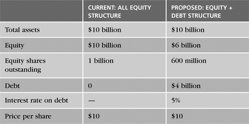
It is important to understand how leverage affects standard metrics of financial performance before we offer a theory about how much leverage a firm should undertake. Consider the example of Creative Financial Concepts, Inc. (CFC). It is an all-equity firm with total assets and a total market value of $10 billion with 1 billion shares outstanding. The market value per share of equity is $10. The firm is evaluating whether it should borrow $4 billion and use the proceeds to repurchase equity. After the repurchase, $6 billion would be left in equity, which implies that 400 million shares ($4 billion/$10) would be repurchased. Thus, this is a “pure” financial decision that is independent of the firm’s investment decisions. The debt carries an interest rate of 5%. Consequently, the firm wants to determine whether the contemplated stock repurchase creates or destroys value for its shareholders. To explore arbitrage in light of M&M, we ignore taxes and bankruptcy costs. Furthermore, note that the price per share of CFC remains the same under either capital structure. We will explore the potential valuation effect of capital structure shifts using arbitrage in a subsequent section. The firm’s capital structure decision is summarized in Table 7.1.

Table 7.1. Creative Financial Concepts, Inc.: Current Versus Proposed Capital Structure

In evaluating the proposed capital structure change, CFC’s management produces the scenario analysis of potential changes in the company’s fortunes shown in Figure 7.1 and Table 7.2. This includes pessimistic, most likely, and optimistic scenarios for earnings before interest (EBI) and the implied returns on assets and equity. It also includes the expected effect of the capital structure changes on earnings per share (EPS) under each scenario. In this context, EBI is a rough proxy for the firm’s cash flow.

Figure 7.1. The Effect of Leverage on Creative Financial Concepts, Inc.

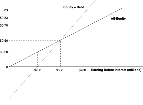
Table 7.2. Creative Financial Concepts, Inc.: Scenario Analysis of Capital Structure Decision

Figure 7.1 shows that the all-equity and combined debt/equity capital structure plans have the same EPS of $0.50 at an EBI level of $500 million. This is a useful reference point in evaluating the trade-off between the two plans’ EPS for projected levels of EBI. Projected EBI in excess of that reference point of $500 million produces a higher EPS under the combined plan than under the all-equity plan. In contrast, projected levels of EBI below the reference point of $500 million have a lower level of EPS under the combined plan than under the all-equity plan. This confirms our intuition that leverage has an advantageous effect on EPS when operating earnings are more than sufficient to cover the associated interest charges, and that leverage will damage EPS when operating earnings are low relative to such interest charges. Figure 7.1 also shows that the slope of the combined plan exceeds that of the all-equity plan. Thus, the rate of change in EPS for a given change in EBI is greater under the levered plan than under the all-equity plan. Noting that variability is the standard measure of risk in finance, the different slopes mean that the levered plan is riskier than the all-equity plan, because it implies higher variability in EPS for a given fluctuation in EBI.

Table 7.2 shows that the return on assets (ROA—earnings before interest/total assets) and the return on equity (ROE—earnings after interest/equity) are equal within each given scenario under the all-equity capital structure. This makes sense, because the all-equity alternative has no debt. Thus, EBI is the same as earnings after interest (EAI). Furthermore, there is no difference between total assets and the equityholders’ investment. However, ROE exceeds ROA when earnings are more than sufficient to service the interest charges under the levered capital structure. In this case, the income from investments outstrips the cost of the associated financing. As expected, in this situation, EPS is higher under the levered case than under the all-equity case. Conversely, in the pessimistic scenario in which earnings can only just cover interest, ROE is less than ROA, and EPS is lower than under the all-equity alternative.

This analysis indicates that the use of leverage at higher projected levels of operating earnings is generally associated with higher EPS. Does this suggest that a firm’s leverage decision always adds value? No. This is like asking why an investor would not always prefer the asset offering the highest expected return. The answer is that higher expected returns are associated with higher risk.

M&M acknowledge this trade-off in Proposition II, which observes that increasing leverage inflates equityholders’ return requirements because leverage increases the risk they bear. This may be generalized to portray the relationship between a firm’s ROA and its ROE, which correspond to the return to a shareholder in an all-equity firm and the return to a shareholder in a levered firm, respectively:

This implies that the return to a levered firm’s owners, as measured by its ROE, exceeds that of an unlevered firm, as measured by its ROA, by the extent to which the unlevered firm’s ROA exceeds the required return on debt (R_D) and as more debt is used relative to equity (D/E) in the capital structure given that ROA exceeds R_D.

Consider the relationship between ROE and ROA using the data in Table 7.2. In the most likely scenario, ROA is 7%, D/E is 0.667 ($4 billion/$6 billion), and R_D is 5%. Thus:

which portrays how the return to the stockholders is altered by the use of financial leverage.

Does the relationship between ROE and ROA make capital structure decisions relevant? No. As a firm adds more debt, it substitutes cheaper debt for increasingly expensive equity in its capital structure such that the overall cost of capital remains the same. Thus, the overall cost of capital is invariant with respect to changes in leverage. Of course, this ignores the benefit afforded by the tax-deductibility of interest charges in most countries and the cost of an increasing probability of bankruptcy as more debt is used in the capital structure. Yet, as noted earlier, M&M purposely sets up a model that simplifies reality so that they can show what matters by first showing what does not. Having shown the measurable effect of using financial leverage, it is possible to show how arbitrage enforces the irrelevance of capital structure decisions in the absence of market imperfections such as corporate income taxes and bankruptcy costs.

Arbitrage and the Irrelevance of Capital Structure

The Essence of Capital Structure Arbitrage Strategy

The irrelevance of capital structure decisions depends on the existence of a strategy that prevents investors in firms that differ only in financial leverage from obtaining different returns at the same risk. Therefore, we’ll now explore whether a strategy exists in which a firm’s leverage can be “undone” by an investor who is willing to adopt the appropriate mixture of debt and equity. If such a strategy exists, an investor will not value two otherwise identical firms differently just because the amount of debt used by each firm differs.

Relying on the framework developed in Chapter 1, “Arbitrage, Hedging, and the Law of One Price,” an arbitrage strategy should earn a riskless profit by taking advantage of different prices for essentially the same firm if the investor can neutralize the effect of different capital structures. In other words, more than the risk-free return can be earned on a riskless position, a situation that is not sustainable.

Arbitrage Strategy for the Example of Creative Financial Concepts, Inc.

Reconsider the firm presented in the earlier example, CFC. An investor wonders if a strategy can be designed to neutralize any valuation effect resulting from CFC’s move from an all-equity structure to the levered capital structure described in Table 7.1. Specifically, he explores the strategy of purchasing the shares of the all-equity firm, partially with borrowed funds, in an effort to replicate the same results as a comparable investment in the levered firm. Thus, he wants to use personal or “homemade” leverage to achieve the same result as that under CFC’s corporate leverage. To do so, he will borrow money personally to the same extent that CFC is considering using leverage. Thus, the investor will mirror the 40% debt, 60% equity capital structure mix described in Table 7.1. Importantly, this strategy is tantamount to considering whether a firm comparable to CFC in every other respect but its leverage would be valued the same by the market.

Our analysis compares the initial investments and payoffs of two strategies: buying shares in CFC under the levered capital structure, and buying shares in CFC under the all-equity capital structure using personal debt in the same proportion as that in CFC’s levered capital structure. If the two strategies require the same initial investment and produce the same payoff profiles, they must be priced equivalently to preclude an arbitrage opportunity. In other words, the different capital structures should be valued the same in the market.

Table 7.3 portrays these two strategies. Strategy 1 buys 1,000 shares of CFC under the levered capital structure at $10 per share for a total investment of $10,000. Strategy 2 buys shares in CFC under the unlevered capital structure such that it also requires the investor to put up only $10,000 of his own money. Consequently, Strategy 2 relies on personal leverage that is consistent with CFC’s corporate leverage of 60% equity and 40% debt to buy 1,667 shares of the unlevered company. The payoffs presented under the three scenarios are based on the EPS outcomes for the all-equity and levered capital structures described in Table 7.2. The EPS outcomes are adjusted by the number of shares held in each respective strategy to produce the indicated payoffs under each scenario. Furthermore, in Strategy 2, the interest paid on the personal debt is deducted to produce the net payoff under each scenario.⁴

Table 7.3. Arbitrage Strategy for Creative Financial Concepts, Inc.: Corporate Versus Personal Leverage

Strikingly, Table 7.3 shows that the net payoffs across each scenario are the same for both strategies. Furthermore, by construction, the initial investment for each strategy is the same at $10,000. If the initial investments and net payoffs produced by the two strategies are identical, they should be priced identically under the Law of One Price, introduced in Chapter 1. Thus, CFC’s capital structure decision is irrelevant to the valuation of its equity. In terms of M&M’s Proposition I, the values of the unlevered firm and the levered firm are the same.

Arbitrage of Misvalued Capital Structure

As the previous chapters have shown, in arbitrage-based arguments, the exception proves the rule. Prices are sustainable only when they preclude arbitrage because violations create riskless opportunities to earn more than the risk-free return. And so it is with two otherwise-comparable firms that differ only in their capital structures and yet are valued differently in the market.

Reconsider the preceding example of CFC. The total value of the firm’s assets under the all-equity capital structure is $10 billion. The firm under the levered capital structure is financed with $6 billion in equity and $4 billion in debt. What if the value of CFC’s equity was greater under the levered plan than under the unlevered plan? Assume that the value under the levered plan is $12 per share and the value under the unlevered plan is $10 per share. Revisiting the preceding two strategies, it would now be more expensive to set up Strategy 1 than Strategy 2. However, the two strategies would still produce the same net payoffs. Consequently, this would imply that the same asset is effectively selling for two different prices. This creates an incentive for investors to pursue Strategy 2, in which shares in the unlevered CFC are purchased using some borrowed money. Investors would not buy shares in the levered firm because the return (net payoff) can always be obtained more cheaply through Strategy 2. This would put downward pressure on the levered firm’s share price until it was equal to that of the unlevered firm’s equity. Investors could earn an arbitrage profit by selling short shares in the levered firm and using the proceeds to buy shares in the unlevered firm in part with borrowed funds.

The Reality of Capital Structure Arbitrage

The preceding arbitrage argument assumes that individual investors can borrow at the same rate as corporations. This raises the question of whether individuals may really only be able to borrow at higher rates. If firms can generally borrow at lower rates than individuals, does corporate leverage add value? Although this is plausible in theory, there is ample reason to believe that individuals can borrow at rates not too much higher than the risk-free rate in practice. Thus, individuals can be expected to borrow at rates that compare favorably with the rates at which firms borrow.

Consider how the average individual investor often borrows money to buy stock—by borrowing money from his or her broker. Under current U.S. initial margin regulations, an investor must put up a significant amount of a stock’s purchase price.⁵ Furthermore, investors must maintain a margin over the life of the investment, which is usually in the range of 25% to 30%. And the stock is usually pledged as collateral for the loan. Thus, brokers face little risk on such loans and consequently charge a rate that is not much higher than the risk-free rate.

In contrast to individual investors, most corporations borrow money by pledging physical assets, such as long-term equipment, as collateral. Such assets are far less liquid than stocks. Thus, when corporate borrowers default, it is typically harder for lenders to get back all their money than when individual investors default on brokers’ loans. Consequently, it is reasonable to expect individual investors to face comparable or lower loan rates than corporations. Thus, the capital structure argument does not break down due to significant differences between corporate and individual borrowing rates.

Although the preceding M&M analysis suggests that capital structure decisions are irrelevant to a firm’s valuation, the analysis does not stop there. As previously discussed, the initial M&M model assumes that there are no taxes or bankruptcy costs. The tax-deductibility of interest in the U.S. is a benefit of leverage because the government effectively subsidizes the use of debt, thereby reducing its cost. Furthermore, increased reliance on debt implies a higher probability of bankruptcy, which is costly. Thus, the initial M&M model uses arbitrage to show that capital structure decisions are irrelevant in the absence of the discussed costs and benefits. It is unsurprising that such decisions are irrelevant when the analytical model recognizes neither costs nor benefits. Subsequent analysis by M&M selectively adds the benefit afforded by the tax deductibility of interest without considering bankruptcy costs.⁶ As expected, this makes the capital structure decision completely relevant in the sense that the optimal capital structure is all-debt. This is because debt is presented as having only benefits and no costs.

Ultimately, theory and practice are reconciled by recognizing that an optimal capital structure balances the benefits of the tax deductibility of interest with the costs of potential bankruptcy.⁷ Furthermore, capital structure relevance can result from the market’s drawing inferences about the “signal” that better-informed managers are effectively sending to less-informed investors through their capital structure decisions. Notwithstanding these interesting extensions of capital structure theory, M&M’s analysis introduced arbitrage into modern financial analysis in a path-breaking way.

Options, Put-Call Parity, and Valuing the Firm

Viewing the Firm as a Call Option

Capital structure analysis embraces the different perspectives of bondholders and equityholders in valuing a firm. While it makes sense for their perspectives to differ, it is also reasonable to expect a common link between their valuations. This section considers firm valuation from each perspective using the analogies of European calls and puts. The links between the two perspectives also are explored using the put-call parity framework developed in Chapter 5.

Again, consider the example of CFC, which recall is financed with $4 billion in bonds and $6 billion in equity under its levered plan. Examine the admittedly artificial but nonetheless instructive case in which the firm is about to be liquidated. Equity can be viewed as a call option on the firm’s assets. This is because the value received by equityholders depends on whether the value of the firm’s assets is sufficient to pay off the bonds. If the firm’s assets are not worth enough to pay off the $4 billion owed to bondholders, all the assets go to the bondholders, and the equityholders end up with no residual value. Alternatively, if the firm’s assets are worth more than $4 billion, bondholders are paid in full, and the residual is left to the equityholders. In essence, the bondholders own the firm’s underlying assets and may be viewed as having written a call option on the firm’s assets with an exercise price equal to the amount of debt. This is like a covered call strategy.

Figure 7.2 portrays the value of a firm as a call option from the perspectives of the stockholder and bondholder. The exercise price of the implicit call option, X, is the face value of the firm’s debt, which is $4 billion in this example. The top diagram in Figure 7.2 shows that equityholders may be viewed as long the call option on the firm’s assets. The bottom part shows that bondholders may be viewed as having written the call option on the firm’s assets. Each call has an exercise price equal to the debt’s face value (X = $4 billion). Thus, the bondholders own the firm’s underlying assets and have written a covered call on those assets.

Figure 7.2. Viewing the Firm as a Call Option

Stockholders will exercise their effective call options if the firm’s value exceeds X = $4 billion. They will not exercise their option if the firm’s value is less than X = $4 billion. For example, if the firm’s value is $6 billion, stockholders will exercise their right to effectively buy the firm from the bondholders for the value of the debt at $4 billion and will pocket the $2 billion difference. Conversely, if the firm’s value is only $3 billion, stockholders will not exercise their option and will sacrifice all the firm’s remaining value to the bondholders, who receive the $3 billion in payment for the outstanding debt. In summary, stockholders may be viewed as holding a call option on the firm’s assets, and bondholders may be viewed as having sold such a call option.

Viewing the Firm as a Put Option

Put-call parity shows that there is a relationship between puts and calls on the same underlying asset. Therefore, it should be possible to recast the preceding analysis of a firm’s value in terms of puts rather than just in terms of calls. Again, it is important to distinguish the perspectives of stockholders and bondholders.

Stockholders are viewed as owning the firm’s assets, which have been financed with debt that is to be paid back to bondholders. Furthermore, stockholders may be viewed as holding a put option that allows them to sell the firm to the bondholders for an exercise price equal to the debt’s value (X = $4 billion). Stockholders would exercise the right to sell the firm for the exercise price if the firm’s value is less than X = $4 billion. Rather than actually receiving the $4 billion payment, this would offset the $4 billion debt that stockholders owe the bondholders. Thus, the net payoff to stockholders in this case is zero. Alternatively, if the firm’s value exceeds the exercise price, stockholders have no incentive to exercise their put on the firm and simply pay the bondholders what they are owed—$4 billion—and retain the rest of the assets.

If stockholders may be viewed as holding a put option on the firm, bondholders may be viewed as having sold that put on the firm to stockholders. If the firm’s value is less than X = $4 billion, stockholders exercise their put, and bondholders surrender their claim to be paid the debt of $4 billion. This is because surrendering the claim offsets their obligation to pay the exercise price of $4 billion on the “in-the-money” put on the firm. The bondholders’ net payoff in this case is zero. Conversely, if the firm’s value is greater than X = $4 billion, stockholders do not exercise their put, and bondholders are paid the $4 billion debt owed them.

Integrating the Call and Put Perspectives with Put-Call Parity

The preceding analysis shows that equityholders may be viewed as holding a call option on the firm’s assets, and bondholders may be viewed as having sold that call to equityholders. Equityholders may also be viewed as holding a long put on the firm’s assets, which bondholders have sold to them. While clear enough in context, the discussion still begs the question of how these two distinct perspectives may be reconciled. In other words, while the put and call perspectives make sense individually, do they also make sense when considered jointly? Put-call parity reconciles these two ways of interpreting equity and bond investments in the firm.⁹

Recall the put-call parity framework developed in Chapter 5 for European options on non-dividend-paying stocks. By way of brief review, we considered a call option with a price of C and a put option with a price of P, both on the same underlying stock with a current price of S₀. The options have the same exercise price X and the same expiration date T, which is CFC’s planned liquidation date. U.S. T-bills with a face value of X, maturing at the same time the options expire, yield R_f percent. S_T is the value of the stock on the expiration date. In the current context, X is the face value of the bonds used to finance the firm. The market value of the bonds today is B₀. Put-call parity for European options is:

S₀ + P = C + X/(1 + R_f)^T

The framework portrays the relationship between call and put prices, the underlying stock price, the exercise price, the risk-free rate, and the time to expiration. Keep in mind that the relationship considers only risk-free debt. Put-call parity can be used to relate the stockholder and bondholder perspectives to each other in light of the call and put positions.

Recast the stockholders’ position in terms of put-call parity. Consider their position as long call holders:

C = S₀ + P – X/(1 + R_f)^T

Restate this in light of the fact that the underlying position for the options is the firm’s assets, A₀:

C = A₀ + P – X/(1 + R_f)^T

This relates the call and put perspectives to one another from the stockholders’ vantage point. The left side presents the call perspective, and the right side presents the put perspective. The stockholder is effectively long both calls and puts on the firm’s assets. The value of a call on the firm’s assets is equal to the value of the firm’s assets (A₀), less the value of the debt (X/(1 + R_f)^T), plus the value of the put (P) that allows stockholders to effectively give, or put, the firm’s assets to bondholders to satisfy their debt. This is consistent with the intuition that the value of the shareholders’ position is positively related to the firm’s value, is negatively related to the amount of debt carried by the firm, and is enhanced by the presence of the put option.

Examine the bondholders’ position in terms of put-call parity. Recall that bondholders are effectively short both call and put options on the firm’s assets. Thus, it is helpful to rearrange put-call parity to express these positions jointly:

S₀ – C = X/(1 + R_f)^T – P

This can be restated as before to capture that the underlying position in this context is the value of the firm’s assets, A₀:

A₀ – C = X/(1 + R_f)^T – P

Thus, the left side shows that bondholders are short the call, and the right side shows that they are also short the put. The signs of the indicated components are consistent with intuition. Bondholders’ fortunes improve as the value of the firm’s assets increases and as the value of the debt increases. In contrast, the value of their position is eroded by increases in the values of either the calls or the puts they have sold to stockholders.

The value of the bonds issued by the firm has not been explicitly identified because put-call parity considers only risk-free, pure-discount debt. The firm’s assets are financed using both debt and equity. Thus:

A₀ = S₀ + B₀

Reconsider put-call parity, expressing the stockholder’s position as a call on the firm’s assets. Thus, restating put-call parity to solve for the call price, we substitute S₀ for C on the left side and A₀ for S₀ on the right side:

S₀ = A₀ + P – X/(1 + R_f)^T

Consequently, the value of the firm’s debt can be inferred as:

B₀ = A₀ – S₀ = X/(1 + R_f)^T – P

This implies that the value of a firm’s risky debt is equal to the value of a riskless bond and a short put, which bondholders have sold to equityholders. This makes sense in light of the observation that the stockholders’ position is a claim to the firm’s assets, a long put, minus the value of a risk-free bond: S₀ = A₀ + P – X/(1 + R_f)^T. This completes the portrayal of firm valuation from the perspectives of stockholders and bondholders in light of their implicit option positions.

Summary

This chapter explained the role of arbitrage in assessing the relevance of capital structure decisions in the context of the Nobel Prize-winning Modigliani-Miller (M&M) theory. The chapter also showed how the firm may be viewed as put and call options and used the put-call parity framework to explain how a firm is valued from the distinct though linked perspectives of bondholders and stockholders.

M&M’s Proposition I demonstrates that a firm cannot change the total value of its securities just by splitting cash flow claims into different streams. In contrast, a firm’s value is determined by its real assets, not by the financial assets it issues against those real assets. The chapter presented the common analogy of pizza: cutting an extra-large pizza into eight rather than six pieces does not increase the amount of pizza you can eat for dinner. By implication, no matter how you distribute financial claims to the firm sold in the capital markets, the real assets that determine the firm’s value remain the same. Arbitrage ensures that the cost of capital is invariant to capital structure decisions.

To provide a frame of reference for capital structure arbitrage analysis, this chapter discussed how the effects of financial leverage are measured. Ultimately, it may be generalized that the use of leverage at higher projected levels of operating earnings is associated with higher EPS. Yet this does not necessarily imply that a firm’s leverage decision adds value. This is because leverage brings greater risks as well as greater potential returns. Indeed, M&M acknowledge this risk/return trade-off in their Proposition II:

As discussed in this chapter, this proposition implies that the return to a levered firm’s stockholders, as measured by its ROE, exceeds that of an unlevered firm, as measured by its ROA, by the extent to which the unlevered firm’s ROA exceeds the required return on debt R_D and as more debt is used relative to equity (D/E) in the capital structure.

After measuring the effect of financial leverage, this chapter explained that the irrelevance of capital structure decisions depends on investors’ ability to “undo” a firm’s corporate leverage using a strategy that involves personal borrowing. The analysis showed that investors can successfully do so. Thus, M&M’s Proposition I is upheld because the values of the unlevered firm and the levered firm are the same.

This chapter showed that equityholders may be viewed as holding a call option on the firm’s assets and bondholders may be viewed as short that call. Furthermore, equityholders may be viewed as holding a long put on the firm’s assets, which bondholders have sold to them. Put-call parity is used to reconcile these two ways of interpreting equity and bond investments in the firm.

Under the assumption that the underlying position is the firm’s assets, put-call parity relates the call and put perspectives to one another from the stockholders’ viewpoint as:

C = A₀ + P – X/(1 + R_f)^T

As discussed in this chapter, the left side presents the call perspective, and the right side presents the put perspective. The stockholder is effectively long both calls and puts on the firm’s assets. More specifically, the value of a call on the firm’s assets is equal to the value of the firm’s assets (A₀) less the value of the debt (X/(1 + R_f)^T) plus the value of the put (P) that allows stockholders to sell the firm’s assets to bondholders to satisfy their debt.

Similarly, bondholders are effectively short both call and put options on the firm’s assets such that:

A₀ – C = X/(1 + R_f)^T – P

Thus, the left side shows that bondholders are short the call, and the right side shows that they are also short the put.

This chapter concluded by observing that the value of a firm’s risky debt can be portrayed using put-call parity as:

B₀ = A₀ – S₀ = X/(1 + R_f)^T – P

This affords the insight that the value of a firm’s risky debt is equal to the value of a riskless bond and a short put, which bondholders have sold to equityholders.

Endnotes

¹ Miller (1999, p. 100).

² Modigliani and Miller (1958). While M&M’s analysis is also applied to dividend policy, the current discussion is limited to capital structure, because it lays bare the essentials of their arbitrage-based arguments.

³ Myers (1999, p. 206).

⁴ For simplicity, it is assumed that the investor can borrow at the same interest rate as the firm. This assumption is evaluated next.

⁵ Current regulations require an initial margin of 50%, which is applied on a portfolio basis rather than on an individual investment basis.

⁶ Modigliani and Miller (1963).

⁷ Excellent discussions of corporate capital structure theory and practice may be found in Ross, Westerfield, and Jaffe (1999, Chapters 15 and 16) and Brealey, Myers, and Allen (2006, Chapters 17–19).

⁸ Calamos (2003, pp. 218-219). See Currie and Morris (2002) for an interesting overview of capital structure arbitrage.

⁹ See Rous, Westfield, and Jaffe (1999, p. 566-570).