CHAPTER 15
Inventory and Warehouse Management

Planning, replenishing, consuming, and shipping inventory in an optimal manner can save millions by reducing obsolescence and increasing the inventory turns. These business processes consume a lot of labor and equipment to store, retrieve, and move these materials. For example, to move a pallet, you may need a pallet jack or a fork truck and a employee who is trained to work with that equipment. To pick peaches, you might just need a peach picker and no specific equipment. Using these resources in an optimal manner is a very important objective for warehouse managers. Figure 15-1 shows the different types of material transactions that take place in a warehouse.

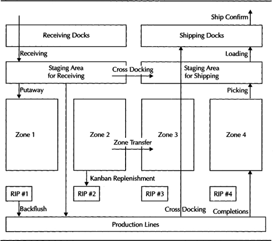
FIGURE 15-1. Material handling tasks in a warehouse/manufacturing plant

This chapter discusses the features provided by Oracle Applications to manage the material handling function in a manufacturing plant/distribution center. Most of these features are provided in Oracle Inventory and Oracle Warehouse Management (OWM).

Units of Measure (UOM)

Unit of measure (UOM) is used for all material transactions. UOM Classes define the high-level groupings of UOMs. The grouping is based on the nature of measuring. For example, you can have a class called Quantity that can have UOMs such as each, dozen, and so on. Another class could be weight, with lb, kg, and ton as UOMs. Each class contains one base UOM.

You can define conversions between UOMs. Standard conversions define conversions that are not specific to the item or the class. A dozen equals 12 each is a standard conversion. Item-specific conversions identify the relationship between two UOMs, with respect to an item. For example, you can put 12 EA of item X in the case BigBox. But, you might be able to put 24 EA of item Y in the same case.

The on-hand balance (covered in the section “On-Hand Balances”) for each item is maintained in the primary UOM of the item, which is identified using the item attribute Primary UOM. You must define a conversion between a non-base unit of measure and the base unit of measure before you can assign the non-base unit of measure to an item.

When you define an item, you decide which type of unit-of-measure conversion to use—item-specific, standard, or both. If you specify item-specific, the system uses unit of measure conversions unique to this item. If none exist, you can transact this item in its primary unit of measure only. If you specify Standard, standard UOM conversions are used. If you specify Both, both item-specific and standard unit of measure conversions are considered. If both exist for the same unit of measure and item combination, the item-specific conversion is used. Unless you have a specific reason to exclude either standard or item-specific conversions, the system default of Both is almost always an appropriate choice.

NOTE
UOM definitions are stored in the table MTL_UNITS_OF_MEASURE. All the conversions are stored in the table MTL_UOM_CONVERSIONS.

During transaction execution, when you enter an item’s quantity, the default is the primary unit of measure for the item. You can select a UOM that has either the standard or item-specific conversions from the primary unit of measure. Transactions are performed in the unit of measure you specify. The conversion happens automatically, and item quantities are updated in the primary unit of measure of the item.

Material Transactions

Material transaction is a general term that represents material movement in a warehouse or a manufacturing plant. For example, when you move material between zones or release material to the shop floor for production, you are performing a material transaction.

Material transactions have two aspects: change of physical location and the impact to material accounts. The two concurrent programs—Transaction Manager and Costing Manager—are responsible for processing these two aspects of each material transaction. You can also process your transactions online, instead of using the Transaction Manager.

Transaction Source Types

The transaction source type represents the type of entity in Oracle Applications that a transaction can originate from. For example, the source type of a PO Receipt transaction is a purchase order. A number of transaction source types are seeded as system-defined transaction source types. Additionally, you can define source types if you need to validate your transactions against a different type of entity. The User-Defined tab in the Transaction Source Types form allows you to do that. You can select the Validation Type as None or Value Set. If you want to validate against a dynamic list of values, you can define a SQL query-based value set if you want.

Transaction Actions

The transaction action identifies the nature of material movement. It is generic and not specific to any source. For example, the action Receipt Into Stores just means that some material is going to be received into inventory. With the transaction source type of Purchase Order, this action indicates a PO Receipt; with the transaction source type of an Account, this action indicates an Account Receipt. Oracle Applications comes seeded with many transaction actions.

Transaction Types

Transaction type represents a convenient way of representing a transaction source type and transaction action and offers a classification mechanism for classifying your transactions by using meaningful names.

In some cases, transactions happen behind the scenes—as it does with sales order issue, for example. When you ship an item, the sales order issue transaction happens behind the scenes. In certain other cases, you are allowed to specify the transaction types. For example, when you perform a miscellaneous receipt or a WIP completion, you are allowed to specify the transaction type you want to use. Based on this, you are allowed to define transaction types that include a subset of transaction source types and transaction actions. For example, you cannot use Sales Order as the source type for the transaction types that you define. But, you can use the transaction source type Inventory in your transaction types.

Transaction types that have actions—such as Receipt Into Stores, In-Transit Receipt, Direct Organization Transfer, Assembly Completion, or Negative Component Issue—allow you to specify whether you want to receive Shortage Alerts when those transactions happen. Shortage alerts communicate the receiver of any material shortage in some usage point.

Transaction Reasons and Corrective Actions

While performing an inventory transaction, you can choose a transaction reason to classify the transaction. From an OWM perspective, transaction reasons serve two purposes: identifying the reason for not performing the directed task and automatically initiate a corrective action. When a user is not able to complete a directed task, the user will be prompted to enter a reason. Based on the selected reason, the associated workflow will be launched. For example, if a picker cannot perform the task due to inadequate quantity in the suggested locator, the actions could be to generate a cycle count automatically, perform the adjustments, and then notify the warehouse manager about this discrepancy.

You define transaction reasons in the Transaction Reasons form. When you define a reason, you identify the reason type, which is used to restrict the reason list for each task type. For example, a reason type that you define for picking cannot be used during problems in putaway. You can optionally associate a workflow that will be launched when the associated reason is selected.

Cost Groups

In the pre-11 i releases (and the 11 i installations that don’t enable OWM), subinventory is both a physical zone and a logical collection of accounts that tracked the value of the items in the subinventory.

When you install OWM, a subinventory is purely a physical zone. The logical collection of accounts is separated from subinventory and is provided using cost groups. To provide backward compatibility, the subinventory form will accept a cost group as the default cost group for the subinventory and the Accounts tab in the subinventory form will display the accounts in the cost group. The accounts in the subinventory form cannot be edited directly, although you can change the default cost group for the subinventory.

NOTE
Even in the installations where you don’t enable OWM, a cost group is automatically defined in the name of the subinventory, with the subinventory accounts; the underlying cost group is used in the transactions behind the scenes.

You define cost groups in the Cost Groups form. The Cost Groups form allows you to define the various valuation accounts and variance accounts that are needed to handle standard costing, average costing, FIFO costing and LIFO costing. A complete coverage of these costing methods is dedicated to Chapter 18.

If you don’t have OWM, you provide the subinventories and locators that are involved in the transaction; the system will determine the cost group from the subinventory or organization settings. OWM provides you with a rules framework that can automatically determine the cost group for a transaction based on numerous criteria. The rules engine will use only the default cost group at the organization level if it is not able to find a cost group. Cost Group rules are covered in the section “The Rules Framework”.

OWM also provides transactions to change cost group, independent of physical movement.

Material Status Control

When you find material discrepancies in a zone, you may want to prevent all new transactions from and to this zone and perform an emergency cycle count. The Material Status Control feature allows you to do exactly this and helps you in managing similar situations with locators, lots, and serials.

You define material statuses in the Material Status Definition form shown in Figure 15-2. The status usage identifies to which entities this status can be applied. For example, you might want to apply a status to a subinventory to prevent the receiving transactions into the subinventory and not intend to use it for lots.

FIGURE 15-2. The Material Status Definition form allows you to identify the allowed and disallowed transactions for each status

The Transactions Shuttle Region lists the allowed transactions and disallowed transactions in two text lists. You can move the listed transactions between these two lists using the Shuttle Control that is provided between the two text lists. When a status is applied to an entity, entity will be prevented from all the disallowed transactions. For example, if you find that a particular lot contained defective components, you can define a status called Hold that disallows all the transactions and apply that status to the lot in order to prevent that lot from being shipped or used in manufacturing. Once you segregate the defective pieces, you can change the status of the lot back to Normal.

NOTE
An item in inventory might get its status from the serial and lot to which it belongs and the locator and subinventory in which it currently resides. The transactions that are disallowed by these statuses will not be allowed for this item; it is a cumulative effect. For instance, consider a lot packed into an LPN. This LPN may contain other items packed into it that are not status controlled. If the lot packed into this LPN is assigned a status that prevents customer shipments, the shipment of the LPN to a customer will be prevented as the system applies a cumulative status while performing a transaction. You can enable lot and serial statuses for items using the item attributes Lot Status Enabled and Serial Status Enabled. In each case, you have to provide a default status.

Executing Transactions

Oracle Applications provides a number of ways to execute material transactions. Depending on the transaction type, transactions need to be executed using different forms. You can execute all transactions either using the desktop or mobile applications.

NOTE
The profile option INV:Transaction Date Validation allows you to decide whether you want to allow transaction dates to be a past date or a date in the past period.

Subinventory Transfers

You can execute subinventory transfers from the Subinventory Transfers form. The transaction results in the movement of material between two locations within an organization. The locations can be either subinventories or locators.

NOTE
The profile option INV:Allow Expense To Asset Transaction allows you to decide whether you want to allow transferring material from an expense subinventory into an asset subinventory.

Miscellaneous Transactions

Miscellaneous transactions are a way of issuing material to or receiving material from groups that are not inventory, receiving, or work in process, such as a research and development group or an accounting department. With a miscellaneous transaction you can issue material to or receive material from General Ledger accounts.

You can use your user-defined transaction types and sources to further classify and name your transactions. You can perform the receipts for items that were acquired by means other than a purchase order from a supplier. Miscellaneous transactions are very handy during the initial implementation phase for testing various transaction scenarios.

NOTE
The Material Workbench (covered in this chapter) allows you to perform mass move and mass issue transactions where you can move all the material in a zone in one transaction.

Inter-Organization Transfers

Interorganization transfers allow you to transfer material between inventory organizations. The transaction is available in two shipment modes: direct or intransit shipments. You can use a single transaction to transfer more than one item. The items you transfer must exist in both organizations, although they can have different attributes and control level (locator, revision, lot, and serial number) settings. You perform interorganization transfers on the Interorganization Transfer form. The transfer type, in-transit ownership, in-transit accounts, and other details are defined on the Shipping Network Between the Two Organizations. Shipping networks are covered in Chapter 2.

Direct Shipment

Direct shipment results in the movement of materials to the destination organization immediately. The source and destination information are required at the time of the transaction. You cannot perform a direct transfer of items that are not under revision/lot/serial number control in the shipping organization if the destination organization requires any of these controls. For example, if an item is under revision control in organization A01, you cannot ship the item from organization A02 to A01 if the item is not under revision control in A02.

In-Transit Shipment

In-transit shipment is typically used when transportation time is significant or if you require separate shipping and receiving steps. The delivery location need not be specified at the time of the transfer transaction. Only the source and freight information is required. The interorganization transfer charge is specified when the shipping network was defined between the two organizations. Based on the interorganization transfer charge that applies between the organizations, a percentage of the transaction value or an absolute amount is used to compute transfer charges.

If the FOB point is set to Receipt in the shipping network, the destination organization owns the shipment after receiving the items. If it is set to Shipment, the destination organization owns the shipment when the shipping organization ships it and while it is in-transit. You can update the freight carrier or arrival date in the Maintain Shipments window.

At the time of shipment, the receiving parameters for the destination organization should have been defined. You can receive and deliver your shipment in a single transaction or receive and store your shipment at the receiving dock. Receiving was covered in detail in Chapter 14.

You can perform an in-transit shipment of items that are not under revision/lot/serial number control in the shipping organization even if the destination organization requires any of these controls. In the case of lot- and serial-number-controlled items, you will be required to provide a value during receiving. In the case of revision-controlled items, you can receive only the same revision that was shipped.

Move Orders

A move order is a mechanism for requesting, sourcing, and transferring materials within an organization. Move orders also allow you to track the movement of material within a single organization. They allow materials managers/planners to request and authorize the movement of material within a warehouse for purposes such as putaway, replenishment, and picking. You can generate move orders either manually or automatically depending on the source type you use. All the move orders created are automatically preapproved.

Subinventory Transfer Move Order Requisition

A subinventory transfer move order requisition and a regular subinventory transfer achieve the same end result: transferring material between subinventories or locators. However, the processes have significant differences, as highlighted in Table 15-1. Both subinventory transfer and move order are useful in different circumstances, and you should establish procedural control on using these two methods of transferring material between subinventories.

TABLE 15-1. Comparing Move Order Requisitions with Subinventory Transfer

Pick Wave Move Order

A specific type of move order called the Pick Wave Move Order is used for managing the outbound logistics of the pick released materials. Wave picking is discussed in the section “Wave Picking”, Pick wave move orders are automatically created by releasing sales order lines for picking, as described in Chapter 17.

Replenishment Move Order

The planning processes, such as Min-Max planning and ROP planning, and the replenishment processes, such as replenishment counting and intra-org kanban can automatically create preapproved move orders of type replenishment. (Kanban is discussed in the “Kanban Materials Management” section later in this chapter.)

Pick Releasing WIP Requirements

Starting from Release 11 i.6, you can pick release WIP requirements: requirements of discrete jobs, repetitive schedules, and flow schedules. If you use backflushing, the picked materials will be directed to the backflush subinventory and locator. If you intend to issue the material to the job/schedule, the appropriate WIP job/schedule will be indicated to the picker.

Creating and Using Move Orders

You create move orders in the move orders form. The header contains the move order number and description. Each line indicates a material requirement. The line contains the required item, quantity, and the destination details. You can optionally specify source information.

Once you submit the move order for approval, the item planner (specified by the item attribute Planner in the General Planning tab) for each line gets notified. When the planner approves the move order line, the move order line becomes eligible for transaction.

The Transact Move Order Lines form allows you to perform detailing and move order transactions. If the source information is not complete, you can click the Location Details button to request the system to suggest sourcing suggestions. This process is called detailing—it creates a pending reservation that will be consumed when you transact the line. It therefore decrements the available-to-transact (ATT) quantity.

The profile option INV:Detail Serial Numbers allows you to specify whether you want the detailing process to suggest individual serial numbers. When this profile option is turned on, each pick task asks the picker to pick individual serial numbers, which results in the picker searching for the serialized item. In most cases, you save a lot of time by turning this profile option off. When the profile is turned off, you can pick the items in whatever order you want and enter the serial numbers as you pick.

By clicking the Transact button, you can transact the move order lines that have been detailed.

Material Workbench

The Material Workbench provides a convenient user interface for performing the common material transactions. It also provides the ability to perform various queries such as availability. Figure 15-3 shows the Material Workbench. The tree navigator on the left pane allows you to navigate among the different warehouses and drill down to the various zones and locators within each warehouse.

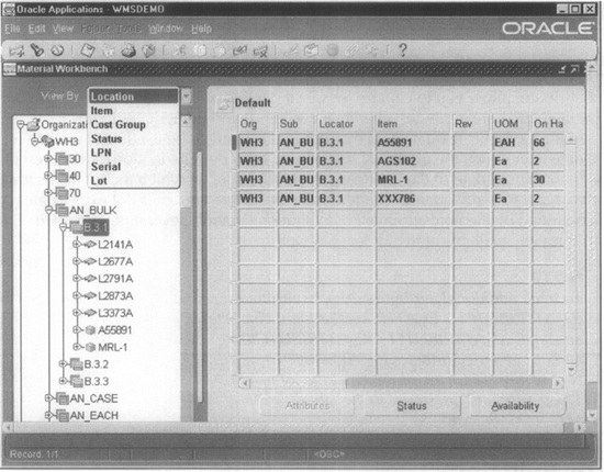
FIGURE 15-3. The Material Workbench allows you to perform mass moves and issues

The Material Workbench supports the Mass Move and Mass Issue transactions from the Tools menu. An example of a mass move transaction is to move all the items in a locator to a different locator. An example of a mass issue transaction is to issue all the items in a locator to an account alias, if, for example, the locator and all its contents were damaged.

In a future release of 11 i, you can create location-based cycle counts from the Material Workbench. You can select a range of locators and schedule cycle count for the selected locators. You can also perform mass updates of statuses.

Movement Statistics

Movement statistics provides the capability for gathering, reviewing, and reporting statistical information associated with material movements in the enterprise. Movement statistics is an important part of the Intrastat reporting requirements of the European Union, which requires tracking material movements regardless of the countries involved in the material movement process.

NOTE
When you perform interorganization transfers, RMA receipts, RMA returns, supplier receipts, and supplier returns, you can invoke the Movement Statistics window from the Tools menu.

Managing Lots

Lots represent a group of on-hand items that generally have the same characteristics. For example, you can classify all the output from a production batch into three lots—each with a concentration of 90 percent, 80 percent, and 70 percent, respectively. The lot functionality in Oracle Applications supports lot attributes, lot splitting, and lot merging. For directed picking or putaway, you can use lot attributes as criteria in your rules.

You can use the material status at the lot level to put the lot on hold for certain types of transactions. For example, you can prevent sales order shipments on a particular lot.

Lot Attributes

Lot attributes allow you to capture lot specific information. The attributes have been classified into date attributes, character attributes, and numeric attributes.

Maturity date is the date a lot matures and is ready to be used. Best by date is the date after which the quality of the lot may degrade. Origination date represents the manufacture date of the lot. Retest date is the date on which the lot needs to be tested again to verify quality. In addition to these date attributes, lot expiry date is controlled by the item attribute Lot Expiration Control. Several other named attributes are available at the lot level as well.

NOTE
To track additional attributes, 20 date attributes (D_ATTRIBUTE1 .. D_ATTRIBUTE20,) 20 character attributes (C_ATTRIBUTE1 .. C_ATTRIBUTE20,) and 30 numeric attributes (N_ATTRIBUTE1 .. N_ATTRIBUTE30) are provided at the lot level. These attributes are stored in the table MTL_LOT_NUMBERS.

Lot Splitting

Lot splitting allows you to split a quantity of material that is produced in a single lot into multiple lots. Splitting may also be performed when a portion of a lot has different characteristics. Lot splitting can be of two types—full and partial lot splits. A full lot split is to split the entire quantity of a lot into new child lots, leaving the parent lot with no quantity. A partial lot split is to split a partial quantity of a lot into new child lots, leaving a remainder quantity in the parent lot. You enable an item for lot splitting using the item attribute Lot Split Enabled. During the lot-splitting process, the lot attributes of parent lot are defaulted to all the child lots. You can perform lot splitting by using the mobile transaction form Lot Split.

NOTE
Parent lot and starting lot mean the same thing, as do child lot and resulting lot.

Lot Merging

Lot merging allows you to merge multiple existing lots into a new lot as well as to merge multiple existing lots into an existing lot. Merging may be performed when you want to store lots together from multiple inventory locations or when the identity of each lot needs not be maintained.

Lot merging supports full and partial lot merges. A full lot merge is to merge the entire quantity of one or more lots into a new lot or an existing lot. A partial lot merge is to merge a partial quantity of one or more lots into a new lot or an existing lot, leaving a remainder quantity in the parent lots.

You enable an item for lot merging using the item attribute Lot Merge Enabled. During the lot merging process, the lot attributes of the resulting lot are defaulted from the starting lot with the largest quantity. If equal quantity lots are merged, the lot attributes will be defaulted from the first specified starting lot. You can merge lots using the mobile transaction form Lot Merge.

NOTE
Merging lots with different cost groups causes problems due to co-mingling. So, for a lot merge, the cost group of all starting lots must be the same.

A lot that has been reserved to a demand cannot be split or merged. Reservation is covered in the section “On-Hand Balances”.

Lot Genealogy

When you split a lot to form multiple sublots or when you merge multiple lots into a single lot, Oracle keeps track of these transactions. Lot Genealogy stores the relationship between lots and sublots. The Lot Genealogy form that is shown in Figure 15-4 provides a tree navigator that you can use to navigate between lots and sublots.

FIGURE 15-4. The Lot Genealogy form allows you to view the composition of a lot and the related transactions

The Job Lot Composition form allows you to view the component lot information for a discrete job. This form is covered in Chapter 16.

The profile option INV:Genealogy Prefix Or Suffix determines how the item number should be displayed along with the lot number in the genealogy tree structure. The two possible settings are Prefix (the lot number is displayed before the item number), and Suffix (the lot number is displayed after the item number). The profile option INV:Genealogy Delimiter determines what should be the delimiter between the item number and lot number.

CAUTION
Without setting the two profiles discussed in the previous paragraph, when the user views the lot genealogy, it will show NULL on the tree node instead of the lot number.

Managing Serialized Items

You can use the serial number functionality provided by Oracle in a variety of situations. At a very high level, serial numbers provide you with the ability to track individual items. Additionally, if you want to track the characteristics or change in characteristics of each serialized item, you can use serial attributes. When you build items in manufacturing, you may want to keep track of the As Built configuration of the serialized assembly and all the serialized components. You can use serial genealogy to keep track of As Built configurations.

Serial Attributes

At the serial number level, you can capture the origination date and country of origin. A number of standard attributes allow you to track the life of the serialized item. For example, cycles Since New allows you to track the number of usage cycles this item has gone through from the beginning of its life. Like lots, serial numbers are also provided with 20 date attributes, 20 character attributes, and 30 numeric attributes for tracking additional attributes. Several other named attributes are available at the serial level as well.

NOTE
To track additional attributes, 20 date attributes (D_ATTRIBUTE1 .. D_ATTRIBUTE20,) 20 character attributes (C_ATTRIBUTE1 .. C_ATTRIBUTE20,) and 30 numeric attributes (N_ATTRIBUTE1 .. N_ATTRIBUTE30) are provided at the serial level. These attributes are stored in the table MTL_SERIAL_NUMBERS.

Serial Genealogy

In certain industries, knowing the As Built configuration of an item is important. The As Built configuration is a multilevel structure that consists of the various lot/serialized components of a serialized assembly. Keeping a record of the As Built configuration allows you to serve your customers better. For example, you can send them periodic reminders for maintaining certain parts. You can also use serial genealogy to investigate customer claims. For example, assume that your customer replaces one of the components in the assembly with another component, which results in the assembly failing during operation. While investigating this failure, serial genealogy will come in handy.

Serial genealogy allows you to capture the As Built configuration of an item. When you build an item using Oracle Work In Process, you specify the serial numbers of the assembly that is being produced and the serial numbers of the components that are used in the assembly. Figure 15-5 shows the Serial Entry form that relates the assembly serial numbers to the component serial numbers.

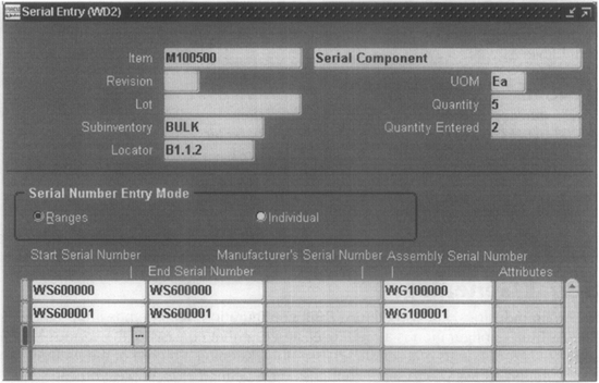
FIGURE 15-5. The Serial Entry form allows you to build the As Built configurations during the WIP Completion transaction

Once you build your serial genealogy, you use the Serial Genealogy form to browse the genealogy of a parent item. You can access this form by clicking the View Genealogy button in the View Serial Numbers form.

On-Hand Balances

The On-Hand balance model keeps track of the inventory that is on-hand and inventory that has been committed to some type of demand, among other things. You can view the on-hand balance information of an item using the View On-Hand Quantities form. Based on the function security of your responsibility, you will be able to view the on-hand balances of your current organization or across organizations. You can choose to view the quantity by revision, subinventory, and locator.

The Quantity Tree

The quantity tree is a memory structure that holds inventory information of each item in memory, in the form of a tree. This information will be stored in nodes at different levels that represent the inventory control levels of an item—revision, lot, subinventory, locator, and LPN. Figure 15-6 shows the node levels in the quantity tree. The tree is kept in synch with the underlying tables when information about an item changes.

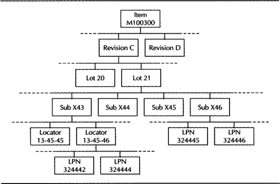
FIGURE 15-6. The inventory control levels that form the nodes of the quantity tree of an item

The inventory information that is captured at each of these nodes includes quantity on-hand, reservable quantity on-hand, quantity reserved, quantity suggested, available to transact, and available to reserve. The value at each node is the sum of the values at all the child nodes.

While developing custom applications/reports, you can use the quantity tree to get accurate information about your on-hand quantities. For example, if you want to find the on-hand quantity for an item, use the public API INV_QUANTITY_TREE_PUB.QUERY_QUANTITIES.

NOTE
The Global Inventory Position Inquiry form allows you to check the inventory position across inventory organizations in a single user interface.

Reservations

When a demand arises, a suitable supply is identified and reserved to the demand so that upstream processes, such as shipping, can fulfill the demand. In simple terms, a reservation is an association between a demand and a supply. The Item Reservation form allows you to define and view reservations in an inventory organization. Many demand types are supported by reservations, although all can be reserved only to on-hand quantity.

NOTE
Starting from Release 11 i, the reservations model in Oracle Applications is architected to support reserving any supply to any demand, although some supply types such as WIP jobs, POs, and In-transit Inventory are not enabled yet.

Implementing Consigned Inventory

Separating the accounting function from subinventory in OWM is the first step taken by Oracle to support consigned inventory. Prior to OWM, a popular workaround for implementing consigned inventory is to use Subinventory as a purely logical entity. For example, assume that you have suppliers S1 and S2 supplying you the item M100500. You may want to stock this item always in a single physical location—01-01-01. In this case, you define two subinventories in the name of the suppliers—S1 and S2 and define two locators in the system—S1-01-01-01 and S2-01-01-01. These two locators in the system point to the same physical location 01-01-01 in the warehouse. Having multiple representations of the same physical locator in the system makes it very difficult to implement various OWM features. For example, you cannot accurately estimate your locator capacity.

With the separation of the accounting function from subinventory, you can implement consigned inventory using cost groups, and at the same time, you have a locator defined only once in the system.

You can use the cost group rules to implement some of the consigned inventory scenarios. For example, you can set up a rule to implement pay on use like this: if a transaction occurs to move material out of this locator, and if the From Cost Group is S1 (for Supplier1’s cost group), the To Cost Group should be POU (for Pay On Use cost group.)

The complete solution on consigned inventory that includes the following features is being developed, but the release schedule was not known at press time.

Ability to establish various event points when the ownership is transferred

Automatically notify payables about the receipt transaction and trigger the payment process

The Rules Framework

OWM comes with a flexible rules framework that is used by various OWM features to identify a target value based on a set of rules. For example, putaway uses the rules engine to identify the most optimal storage location considering factors such as case volume case weight, and locator capacity among others. Almost all the essential data objects in Oracle Applications and their associated attributes are enabled for use in the rule definition, including the descriptive flexfield values for these entities. In this section, the OWM rules engine is discussed in detail followed by the various applications of the rules engine.

Business Objects

Business objects is a common name for all the entities in Oracle Applications that support your business. Examples of business objects are Organization, Item, item Category, Subinventory, and so on. You can use the attributes of these business objects as criteria while defining your rules. For the item business object, examples of attributes include Item Name and the item attribute Inventory Item, among others. You can also use all the enabled descriptive flexfields of the various business objects as attributes in the definition of rules.

The rules framework is seeded with a rich set of business objects. This framework also stores the relationship between the corresponding business object and the context-sensitive operation (that is, Pick, Putaway, Labeling, Cost Group Assignment, and Task Management). Thus, defining new business objects involves defining these complex relationships with the appropriate transaction, which is a technically involved step.

Rules

Rules consist of four key elements: restrictions, sort criteria, quantity function or return value, and (optionally) consistency. Restrictions are constraints that must be satisfied in order that the rule returns a valid dataset. Restrictions are applied on the superset to achieve domain reduction. Sort criteria identifies the order in which you present the reduced domain to the transaction process from a perspective of consumption.

Quantity function determines the formula by which you identify available stock or location capacity. In some rules, quantity function is not used; instead a direct return value can be specified. Consistency allows users to model the resultant set to be consistent within a batch or location. Figure 15-7 shows the OWM Rules form that is used for defining the various types of rules.

FIGURE 15-7. Configure your rules in the OWM Rules form

The rule type identifies the application for this rule. The rule types supported in the current release can be for picking, putaway, cost group assignment, task type assignment, and label selection.

The suggestion are directly specified or derived using a function. Picking and putaway rules use function-based suggestions. The quantity function for picking rules checks for the available quantity, whereas the quantity function for putaway rules checks for available capacity. Cost group assignment, task type assignment, and labeling rules use direct return values. Additionally, task type assignment and labeling rules can be assigned with a rule weight, which will determine the ordering of these rules during evaluation.

Rule assignment can be organization-specific or common to all organizations. Indicate this using the Common To All Orgs check box. For picking rules, you can indicate whether this rule should consider the pick UOM of the subinventory or locator before considering the locator. Pick UOM was covered in detail in Chapter 2.

Each row in the Restrictions tab is a restriction within a rule. A restriction is a logical expression. Consider the comparison A > B. This logical expression has three parts—two operands and a comparison operator. In the restriction, the left operand is a combination of a business object and a object parameter. The right operand could either be a combination of a business object and an object parameter or a constant value, or it could be derived from a value set as well. The value in the operator column links these two sides. Each restriction is identified by the restriction sequence. Grouping restrictions within the rule is achieved by the AND/OR and (“ ”). These columns are useful for modeling complex logical expressions.

NOTE
If you want to use a dynamic list of values on the right side for comparison, choose the right hand object as Expression. For the Expression object, you can include a SQL statement in the parameter field, which should evaluate to your dynamic list of values during runtime.

The Sort Criteria tab allows you to sort the picking or putaway suggestions based on certain criteria. This sortation logic allows you to break the ties between two or more suggestions while generating a suggestion. For example, if your picking sort criteria is to sort the possible results in ascending order of the expiration data (FEFO—First Expire First Out), the lots that expire first are suggested first.

The Consistency tab is applicable only for picking rules, and it allows you to specify certain criteria that must be met by all the picks suggested by the rule. For example, you may want to specify that all the picked items should belong to the same lot. Another example might be to get all the items from the same locator. Thus, consistency can be used to establish certain business rules (picking from a single lot) and also for optimizing your warehouse activities (picking from the same locator.)

OWM is packaged with several seeded rules. To create user-defined flavors of these seeded rules, users can copy these rules and modify the content of the rules in their copy. Rules, once defined, may be edited before being enabled. When you complete your definition, enable the rule by using the Enabled check box. When you enable a rule, the rule verification process checks for the validity of your rule. Typical checks include proper usage of parentheses and appropriate data values (string, number, and so on). You cannot edit an enabled rule. To edit the enabled rule, users need to first disable it. This is done to prevent active rules from being modified.

Strategies

Strategies are collections of rules in a specific sequence. The rules within a strategy are evaluated one after the other until the required suggestions are generated. Figure 15-8 shows the Strategies form, which allows you to define strategies and associate rules with strategies.

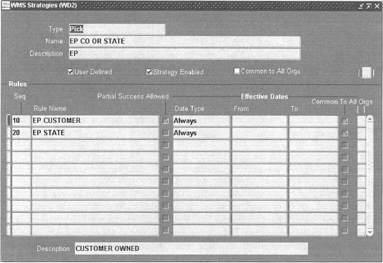
FIGURE 15-8. Create strategies and assign rules in the OWM Strategies form

TIP
Often, the flexibility offered by the rules engine results in different approaches in modeling the same constraint. As a norm, choose the approach that has fewer rules. This may result in improved runtime performance.

When you assign a rule, you specify whether the rule can return with partial success by using the Partial Success Allowed check box. This helps users model the “All or None” scenario.

Each rule that is assigned to the strategy can be assigned with an effectivity. This effectivity control allows you to set up time-dependent and seasonal rule assignments. For example, certain rules may not be applicable in the winter season, whereas certain others may become invalid during the summer season. You specify the effectivity by using the three fields: Date Type, From, and To. Table 15-2 lists the different date types that are available with a short explanation and example From and To values.

TABLE 15-2. Data Type, From, and To Allow You to Set the Effectivity of Rules Within a Strtegy

TIP
Sequence the rules within each strategy considering the priority of evaluation. For example, a customer-specific rule should be evaluated before an item-specific rule and should be listed ahead of the item-specific rule. Always ensure that your last rule is broad enough to generate a suggestion.

Rule assignment can be organization-specific or common to all organizations. Indicate this using the Common To All Orgs check box.

Strategy Assignments

Strategies are assigned to instances of business objects. For example, the strategy HazMatPick can be assigned to the item M100300, which is a hazardous chemical. When you associate a strategy to an instance of a business object, you are essentially establishing a policy at that business object level. Figure 15-9 shows the Strategy Assignments form.

FIGURE 15-9. Assign strategies to business objects in the Strategy Assignments form

You can associate each business object with three strategies—one each for pick, putaway, and cost group assignment. When a picking suggestion is generated for this business object, the assigned pick strategy is used. Similarly the putaway and cost group strategies are used when the appropriate suggestions are generated.

Let’s explain the strategy assignment process with an example. A strategy called STANDARD is considered applicable to all items in an organization and hence is assigned at the organization level. A zone that stores hazardous chemicals in this organization is assigned with a strategy called HAZMATZON. Within that zone are certain locators that store items that need a different way of handling. A strategy called HAZMATLOC is assigned to each of these locators. Finally, certain items require much more specialized handling. Strategies that satisfy those requirements are created and assigned to each of those items. The strategy search order for item, locator, subinventory, and organization is 1, 2, 3, and 4 respectively. In this example, strategies were established at four levels. Figure 15-10 illustrates the applicability of the four levels of strategy assignment.

FIGURE 15-10. Objects that have wider applicability should be assigned with strategies that have a broader perspective and should be accorded lower priority in the strategy search order

When you assign strategies to business objects, assign strategies that are broader in nature to objects that have a wider applicability. Once you establish these broader strategies, you should concentrate on exceptions. Because every activity happens within the context of an organization, consider establishing a very broad policy at the organizational level.

TIP
You can find the rule and strategy that resulted in generating the suggestion in the Material Transaction History.

You can assign strategies to business objects with effectivity. The effectivity options available at the rule assignment level (listed in Table 15-2) are available during strategy assignment as well.

Effectivity control during rule assignment and strategy assignment is offered for greater flexibility. In most cases, it is possible to achieve the same results using effectivity control at one of these levels as illustrated by Figure 15-11. If two or more currently effective strategies are assigned to a business object, the strategy with the lowest sequence number will be used.

FIGURE 15-11. You can establish date effectivity at both the rule assignment level and the strategy assignment level

The level of flexibility is often associated with ease of use. As the level of flexibility increases, the level of complexity increases. In areas where there’s a lot of flexibility, it is better to establish some procedural controls. Because you have to test your rules for various conditions before releasing it for production, consider making a policy in your organization that your effectivity controls are used only at one of these levels. This way, if you get unexpected results, it’s easier for you to troubleshoot at one place rather than going back and forth between two places.

Strategy Search Order

Strategy search order specifies the business object hierarchy within an organization, which is used by the rules engine to select the appropriate strategy. For example, you can associate the picking strategy OrgPickStrategy at the organization level and the strategy HazMatPickStrategy for a set of items. The intent for this is to use HazMatPickStrategy for certain items and OrgPickStrategy for the remaining items. In this case, you should specify the strategy search order as item and then organization.

During strategy search, the business object with the lowest search order is accorded the highest priority.

NOTE
Strategy search order identifies the hierarchy of business object-level policies. Establishing the strategy search order is a one-time step that you perform as part of the implementation process. It is analogous to establish policies ahead of conducting business.

You specify the strategy search order using the Strategy Search Order form. When you establish your strategy search order, give higher priority to the objects that might need special handling. Item-level strategies, for example, would need to be accorded a higher priority than the organizational-level strategy.

Where Used Inquiries

OWM provides the strategy and rules Where Used forms to analyze the impact of modifying a rule or a strategy. The OWM Strategy Where Used form shows the object types and object identifiers to which a particular strategy is associated. The OWM Rules Where Used form shows the strategies in which a particular rule is used. When you want to modify a rule or a strategy that is used in production, use these Where Used forms to analyze the impact.

Rules Logical Data Model

The rules framework consists of four important entities: business object, strategy, rule, and restriction. The logical data model in Figure 15-12 highlights these entities and the relationships between them. It also shows the strategy search order that is established as a part of the initial implementation.

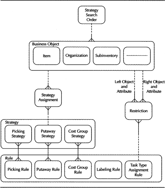
FIGURE 15-12. The rules framework logical data model highlights the important entities in the rules framework

As shown in the figure, although the business objects are common across the framework, rules and strategies are designated for specific business purposes. For example, the Picking Rule and Picking Strategy address the business problem of picking within the rules framework.

Applications of the Rules-Strategy-Business Object Framework

The picking, putaway, and cost group assignment processes use the Rules-Strategy-Business object framework to generate suggestions. The suggestion generation process is shown in Figure 15-13.

FIGURE 15-13. The suggestion generation process for applications in the Rules-Strategy-Business Object framework

NOTE
If after applying a strategy the rules engine is not able to come up with the required results, organization level defaults will be used.

The picking, putaway, and cost group assignment rules use this framework. Note that although you may have a number of strategies assigned to various business objects, only one strategy is used for a suggestion. Once a strategy is selected using the strategy search order, the rules within the strategy are executed to generate the suggestion. If even after applying all the rules, the suggestion cannot be completed, the rules engine does not go back to the strategy search order to pick the next strategy.

Applications of the Standalone Rules Framework

The task type assignment and labeling rules use the Standalone Rules framework. These rules have a rule weight that is used by the rules engine to sequence the rules before evaluating each of them.

TIP
Understanding the Standalone Rules framework is easy if you assume that all the rules you are defining here are assigned to one strategy that is assigned to the business object Organization.

Because these rules have specific return values, there is no question of partial suggestions. So, when the rules engine finds a rule that satisfies all the conditions in the input record, the return value is returned, and the process is terminated.

TIP
You should have a rule in each organization with the least weight that does not have any restrictions, to make sure that every possible scenario is covered. When no other rule results in a suggestion, you can rest assured that the rule with no constraints will result in a suggestion.

Inventory Accuracy

Maintaining the accuracy of inventory is one of the prime objectives of the materials management function. Inaccurate inventory can cause severe losses due to inaccurate order promising, inaccurate production sourcing, and material obsolescence. Physical inventory, which is one of the means of ensuring inventory accuracy, is a legal statute in certain countries. Company auditors are required to check the on-hand inventory before finalizing the balance sheet.

The Oracle E-Business Suite offers two primary methods for verifying inventory accuracy: cycle counting (which relies on ABC analysis and classification of inventory), and physical inventory. These two methods are discussed in the following sections.

ABC Analysis

ABC analysis provides you with the ability to rank your items according to a criterion and prioritize the list of items so that you can establish better material control methods for items with a higher rank. When you perform warehouse control activities such as cycle counting, you make use of one of the pregenerated ABC compilations.

ABC Compiles

You define ABC analysis in the Define ABC Compile form. The Content Scope allows you to decide on the items that you want to include in the analysis—all items in the organization or only the items in the specified subinventory. If you use Organization as the content scope, all the items that are enabled in the organization are included in the analysis; if the content scope is Subinventory, all the items that have a defined item-subinventory relationship with this subinventory are included in the analysis. As far as the content scope is considered, the current on-hand quantity and item cost are irrelevant. That is, items with zero on-hand quantity and zero cost are included in the analysis.

The Valuation Scope is used for ranking the items within the ABC compile. If your content scope is Organization, your valuation scope is automatically Organization. If your content scope is Subinventory, you can set the valuation scope to be either Organization or Subinventory.

If you set the valuation scope as Subinventory, the items that are included in the analysis are ranked based on their position within the subinventory, according to the chosen criterion. For example, assume that you have items M100000 and M100010 in the subinventory with a quantity of 5 and 20 respectively. When your compile criterion is Current on-hand quantity, item M100010 will be ranked higher than M100000.

NOTE
Compiles based on on-hand quantity is shown as a simple example only; most experts would recommend that a compile be generated on a basis that includes both usage (either historical or projected) and unit value. Oracle provides these methodologies as well.

If your valuation scope is Organization, the items that are included in the analysis are ranked based on their position in the whole organization, according to the chosen criterion. Extending the example from the previous paragraph, if the quantities of M100000 and M100010 at the organizational level are 200 and 100, respectively, item M100000 will be ranked higher than M100010.

ABC analysis is a very general term. The Compile Criterion allows you to rank your items based on various criteria. Some of the standard classifications that are used in the industry are discussed in the following paragraphs, along with the respective compile criteria.

FSN Analysis

The classifications fast moving, slow moving, and nonmoving (FSN) are used for ranking items so that you can stock the fast moving items closer to the shipping docks and periodically dispose of the non-moving items. If you create an ABC compilation with one of three material usage quantity criteria—Historical Usage Quantity, Forecasted Usage Quantity, or MRP Demand Usage Quantity—the resulting ABC compilation would be an FSN compilation.

Unit Cost Grouping

Classifying your materials based on their unit costs is currently not supported by any compile criterion. You can achieve the same results by setting up a new subinventory (non-nettable, non-ATP, and nonreservable). Using a custom script, load all the items into this subinventory with a quantity of one. Perform a subinventory level ABC compilation for this subinventory with the current on-hand value as the compile criterion. This will produce a compilation that is based on the unit cost of the item.

Once you finish generating a compilation, have a custom script remove all the items from the subinventory by transacting the material out. If you want to recompile your ABC assignments, you can reload all the items again and then perform the compilation.

Usage Value Analysis

When you want to classify your items based on their overall usage value, you choose one of the usage value criteria: Current on-hand value, Historical usage value, Forecasted usage value, or MRP demand usage value. Usage value analysis gives you the effect of considering both unit price (which is the criterion for unit cost grouping) and usage quantity (which is the criterion for FSN analysis).

Management by Exception

When you want to rank your items based on the problems encountered during the previous cycle count, use either Previous cycle count adjustment quantity or Previous cycle count adjustment value. This way, you can exercise more control over items that have problems during a cycle count.

Sometimes, the number of transactions that happen on an item is an indicator of the potential number of inaccuracies that can result on an item. If you want to rank your items based on the transaction volume, you use Historical number of transactions.

ABC Classes

ABC Classes are used for identifying the item groupings within an ABC classification. You can define the classes to suit the terminology in your company. For example, you can use the standard terms A, B, and C, or you can define High, Medium, and Low for ranking items by usage value. Similarly, fast, slow, and nonmoving would allow you to rank items based on usage quantity. Furthermore, you can have as many classes as you need.

ABC Assignment Groups

ABC assignment group links an ABC compile to the various ABC classes that are assigned to the assignment group. To assign items to the classes, click the Assign Items button. For example, you could assign the classes High, Medium, and Low to the ABC assignment group with the top 5 percent of items in the High class, the next 15 percent in the Medium class, and the last 80 percent in the Low class. To manually include items or update the item assignments, click the Update Items button.

Cycle Counting

Cycle counting is a procedure in which a selected list of items are physically counted to verify the on-hand quantities of those items. Unlike Physical Inventory, which typically counts all the inventory in an organization once a year, cycle counting normally involves continuous counting of a subset of inventory on a regular cycle, usually prioritized by ABC classification. For example, you will count your A items more frequently than your B or C items.

Cycle counting offers a number of advantages when compared to physical inventory:

Fewer items are counted each day, so there is less disruption to normal production or distribution operations.

Although all items are normally counted in the course of a yearly cycle, the high-value (A an B) items are counted more often, providing bigger “bang for the buck.”

More frequent counting of high-value parts offers a much better opportunity to identify and correct the causes of error, rather than just fixing the numbers.

Cycle counting often relies only on the material handling professionals in an organization, and thus can be inherently more accurate. By contrast, physical inventory often requires that all personnel on the shop floor (and sometimes the front office) participate in the count. A wry sage once remarked, “There are three kinds of people in world—those who can count and those who can’t.” In a physical inventory, the mass mobilization of resources often involves the use of people who simply “can’t count.” This is not because of skill or intellect, but just because the office workers may not know proper item identification or the correct unit of measure. Physical inventory sometimes results in creating as many errors as it corrects.

In areas where physical inventory is not a statutory requirement, many companies have been able to satisfy their auditors with a good cycle counting program and thus can avoid the disruption of an annual physical inventory.

You can define and maintain an unlimited number of cycle counts. For example, you can define separate cycle counts for each of your zones.

You define a cycle count in the Cycle Counts form. The cycle count header contains a set of parameters including the cycle count name. The workday calendar is used to determine the days on which cycle count needs to be scheduled automatically. The general ledger account is used to charge cycle count adjustments.

The Control, Scope tab allows you to specify the last effective date after which the cycle count becomes inactive. Enter the number of workdays that can pass after the date the count request was generated before a scheduled count becomes a late count. Enter the sequence number to use as the starting number in the next count request generator. The count sequence number uniquely identifies a particular count and is used in ordering the cycle count listing.

Specify whether you can enter counts for items not scheduled to be counted and whether to display system on-hand quantities during count entry. Specify whether items with out-of-tolerance counts should be automatically assigned with a status of Recount and included in the next cycle count listing. If the cycle count is not for the current organization, you can navigate to the Subinventory region and select the subinventories to include in the cycle count.

The Count option in the Serial Control, Schedule tab is used to specify whether to exclude serialized items from the cycle count, create one count request for each serial number, or create multiple serial details in a count request. The Detail option allows you to specify if you want to capture serial numbers during the count process. If the detail option is Quantity Only, serial number entry is optional if the count quantity matches the system quantity. The Adjustment option allows you to specify if the discrepancies can be automatically adjusted or if every count needs to be reviewed by the approver.

You can enable the cycle count for automatic scheduling. If you turn automatic scheduling on, you should specify the Frequency of scheduling—daily, weekly, or by period. This information is used, along with the count frequency of each cycle count class, during automatic cycle count scheduling. The value you enter here dictates the amount of time that is available to complete the generated cycle count requests. The last scheduled date is displayed for informational purposes. The next scheduled date is also displayed, although you can enter a different date to override the automatically scheduled date.

In the Adjustments, ABC tab specify when approval is required for adjustments. If you choose Never, all adjustments are automatically performed. If you choose Always, all the cycle counts need to be approved before they can be adjusted. Only the counts that are out of tolerance need to be approved if the approval option is Out Of Tolerance. The Hit/Miss% is used for hit/miss reporting. A count is considered a hit if the count variance is within the Hit/Miss% from the system quantity.

The cycle count item initialization or update is based on the Group that is specified in the ABC initialization or update information. If the initialization option is None, the existing list of cycle count items is not changed. The (Re)initialize option deletes existing information and reloads the items from the ABC group. The Update option results in updating any ABC classification changes and allows you to indicate whether to delete unused item assignments that are no longer referenced in the specified ABC group.

Cycle Count Classes

You enter cycle count classes in the Cycle Count Classes window. You can enter ABC classes to include in your cycle count. You can also enter approval and hit/miss tolerances for your cycle count classes. For each class that is included in the cycle count, enter the number of times per year you want to count each item in this class.

You can enter positive and negative tolerances for each class, which will override the tolerances at the cycle count header level. The tolerances are of two types—quantity and value. The Hit/Miss% for the class overrides the Hit/Miss% of the cycle count header.

Including Items in a Cycle Count

You need to load items into your cycle count before you can schedule or count them. You can either enter the items manually in the Cycle Counts window or automatically include items based on an ABC group. You specify an ABC group from which to load your items and all items in the ABC group you choose are automatically included in your cycle count. The ABC classes for that ABC group are also copied into the current cycle count classes and the classifications of the included items are also retained.

Once you have generated your list of items to count from an ABC group, you can periodically refresh the item list with new or reclassified items from a regenerated ABC group. Using the Cycle Counts window, you can choose whether to automatically update class information for existing items in the cycle count based on the new ABC assignments. When you choose the items to include in your cycle count, you can specify which items make up your control group. The control group items can be included in a cycle count every time when you generate automatic schedules, regardless of their schedule frequency.

Cycle Count Scheduling

You can schedule cycle counts either automatically or manually. The number of items in each cycle count class, the count frequency of each class, and the workday calendar of the organization are used to determine the items that need to be included in the scheduled cycle count. In the case of automatic scheduling, the Cycle Count Enabled item attribute should be set to Yes for the items you want to include in the cycle count, and automatic scheduling should be enabled when you define your cycle count.

To generate automatic schedules, invoke the Cycle Count Scheduler from the Tools menu. In the Cycle Count Scheduler Parameters window, indicate whether to include items belonging to the control group. The auto scheduler schedules counts only for the schedule interval you defined for the cycle count header.

You can also manually schedule counts using the Manual Schedule Requests window. You can request counts for specific subinventories, locators, and items. You can manually schedule specific items or all items in a subinventory. If you enter an item and a subinventory, the item is scheduled only in this subinventory.

Count Requests

After you have successfully scheduled your counts, the process Generate Count Requests should be submitted to generate count requests. This process takes the output of the automatic scheduler and the manually scheduled entries and generates a count request with a unique sequence number for each item number, revision, lot number, subinventory, and locator combination for which on-hand quantities exist. These count requests are ordered first by subinventory and locator, then by item, revision and lot.

If OWM is enabled for an organization, these count requests can be dispatched as tasks to the users who are performing the cycle counting one-by-one.

Cycle Count Approvals

The Count Adjustment Approvals Summary window allows you to approve the count adjustments that require approvals. You can access this window by choosing Tools I Approve Counts. You can approve or reject the adjustment, or you might ask for a recount.

Physical Inventory

Physical inventory is the periodic reconciliation of physical inventory with system on-hand quantity. In some countries, performing a physical inventory of the legal entity’s assets at the end of the fiscal year is a legal requirement. Oracle provides a fully automated physical inventory feature that can be used to reconcile system-maintained item on-hand balances with actual counts of inventory. Although physical inventory involves physically counting items, just like cycle counting, there are some major philosophical and technical differences:

Physical inventory takes a snapshot of inventory on-hand quantities at the beginning of the process; all adjustments are made against the snapshot quantity.

Physical inventory generates unique tag numbers for recording counts; missing tags can be identified, and “blank” tags can be generated to record quantities of unexpected material that turns up in the process. (With cycle counting, you’d need to use a miscellaneous transaction to report “found” material.)

Physical counts are reviewed, and either accepted or rejected, as a whole. In contrast, cycle count adjustments are performed as each count is entered, provided the count is within tolerance.

Physical inventory has no predefined tolerances; it is a user’s decision to accept or reject the entire count.

See the Oracle Inventory User’s Guide for details on running a physical inventory.

Inventory Planning

Material Planning (MRP and ASCP) was covered extensively in Part II. This section presents an overview of the inventory planning features that allow you to manage your inventory levels using two planning methods—Min-Max Planning and Re-Order Point Planning. Any planning algorithm is concerned with answering two questions—when to order and how much to order. Figure 15-14 shows how the two inventory planning methods handle these two questions.

FIGURE 15-14. Min-Max Planning and Re-Order Point Planning handle when to order and how much to order

You can use only one of the two planning methods for an item at the organization level. You select the planning method for an item by using the item attribute Inventory Planning Method in the General Planning tab. The choices are Min-Max Planning, Reorder Point Planning, and Not Planned. Depending on the planning method that is enabled for an item, additional attributes have to be set up. Optionally, you can enable an item for Min-Max Planning at the subinventory level.

Establishing sources at the organization level and at the subinventory level were covered in Chapter 2. Using the same methodology, you can establish the sources at the item level using the three item attributes: Source Type, Source Organization, and Source Subinventory. These sourcing attributes are available at the subinventory item level as well. You can establish these sources in the Subinventory Item window. When you perform subinventory level planning, the program attempts to get the sourcing information in the following sequence—Subinventory Item, Item, Subinventory, and Organization. When you perform organization-level planning, the sequence is as follows: Item and Organization.

Min-Max Planning

Min-Max Planning allows you to specify the maximum and minimum inventory levels for your items and maintain on-hand balances between these two levels. Min-Max planning triggers a supply order when the quantity on-hand falls below the minimum inventory level. By default, Min-Max tries to restore the inventory balance to the maximum level. For example, if the minimum quantity is 25 and the maximum quantity is 100, Min-Max will create a supply request when the on-hand balance drops to 24. The requisition quantity will be 76. Although Min-Max takes the pending demand and supply into consideration, it does not take the lead time to source or fulfill those quantities into consideration.

TIP
Your minimum inventory level should be set considering the lead-time demand and safety stock requirements. You should also ensure that your Min-Max levels avoid too many orders being placed.

Min-Max does take the order modifiers into consideration while creating the supply request. Order modifiers were discussed in Chapter 8.

Min-Max Planning at the Organization Level

To enable an item for Min-Max planning at the organization level, choose Min-Max Planning as the value for the item attribute Inventory Planning Method. Specify the minimum and maximum inventory levels by using the item attributes Min-Max Minimum Quantity and Min-Max Maximum Quantity, respectively. Depending on the value of the Make Or Buy item attribute, the program will generate either work orders or requisitions as supply.

Min-Max Planning at the Subinventory Level

In the Subinventory Items window, specify the planning method as Min-Max Planning. Specify the minimum and maximum inventory levels using the attributes Min-Max Minimum Quantity and Min-Max Maximum Quantity, respectively. Subinventory-level planning generates only requisitions.

Min-Max Planning Concurrent Program

To perform Min-Max planning, run the Min-Max Planning report. Choose the planning level as Organization or Subinventory. If the planning level is Subinventory, you should select a subinventory. The parameter Restock allows you to specify whether you want to create supply orders. You can set Restock to No to print a report. If you set Restock to Yes, the program will create requisitions or work orders appropriately.

Reorder Point Planning

An item is enabled for Reorder Point (ROP) Planning by using the item attribute Inventory Planning Method. Once you enable an item for ROP Planning, provide the values for all the related attributes—Pre-Processing Lead Time, Processing Lead Time, Post-Processing Lead Time, Order Cost, and Carrying Cost Percentage.

Safety Stock

Safety stock provides the cushion that protects your consuming lines from fluctuations in the supply process. The safety stock level for each item can either be calculated automatically or be entered manually. You can also use MRP or ASCP to dynamically calculate safety stock, as was discussed in Chapter 8.

If you set the attribute Safety Stock Method to Non MRP Planned, you can calculate the safety stock using the methods that are available in the Enter Safety Stocks window. You can use the mean absolute deviation or a user-defined percentage of forecasted demand. Once you’re in this window, select Tools I Reload to invoke the Reload parameters. The choice of methods are Mean Absolute Deviation and User-Defined Percentage.

If you select User-Defined Percentage, the safety stock is calculated as the gross demand for the forecast period multiplied by the value of the parameter Safety Stock Percent. If you select Mean Absolute Deviation, specify the service level. The safety stock is calculated using the following formula:

Safety Stock = Z×1.25×MRD

MAD is the average of the absolute deviations of the historic forecasts from the actual demand. Z is the probability value from the normal distribution that corresponds to the specified service level.

ROP Planning Calculations

When you run ROP Planning, the reorder point is calculated using the following formula:

Reorder Point = Safety Stock + Forecast Demand during Lead Time

The lead time is the sum of the Pre-Processing, Processing, and Post-Processing lead times. Because safety stock is controlled by date effectivity, it is possible to have different safety stock levels during the lead time. In such cases, the largest of safety stock during the lead time will be used. The demand from forecasts during the lead time is added to the safety stock to get the reorder point.

NOTE
ROP Planning uses forecasts as its source of anticipated demand. Because you can only establish forecasts at the organization level, ROP Planning is available only at the organization level.

The ROP Planning process creates a supply request for a quantity that is equal to the economic order quantity (EOQ), when the on-hand quantity is less than the reorder point. The EOQ is given by the formula that is shown here:

The annual demand is calculated by annualizing the current demand rate. The ordering cost and inventory carrying cost are obtained from the item attributes.

ROP Planning Concurrent Program

To perform ROP planning, you run the Reorder Point Planning report. The planning level is always Organization. The parameter Create Requisitions allows you to specify whether you want to create requisitions or not. You can set this parameter to No for simulation runs. If you set this to Yes, the program will create requisitions.

Replenishment Counting

In subinventories where you are not maintaining perpetual on-hand balances, you can use the replenishment counting system to plan your inventories. This may be ideal for replenishing free stock items that you don’t intend to keep track of. You can only use the replenishment counting system at the subinventory level. To use replenishment counting, you must set up item-subinventory relationships using the Item Subinventories or Subinventory Items windows.

You create a replenishment count in the Replenishment Count Headers window. While generating the replenishment, you can choose to specify the order quantity or choose the maximum order quantity from the Min-Max planning settings. You enter the count details through the Replenishment Counts window. The Process Replenishment Counts program processes the replenishment counts and creates requisitions for items that need to be ordered, or it creates move orders for items to be replenished from a subinventory.

Replenishment Tasks

A move order line is created for each item found to need replenishment where the supply source type is subinventory. The move order line is allocated based on the picking and put away rules. (Move order is covered in the section “Move Orders” and rules are covered in the section “The Rules Framework.”) After the lines are allocated, the rules engine is invoked to assign a task type for each task. These tasks are then dispatched to qualified users. (Task type assignment and task dispatching are covered in the section “Task Management.”)

Data Field Identifiers in Barcode Scanning

Barcoding speeds up data entry and avoids data entry errors. All the mobile transaction forms (also called pages) support barcoded data. Data field identifiers (DFI) are used for identifying the type of data that is embedded within a barcode while scanning them using a barcode reader. For example, the DFI for an item number is l+. DFIs allow you to scan data in an arbitrary sequence. That is, if your data entry page has item number followed by the transaction type, you are not constrained to scan these data in that sequence. If you use DFIs to identify these fields, the correct field will be populated regardless of the sequence of scanning. If you don’t use DFIs, the current field will be populated with the scanned information.

NOTE
Oracle Applications comes seeded with industry standard DFIs.

Attribute-Level DFI

The AK Dictionary stores the DFI information. You can also configure your field labels in the dictionary. The Define Attributes form (available from the standard AK Developer responsibility) is used for defining DFIs at the attribute level. The DFI for each attributes is entered in the Default Varchar2 Value field.

Region-Level DFI

Instead of defining DFIs attribute-by-attribute, you can define DFIs at the region level. In the Define Regions form (available from the standard AK Developer responsibility), find the resource table for your application by using the Region ID. For inventory and OWM, the region ID is INVRESOURCETABLE. Once you find the resource table, click the Region Items button. On the Region Items window, locate your appropriate field(s) and specify the DFIs in the Default Varchar2 Value field.

The DFI String

The DFI string always takes the following format:

DFI=Q+, q+, Q, q REQ=N

This DFI indicates that four DFIs (Q+, q+, Q and q) may be used for this field. It also indicates that this field can take values without a DFI. To make the DFI required for a field, use the REQ=Y instead of REQ=N after the DFI list.

CAUTION
DFIs should be listed in the order they should be validated against. In your DFI sequence for a field, if you enter A before A+, this will result in data validation errors for data that have A+ as the DFI. For example, assume that the field is A+M493874. When the mobile server reads this value, it immediately resolves it based on the first character and identifies the field because there is a match for A before A+. So the field value would be +M493874. To avoid this, arrange your DFI list from most specific to least specific. In this example, A+ should come before A in the sequence.

Compliance Labeling

Customers might require you to ship your items with a label that suits them. Sometimes, you may be required to provide different kind of information in your labels to comply with the legal requirements of the state or countries in which the transaction takes place. The compliance labeling support provided by OWM allows you to handle these and similar requirements.

NOTE
The tables WMS_LABELS and WMS_LABEL_FIELDS store the information about labels.

Label Types

Label types identify what information is applicable to a particular label format. Oracle has provided eight label types: Material label, Serial label, LPN label, LPN Contents label, LPN Summary label, Location label, Shipping label, and Shipping Contents label. These label types are associated with a set of fields. When you define a label format, the list of fields is restricted based on the label type that you choose.

Business Flows

Within OWM, business flows represent the various transaction points where a label may be required. For example, Receipt is the business flow that represents receiving materials. OWM has enabled 22 business flows for which you can automate label printing.

Assigning Label Types to Business Flows

Once all the label types and the business flows are defined, assign the appropriate label types to each business flow. The Assign Label Types to Business Flows form that is shown in Figure 15-15 allows you to do that. As a part of executing each business flow, Oracle will generate an XML file and write this to a specific directory. The labeling software (third-party software) has polling processes that take each XML file, generate the label, and direct it to the appropriate printer.

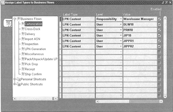
FIGURE 15-15. Assign label types to business flows to indicate label usage

NOTE
Not all the label types can be associated with every business flow. For example, Location label types cannot be associated with the Receipt business flow. Please refer the product documentation for OWM to check if a particular label type can be associated with a business flow.

Label Formats

You define label formats by using the Define Label Formats form. Each label format is based on a label type. You can disable a label format by using the effectivity date. The Default Label check box allows you to specify the default label for a particular label type. If the rules engine is not able to suggest a label format based on the available rules, the default label format for that type will be suggested. You can have only one label format as the default for each label type.

NOTE
Label format rules were covered earlier in the section “The Rules Framework.” If you want a label format to be considered, you have to define at least one rule with that label format as the return value.

Once you define the label format, you can select all the fields that are applicable in that label format. The Label Fields button in the Define Label Formats form takes you to the Define Label Field Variables window, which allows you to select the appropriate fields for a format. For each field that is selected in a particular format, specify the Field Variable Name that is used for passing information on to the labeling software.

CAUTION
The XML file that is generated contains the name of the label format and the Field Variable Names as tags that identify each field. You should make sure that the labeling software understands these variable names.

Not all printers are capable of printing all the labels. So, once you have defined your label formats, associate each label format with the appropriate printers by using the Choose Document and Label Printers form.

The Label Generation Process

When a business flow is being executed, one label format per applicable label type will be returned based on the label format rules. For each label format, an XML file is generated, based on the label format definition. This XML file will be read by a labeling software, which interprets this information and prints the appropriate label.

Container Management

The Container Management feature in Oracle Applications allows users to define containers in and pack/unpack materials into these containers. Users have visibility to the contents of containers and can transact material by container instead of individually.

Containers are items. A container item is identified using the Container flag in the Physical Attributes tab of item attributes. The Physical Attributes tab that is shown in Figure 15-16 also contains other physical attributes, such as the container type, internal volume, maximum load weight, and the minimum fill percent of the container item. These capacities will not prevent the user from overpacking but will issue a warning if a user attempts to put more items in a full container.

FIGURE 15-16. Define the physical attributes of container items in the Items form

The attributes in the sections Weight, Volume, and Dimensions apply to both container and contained items. This information is used as packaging constraints by the cartonization process while generating packaging recommendations.

CAUTION
Weight, Volume, and Dimensions should all be entered for each of the container and contained items. If any of this information is not defined, cartonization will fail. Cartonization is covered later in this chapter.

Because containers are items, they can be replenished through inventory replenishment mechanisms such as the Min-Max or ROP planning. Containers can be planned as other items if they are included on the bill of materials for the finished goods they are used to store. This enables users to forecast their container requirements. As with other items, a user can view the on-hand balances of containers in a particular inventory location.

Typically reusable container items are serial controlled. The serial number serves to identify the container instance during its life. Reusable containers will be supported in a future release of OWM.

License Plate Numbers

A License Plate Number (LPN) serves as a unique identifier for each individual container. LPNs can be pregenerated and associated with containers at a later time. So, an LPN need not be associated with a container item when the LPN is created. The pregenerated LPNs that are not associated with any container item do not have any container item’s characteristics, such as capacity, dimensions, and so on.

You specify the default prefix, default suffix, and the starting LPN Number Revision, Lot, Serial, LPN tab of the organization parameters by using the Prefix, Suffix, and the Starting LPN Number fields in the LPN Generating options. You generate LPNs by using the Generate LPN concurrent program.

LPN is not the same as the container item serial number. The serial number of a container item is used to track the container during its entire life, whereas during the course of its life the container may be associated with many LPNs depending on the number of times the container was cycled through different warehouses and manufacturing plants.

NOTE
The tables WMS_LICENSE_PLATE_NUMBERS, WMS_LPN_CONTENTS, and WMS_LPN_ HISTORIES store all the LPN information.

At the LPN (container instance) level, OWM stores information about the contents and location, status, a history of all transactions, and whether the container has been sealed. Sealed containers cannot be packed, unpacked, or partially reserved. You can view the on-hand balances of LPNs of a particular container item as well as the balance of the unused container items that do not have an associated LPN.

The transaction history and current location of each LPN is stored by OWM at all times. They could reside in the following:

Receiving

Inventory (in a subinventory and locator)

WIP (used for packing, as assemblies are completed)

Transit (notice sent through an advanced shipment notice [ASN] or interorg transfers)

Trading partner site

The LPN Contents form allows you to view the contents of a specific LPN. The top-right block provides information on the LPN itself, including location, associated container item, and LPN number. The left panel provides a tree view of the hierarchy of containers. In the lower-right block, the contents of the highlighted LPN on the left pane is displayed. Contents can be items or containers. If the item is lot- or serial-controlled, you can view that information using the Lot/Serial button. Figure 15-17 illustrates how you can use the mobile forms to view the contents and details of an LPN. You can also use the Material Workbench to view the contents of an LPN.

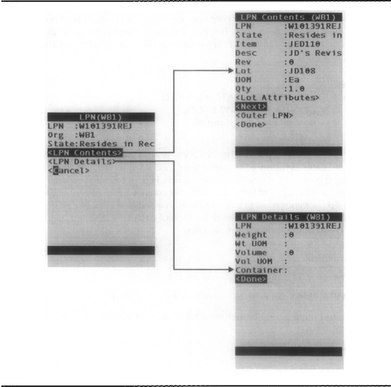
FIGURE 15-17. You can view the contents and details of an LPN by using mobile LPN inquiry

Cartonization

Cartonization simplifies the process of deciding which container to use for a particular packaging problem. The cartonization process automatically suggests packing configurations for groups of items considering various packing constraints. The category Set Functionality that was discussed in Chapter 3 is used for grouping container items and content items.

Cartonization Group Definition Using Category Sets

Container items and content items are classified into cartonization groups by using the two seeded category sets—container items and content items. Before defining categories and assigning them to these seeded category sets, decide on the control level of these category sets. If you want to follow a uniform cartonization scheme (centralized scheme) across all organizations, choose the control level as Master. If you want each organization to design their cartonization scheme (decentralized scheme), choose the control level as Organization. Figure 15-18 illustrates the concepts of container items and content items.

FIGURE 15-18. Container items and content items are linked using a cartonization group

The container items and content items are matched using these seeded category sets. For this reason, both these category sets must have the same category codes. For example, you can have a category called HAZARDOUS in both of these sets. Assume that HCASE1 and HCASE2 are used for packing hazardous materials. HCASE1 and HCASE2 will be assigned to the HAZARDOUS category under the container items category set. If you have two items called Phenyl Alcohol and Sulphuric Acid, and if you want them to be packed using the hazardous packing material, these items will be assigned to the HAZARDOUS category under the Content Items category set. If the cartonization process has to find a suitable container for the item Phenyl Alcohol, it will look at all the suitable containers that belong to the category HAZARDOUS in the Container Items category set.

NOTE
The cartonization group is defined by the category code. All the container items that belong to a category code within the Container Items category set and all the content items that belong to the same category code within the Content Items category set form a single cartonization group.

Container Item Relationship

The cartonization group establishes generic relationships between cartonizable items and containers, treating them as whole groups. This may not be enough for handling certain items, which must be placed in certain kinds of containers. These items could have container load relationships specified using the Container Item Relationship form. This is a direct relationship between a content item and the container item.

To include a container in the container item relationships, check the Container flag in the Physical Attributes tab of the item. Because the quantity is defined in this relationship, the physical attributes of the content item or container item are not considered during the cartonization process.

Cartonization Process During Sales Order Release

The pick release process groups the pick-released lines based on delivery grouping rules. Each pick-released line will belong to one delivery group. (Deliveries are covered in detail in Chapter 16). A subset of the lines within each delivery group could be cartonizable, depending on whether the Enable Cartonization flag is turned on either at the organization level or the subinventory level.

Within the cartonizable lines, all the items that have a container item relationship defined are selected and cartonized. For example, a line has a quantity of 1000 for the item M100200. A container item relationship exists for this item that says that this item can be packed in a container called C300, and the quantity of M100200 per container is 120. The cartonization process will suggest nine containers—eight containers with 120 each and one container for the remaining 40. This will result in nine pick tasks from one picking line. Nine LPNs will be generated automatically as the suggested LPNs. You can ignore the suggested LPN and use your own if you want. Tasks are covered later in this chapter.

NOTE
The cartonization process assumes infinite availability of container items.

All the remaining lines that have items without a Container Item Relationship are assembled into subgroups that have the same Cartonization group.

The cartonization process tries to fit the entire subgroup in one container, if possible. The containers in the group are ordered from the smallest before starting the comparison. The comparison starts from the smallest container to check if it fits the entire subgroup of items. If not, the next bigger container is checked until a container that fits all the items is found or the largest container is reached.

NOTE
Container volume is used for ordering the containers from largest to smallest. While actually assigning items to the container, capacity in terms of both volume and weight are checked.

When the largest container is not sufficient to hold every item in the subgroup, the cartonization process assigns the portion of items that will fit in the largest container. Before assigning each item, the dimensions of each of the items are compared with the dimensions of the container.

NOTE
During dimension comparison, the largest dimension (among length, width, and height) of a content item is compared with the largest dimension of the container item; the second largest with the second largest; and the third largest with the third largest.

The remaining items are cartonized using the same process, starting from the smallest container in the group.

NOTE
Cartonization using a container item relationship does not suggest mixing different items in the same container. Cartonization using Cartonization groups suggests mixing different items in the same container.

Container Transactions

Container transactions allow you to transact material in bulk without having to worry about the contents. You can create prepack requests for the cartonization process to suggest the appropriate container for your WIP job completions. Once you pack a container with your items, the LPN of the container can be used to move the materials around the warehouse. When you want to take materials out of a container, you can perform an unpack transaction to transfer material out.

Container Prepack

Container prepack is used to suggest appropriate cartons and LPN labels in advance of a WIP completion. You can prepack LPNs in anticipation of the WIP job or schedule completion. A request can be made to pack the finished goods into a container in order to generate labels for the container. During the container prepack transaction, the cartonization process will be used to estimate the container requirements for the items that are to be completed from the Job/Schedule.

The prepacked LPNs will not be included in on-hand inventory. Labels can be printed with content data. The completion transaction will then be performed automatically when the LPN is packed.

Bulk Pack

The mobile Bulk Pack form is used to suggest containers to pack a single item in a particular locator in the warehouse. This might be used if you find a large amount of loose material of an item that should be packed. By leaving the container field blank on the mobile form, the cartonization algorithm is called on the quantity of the item to pack.

Packing Consolidation and Splitting

The mobile forms Consolidate and Split allow you to consolidate multiple LPNs into a parent LPN or do the reverse respectively. Figure 15-19 shows these forms. When you consolidate, you specify a parent LPN and specify all the LPNs that need to be consolidated one by one, by clicking the More button. The Merge button will complete the consolidate transaction. When you split an LPN, you specify the source and destination LPNs and the item and quantity that you’re moving to the destination LPN. The More button allows you to continue with the split transaction. Clicking the Split button will complete the transaction.

FIGURE 15-19. The mobile Uls for packing consolidation and splitting a container

Unpack Transaction

The unpack transaction results in putting the contents of an LPN into a locator as loose quantity or transferring it into another container (LPN). The Unpack mobile form allows you to perform this transaction.

Manufacturing Issue Transactions

Material is issued to Oracle WIP from only loose items and not from an LPN. All the LPNs that contain components that are used in manufacturing will have to be unpacked prior to the issue transaction—both backflush and push transactions.

It may be a labor-intensive task to unpack all the LPNs manually before issuing them to manufacturing. The flag LPN Tracked on the subinventory indicates if the subinventory keeps track of LPNs or ignores the LPN information and retains only the content information. Thus, if the subinventory is not LPN-tracked, all LPNs transacted into that subinventory will be automatically unpacked. Consider turning off the LPN Tracked flag for subinventories that are often used for manufacturing issue and backflush transactions.

Task Management

Task Management is the process of creating, dispatching, and tracking tasks with in a warehouse. The objective is to maximize labor productivity and equipment utilization. Tasks are created by various processes. For example, the pick release process creates picking tasks, and the cycle count request generator creates cycle count tasks. Figure 15-20 shows the important entities that support Task Management.

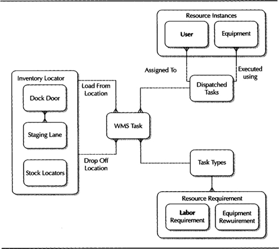
FIGURE 15-20. The important entities in OWM Task Management

NOTE
Tasks are stored in MTL_MATER1AL_ TRANSACTIONS_TEMP. You can identify the task type for each from the WMS_TASK_TYPE column.

As shown in Figure 15-20, each task is associated with one or two locations depending on the type of the task. Picking tasks, for example have a load (pick from) location, and a drop off location. Cycle count tasks, on the other hand, have only one location—the count location. The type of tasks also identifies the resource requirements for each task. Based on the resource requirements and location considerations, tasks are dispatched to users who are qualified and have the appropriate equipment to perform the task. Task Type definition was covered in Chapter 4. OWM task management is built on top of two powerful processes: the Task Type Assignment Engine and the Task Dispatching Engine.

Task Type Assignment Engine

The task type assignment engine is called during the pick release process. Once the rules engine decides on the subinventory, locator, lot, and so on, the task type assignment engine is called and based on the task type rules, a task type is selected and stamped on the allocated line. Task type assignment rules were covered in the section “The Rules Framework.” This engine also performs task splitting and merging based on certain conditions.

Task Type Assignment

Prior to assigning a task type, the resource requirements of a task are not known. For example, you may want to perform task type assignment based on the pick UOM. If the pick UOM is PA (pallet), you may want to use the task type Pallet Picking, which requires a pallet picker and a forklift. Similarly, if the pick UOM is EA (each), you may want to assign Each Picking, which might have different resource requirements. Once the task type is assigned, the upstream processes know the resource requirements for that task.

Task Splitting

After the task type is assigned, the system knows all the possible equipment that can be used to perform the task. Equipment setup was covered in Chapter 4. If the task quantity exceeds the capacity of the smallest equipment available to perform the task, the task splitting engine will split the task into manageable units that can be handled by any equipment within the resource group. Each of those units will still have the same pick slip number and therefore cannot be dispatched to different users. The same user who picks the first unit will have to finish all the split tasks belonging to the same pick slip number.

Task Merging

If any of your items use the pick methodology Bulk Pick or if the lines were released with the pick slip grouping rule set to Bulk Pick, tasks for those items that belong to the same delivery, with the same picking and destination locators, are merged to form a single task for dispatching purposes.

Task Dispatching Engine

The task dispatching engine sequences and dispatches tasks. Tasks are sequenced based on task priority and then on the locator picking order/XYZ coordinates of each locator and the last pick location of the user. These were covered in detail in Chapter 2. The objective of task sequencing is to minimize the distance traveled by each user.

The sequenced tasks are dispatched to users when they press the Accept Next Task button in the mobile Tasks menu. The task is dispatched based on the user’s role, the equipment currently used by the user, and the zone in which the user signed on. The task dispatching process tries to minimize dead heading, that is, users traveling with empty load.

Warehouse Control Board

The Warehouse Control Board is a managerial tool for warehouse managers. It provides a single window from which you can manage the tasks in your warehouse and also to gauge the performance of the warehouse. Figure 15-21 shows the Performance tab of the control board. It shows two pie charts—the first chart shows that all the tasks are completed and the second shows that out of all the tasks that were completed, 21 percent were picking tasks and the remaining 79 percent were putaway tasks.

FIGURE 15-21. The Warehouse Control Board provides you a single Ul from where you can manage your warehouse tasks and analyze warehouse performance

The Task Details tab shows the task, task type, and the role required to perform this task, among many other details. This tab also shows the employees who are performing each task. You can assign/reassign tasks to users in this tab. For example, if the shift ends for a user in the middle of performing some tasks, you can reassign all the tasks that were pending in that user’s queue to another user.

All the tasks that had one or more problems during execution are shown in the Exceptions tab. For example, if a picker is asked to pick 10 items from a location and picks only 9 due to non-availability of material, an exception is recorded in the system. Similarly, if a user who is directed to put away the material in a particular location couldn’t complete the task due to non-availability of space, an exception is recorded in the system.

Receiving and Putaway

Oracle supports receipts, inspection, and putaway for material from any source—suppliers, other organizations, and customer returns. You can easily configure if the material that is received needs to undergo quality tests before it hits your inventory balances through the receipt routings. The rules engine that was covered in the section “The Rules Framework” is used to determine the cost group for the received material and the optimal inventory storage location for a putaway. Receiving was covered in detail in Chapter 14 as provided in Oracle Inventory and Purchasing; it is mentioned here from the perspective of Oracle Warehouse Management.

Creating Receipts

When material reaches the receiving dock, the material is unloaded onto the receiving staging lanes and the receipt check-in is done against the document number that the material belongs to. This document number can be the purchase order number, internal requisition number, inter-org shipment number, RMA number, or an ASN. Along with the document information, you have to scan the information of the material that you’re receiving. Figure 15-22 shows the mobile page flow for the receiving process.

FIGURE 15-22. Receipts using standard receipt routing can be received onto an LPN directly

NOTE
CTRL+G generates LPN, lot, and serial from the mobile device.

Because putaways are always LPN-based, the material that is received should be associated to an LPN. You can use a pregenerated LPN, generate an LPN while performing the receipt, or receive material into an existing LPN. Material could be received into the LPN, and then put away from the LPN into your storage areas.

If you don’t want to use LPNs at all, you can model a transport cart as an LPN. If all subinventories were marked as non-LPN Controlled, OWM will force material to be put away loose, and the cart can be reused for putaways. Similarly, you could model an area on the receiving dock as an LPN and receive into that LPN. When you want to put away, you can specify the LPN that corresponds to the receiving area to take the material from there.

Putaway

When an LPN is scanned for putaway, the rules engine will be used to suggest an optimal putaway location for that material. During the process of the putaway, the user will be asked to confirm certain information about the material being put away, as shown in Figure 15-23. You can choose to accept the default LPN to drop off, generate a new LPN, enter an existing LPN, or leave the field blank. If an entire LPN is suggested to be put away in the same place, the To LPN field will be defaulted to the original LPN. You can leave the To LPN field blank for loose putaway.

FIGURE 15-23. Once you receive goods into an LPN, you can generate putaway tasks to put away the LPN using system-generated suggestions

NOTE
If the subinventory that the material is being putaway to is not LPN Controlled, the To LPN field will be hidden.

NOTE
If the receipt routing requires inspection, the LPN has to be inspected before putaway.

Once you choose an LPN, you can choose to drop it off immediately. Depending on the space in your vehicle, you can decide to load more LPNs by pressing the Load button. Once you’ve completed loading, you can go to the Current Tasks page (covered in the section “Currently Loaded Tasks”) and drop off the LPNs one-by-one.

Implementing Opportunistic Cross-Docking

Cross-docking enables moving material directly from one process to the other without the need for stocking it. This can result in enormous savings in shipping and can also result in improved customer service. Cross-docking can be classified as two types: Opportunistic and Planned. Opportunistic cross-docking is available in the current release of OWM through the shortage handling functionality.

Cross-Docking from Receiving/WIP Completion to Shipping

If backorders exist for an item, Oracle will suggest that the material be put away directly to the outbound staging area for immediate shipment, if cross-docking is enabled for your organization. This happens when you receive items from your suppliers or when you perform assembly completions in Oracle WIP. This opportunistic cross-docking functionality is not available when you perform a direct receipt. Material that has been rejected at time of inspection will not be cross-docked but it can still be put away.

Cross-Docking from Receiving/WIP Completion to WIP Requirements

When shortages exist in WIP jobs, OWM directs the required material to the job/schedule, when you receive items from your suppliers or when you perform assembly completions in Oracle WIP.

If you check the warehouse parameter Prioritize WIP Jobs flag, WIP shortages are accorded a higher priority than sales order shortages. If this flag is not checked, sales order shortages are accorded higher priority. As long as material is available, OWM will try to meet all the shortages.

The Order Fulfillment Process

Order fulfillment is a very important function to the survival of any business. This function can make a huge difference in customer service. Activities in this process include scheduling your docks so that no conflicts arise in vehicle arrival/departure, pick planning, pick execution, staging and consolidation, loading the goods onto the vehicle, and finally, ship confirming. This section discusses these activities in detail.

Dock Scheduling

During trip planning, you can assign each trip to a dock door from which the truck will be loaded. You can create a dock appointment for this trip. You can schedule inbound unload activities or other activities to a particular dock door as well. If a trip has been assigned to a dock door and an appointment has been created for this trip, the pick release process will find the nearest staging lane that is either empty or is likely to become empty soon and direct all the picks for that trip to this staging lane. The staging lane to dock door assignments are performed at the time of setting up the warehouse. Figure 15-24 shows the Calendar form that allows you to schedule your docks for receiving and shipping.

FIGURE 15-24. The Dock Calendar form provides daily, weekly, and monthly views of your dock schedule

Pick Methodologies

In some cases, it is optimal for a warehouse picker to perform multiple picks in each of his pick cycles. When he performs multiple picks, depending on the warehouse configuration and business conditions, in some cases picking the whole order in one cycle might be sensible; in other cases, splitting the order with respect to the zones from where the order has to be picked might make more sense. Pick methodology identifies how a sales order or a group of orders are handled in the warehouse.

NOTE
Internally, each pick task that is generated is stamped with a group ID that is generated based on the pick methodology. The PICK_SLIP_NUMBER column in MTL_MATERIAL_TRANSACTIONS_TEMP is used for storing the group id of each task.

Defining Pick Methodologies

The Pick Slip Grouping Rules form is used to define pick methodologies. The form supports defining four standard pick methodologies and a variety of user-defined pick methodologies. The field Pick Methodology is a drop-down list contains the four standard pick methodologies. Specify the rule name and (optionally) rule description and effective dates. The form also has a Group By section with 12 check boxes. For standard pick methodologies, the check boxes in the Group By region cannot be edited. Figure 15-25 shows the Pick Slip Grouping Rule form.

FIGURE 15-25. The Pick Slip Grouping Rules form allows you to define the various standard and user-defined pick methodologies

Order Picking

When this pick methodology is selected, the Order Number check box is automatically checked in the Group By region. Order picking involves picking one order by a picker, regardless of the number of zones the order needs to be picked from. All the tasks from a sales order are assigned to a single picker. The first eligible picker who accepts the next task gets all the tasks belonging to that order. This is typically used for managing emergency orders or orders from very important customers.

Zone Picking

Both the Order Number and Subinventory check box are automatically enabled in the Group By region for Zone Picking. Zone picking results in the splitting of the sales order by the zones from where the ordered items need to be picked. The pick tasks in each zone-order combination are dispatched to a picker who is assigned to the zone. The picker in this case will specify a subinventory during sign on.

Bulk Picking

An item may appear in a group of orders and instead of picking the item individually for each of the orders, it may make more sense to pick the item as a full pallet or a case and then split it (called the sortation process) across the orders, during the drop process or at the time of staging the material. This pick methodology is called bulk picking. This type of pick methodology is most suitable for high-volume items that need to be picked frequently. When this pick methodology is selected in the Pick Slip Grouping Rules Form, the Item, Locator, Lot, and Revision check boxes are automatically enabled. During the bulk pick process, the tasks are grouped if and only if they belong to the same delivery.

Bulk picks require an additional step—sortation. The picker brings the pallet or case and delivers the quantity required by each delivery in the appropriate staging lanes. At each staging lane, the appropriate quantity will be dropped off onto existing LPNs or new LPNs. Consider an example where a picker is asked to pick a pallet containing 12 cases of an item. Four orders needed this item in the quantity of 2 cases, 3 cases, 3 cases, and 4 cases each. If you used bulk picking, a pallet is picked, and the picker will deliver the required quantity in the four staging lanes that are handling the deliveries of these orders. The sortation and consolidation steps need to be performed manually, using the consolidation report that assists users to consolidate and sort the orders prior to loading them onto trucks.

Cluster Picking

When this pick methodology is selected, none of the boxes are checked. The pick tasks are not grouped by any criteria. The tasks will be sequenced according to the locator picking order and dispatched to the pickers. Each pick task has a unique pick slip number in this case.

Assigning Pick Methodologies to Zones, Items, and Pick Waves

Because order picking and zone picking involve grouping by order, and cluster picking doesn’t have any grouping, the only pick methodology that can be enabled at the item level is bulk picking. You can enable bulk picking for an item by checking the Bulk Picked attribute in the Inventory tab. You should scroll to the right to see the Bulk Picked attribute.

Depending on how you stock material in your zones, you may want to follow a different pick methodology in each of your zones. For example, in zones where you stock your pallets, you might want to follow bulk picking; in zones where you store individual pieces, you might want to follow cluster picking. From Release 11 i.H, you can assign the bulk pick methodology at the zone level. If bulk picking is not turned on, cluster picking is assumed at the zone level. The zone level pick methodology, if assigned, overrides the item-level picking methodology.

A pick methodology can be assigned to a pick wave during pick release. Pick waves are covered in the next section “Wave Picking.” If a pick methodology is assigned to a pick wave, this pick methodology will override the pick methodologies at the item and zone levels.

Wave Picking

Wave picking is the pull-based picking process. Sometimes, waves are associated with vehicle departures. For example, if three vehicles leave your warehouse every hour, one pick wave is released for each hour to fill the three vehicles that leave in that hour. The pick release process allows you to model different kinds of waves. You can create a wave that is based on a trip, delivery, carrier, customer, and so on. When you release your wave, you can select an appropriate pick methodology, if you want to override the methodologies assigned at the item level and zone level. Figure 15-26 shows the Inventory tab of the Pick Release form.

FIGURE 15-26. The inventory options during pick release

If you want to automatically source the material and create reservations, specify Auto Allocate as Yes. You can specify the subinventory and locator to pick from if you want to force a location. If you want to ignore the picking execution process and want to automatically confirm the picks of all the items that are detailed, specify the Auto Confirm option as Yes during pick release.

The pick release process creates a move order of the type Pick Wave. The move order is automatically detailed if the Auto Allocate option is set to Yes.

Staging Lane Assignment for Pick Tasks

Each line that is released for picking will have a staging lane as the destination for the pick tasks. The destination staging lane for each wave can be specified in the Pick Release window by using the Default Stage Subinventory and Default Stage Locator fields.

If a trip is associated with a dock door, the nearest available staging lane is suggested by the system, based on dock door-staging lanes assignment. Dock door to staging lane assignment was discussed in Chapter 2. If the dock door does not have any associated staging lanes, or if a dock appointment is not created, the staging lane that is specified during pick release is used. If a staging lane is not specified during pick release, the default staging lane is derived from the shipping parameters.

Enabling Cartonization

You can enable cartonization on the sales orders that are released for picking either at the organization level or at the subinventory level. This was covered in Chapter 2. After the lines are sourced during the detailing process they are grouped by destination. Cartonization is then performed to identify the optimal container for all the items in the group.

Cartonization is useful if you choose to route the container for picking along with the picker or if you use conveyor-based picking where you route the container in a conveyor with the pick slip in the container, and pickers in every zone complete the picks in their zone as the container moves along in the conveyor.

The move order that is detailed and cartonized becomes the task list for a particular wave.

Pick Execution

With the introduction of OWM in Release 11 i, Oracle Applications offers a new set of features to manage the pick execution process in a warehouse. Three modes of pick execution are offered: system directed picking, manual picking, and pick by label.

In system directed picking, based on the conditions known to the system, the user is directed to various locations to pick items from. These items are then dropped off in the appropriate staging lanes. In manual picking, the user enters a pick slip number to indicate the priority to the system. In pick by label, the pick tasks are associated with an LPN, which dispatches tasks to the users. These three pick execution methods are discussed in detail in the following sections.

System Directed Picking

Choosing Task I Accept Next Task will give the user the next system directed task. The task dispatching engine evaluates the next task based on the roles assigned to the user and the equipment with which the user signed on. For example, if there are three pending tasks—a pallet pick, a replenishment, and an each pick—the user will not be given the pallet picking task if he did not have the required fork lift. The system will then give him either the replenishment or each picking task based on task priority. When the user completes the current task and chooses Task I Next Task, the next task is evaluated using the same criteria as before and also the user’s proximity to the new task.

NOTE
Only picking, replenishment, and cycle count tasks are dispatched as system directed tasks. Putaway tasks are not system directed.

If a task has been explicitly assigned to a user through the control board, the user will get the explicitly assigned tasks first. The Task Dispatching Engine will not be called until all tasks in the user’s queue have been exhausted. Figure 15-27 shows the steps in executing system directed tasks.

FIGURE 15-27. The steps in executing a system directed pick

The Accept Next Task button invokes the task dispatching engine to evaluate the next best task for the user. For picking tasks, the user is taken to the Pick Load page. After confirming the various details on the page, the user can either choose the Drop button to drop off the picked item or the user may decide to continue picking by choosing the Load button.

If the user clicks the Drop button, the user is taken to the Drop page. If the user continues to load more items, all the tasks of the user are tracked in the system and can be accessed using the Current Tasks menu. Executing current tasks is covered in the section “Currently Loaded Tasks.”

NOTE
The Skip Task option allows the user to skip a system directed task.

Manual Picking

If you want to pick based on pick slip numbers, use manual picking. This is used for paper-based picking. Choosing Tasks I Manual Pick allows you to enter a pick slip and line number. The task(s) that correspond to the pick line id will be assigned to you, and you will be taken to the Pick Load page. After loading the picked item, you can drop it off or continue with your picking. If you don’t drop off immediately, you can access the drop task from the Current Tasks menu.

Pick by Label

Cartonized picks are useful when you use conveyor-based picking (picking by passing a tote down a conveyor). You scan/enter the LPN; the corresponding task (associated during the cartonization process) would be assigned to you, and you will be taken to the Pick Load page. After loading the picked item, you can drop it off or continue with your picking. If you don’t drop off immediately, you can access the drop task from the Current Tasks menu. This method is useful when you want to dispatch all the tasks that must be picked into a given LPN to a single user.

Loading the Vehicle from the Staging Lane

Once you stage all the items in the appropriate staging lanes, the items can be loaded on to the vehicle. During trip planning, a trip is assigned to a dock door. Using this and the associations discussed in the section “Staging Lane Assignment for Pick Tasks,” the LOV of LPNs available for loading is restricted. Figure 15-28 shows the mobile Uls that are used during the loading and shipping processes.

FIGURE 15-28. Loading a vehicle using the LPN Ship page

NOTE
The dock door is used as a pseudo-location for the vehicle during the loading process.

You can use the LPN Ship page to load multiple items onto the vehicle. You can also use the Missing Items option to find out the items that are yet to be loaded based on the trip definition. Once you completed loading all the items, you can click the Ship option to ship confirm the trip. If there were missing items still, the Missing Items page will pop up with the details.

Currently Loaded Tasks

When a picker picks multiple items, the picker is essentially loading multiple items into the tote or equipment. This is the case when a user loads multiple containers from the receiving dock for putaway. These tasks are stored in the WMS_ DISPATCHED_TASKS table and can be accessed using the Current Tasks menu shown in Figure 15-29.

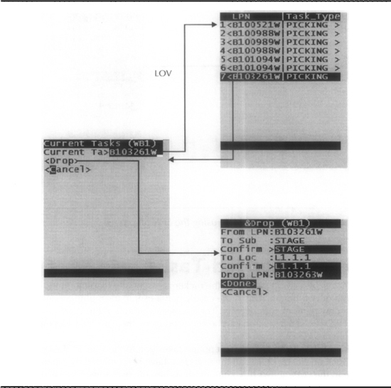
FIGURE 15-29. Users can perform multiple loads during picking and putaway and use the Current Tasks menu to drop them off

Choosing the Current Tasks menu option takes you to the Current Tasks page. The LOV for Current Tasks lists all the tasks that have been loaded by the user. The Task Type in the LOV shows the type of task. When the user selects a task, the Drop page comes up with the drop off details. The drop off subinventory and locator are displayed, and the user needs to scan these values for confirmation. If there is a discrepancy, the Reason page will pop up prompting for a reason. You can also choose a drop off LPN.

Kanban Materials Management

Kanban is a Japanese word that means “sign” or “signal.” A brief introduction to kanban was given in Chapter 1. Kanban is a self-regulating, decentralized materials management system. Kanban system is generally used for managing items that have relatively stable demand and medium to high production volume.

Interestingly enough, the inspiration behind this technique is the replenishment system used by the grocery stores in the United States. The quantity that is stored in the racks is calculated considering the forecasted demand and the replenishment interval. The racks are continuously replenished from the storage area at predetermined intervals. This section provides a detailed explanation of the features that are available in Oracle Applications to help you setup a kanban system.

Pull Sequences

Kanban items have many pull sequences that represent a series of supply points and usage points that model the actual replenishment network from the final consumption point to the original source of supply. In defining a pull sequence for a kanban item, you specify the supply source type for a kanban item at a specific location. You also specify what you want the kanban calculation program to calculate (kanban size or number of cards), the lead time for obtaining the kanban item, the allocation percentage, and other order modifiers that you want to affect the calculation program. This section discusses the concepts that are involved in a pull sequence. Defining pull sequences is covered in the section “Graphical Kanban Workbench.”

Kanban Source Types

The kanban source type identifies the type of replenishment that is required to fulfill a material requirement that is generated by a kanban. The source types supported are Production, Intra-org, Inter-org and Supplier. Figure 15-30 illustrates the different kanban source types in Oracle Applications.

FIGURE 15-30. Scenarios involving the different kanban source types

In Figure 15-30, the finished goods area stores the finished items on pallets, with a production kanban attached. When the pallet is emptied, the kanban card is sent to the assembly line. The assembly line restocks the pallet within the allowed lead time and sends it back to the finished goods area. Similarly, the assembly line sends signals to the various machining cells, for machined parts, and gets restocked. Note that the two kanbans—kanban from the finished goods area and the kanban from the assembly line—are not necessarily synchronized. That is, the assembly line doesn’t necessarily wait until it gets the kanban from the finished goods area to send its kanban to the machining cell. This might happen if the lead time allowed for the machining cell is less than the difference between the lead time allowed for the assembly cell and the lead time for assembly. For example, let’s say that the lead time allowed for the assembly cell is 36 hours per kanban quantity and the assembly lead time is 6 hours. If the machining cell needs less than 30 hours of lead time to deliver the kanban quantity required by the assembly cell, these two kanbans can be synchronized.

The assembly cell can pull purchased components from the RIP Store that serves this cell. This can either be through a backflush transaction or through an intra-org kanban. The RIP Stores can get the replenishments from the Central Store, which is an intra-org kanban. You can also communicate material requirements to other organizations or suppliers using an inter-org kanban or supplier kanban respectively.

Components of a Pull Sequence

You define a pull sequence for an item and a subinventory/locator combination. The subinventory/locator represents the usage point and is called as the kanban location. Figure 15-31 illustrates the important components of a pull sequence—usage point, supply point, and pull sequence attributes. As you can note from the figure, you should define a pull sequence for each usage point.

FIGURE 15-31. Information stored in a pull sequence

Once you identify the usage point, identify the supply point. Choose the source type from the four possible values—Intra-Org, Production, Inter-Org, or Supplier. Based on the chosen source type, you will have to provide additional information about the source type. The additional information that is applicable in each case is shown in Figure 15-31.

If the source type is production, enter the flow or discrete line that supplies to this location. If the source type is supplier, choose the supplier code and site. If you leave this blank, the requisition will be unsourced and Oracle Purchasing will attempt to find a sourcing rule for split sourcing. Sourcing rules were covered in Chapter 11. If the source type is Inter-Org, choose the organization from where you want to replenish. If the source type is Intra-Org, choose the subinventory and locator from where you want to replenish.

Once you establish the usage point and the supply point, you identify the pull sequence attributes. You can specify either kanban size or the number of cards and have the kanban planning process calculate the other. If you specify both, the kanban planning process will not plan that pull sequence. If you want the kanban size to be calculated, the number of cards is mandatory. If you want the number of cards to be calculated, the kanban size is mandatory. When you choose Do Not Calculate for the Calculate option, both kanban size and number of cards are not mandatory.

Replenishment Lead Time, Allocation Percent, Safety Stock Days, Minimum Order Quantity, and Lot Multiplier are used by the kanban planning process while calculating the kanban size. These attributes are explained in detail in the section “Kanban Planning.” If you specify the kanban size, the program will not use order modifiers to calculate the number of cards.

Kanban Sizing

Kanban size is calculated when the line is designed. Because the line is designed for the maximum rate, the kanban size is also calculated accordingly. The kanban size reflects the minimum amount of inventory that is required to support the designed daily rate. If you modify the kanban size to be lesser, you face the possibility of line shortages. Instead of reducing the kanban size, pulling a card out of the system is better. That is, make a card inactive temporarily so that it will not be used for triggering supply. Pulling out one card means you are reducing an equivalent amount of inventory from the system.

NOTE
In a kanban system, every container has a kanban that displays the item number, item description, usage point, supply point, size of the kanban (or pull quantity), and the sequence number of the card.

Accumulation of Multiple Cards

In certain scenarios, the replenishment is not effected even after a signal is received. This is especially true in the case of production kanbans that trigger production in lines that consume substantial setup time and resources. The accumulation of requirements occurs until the economic production batch size is reached. For example, the line MAC23 cannot produce the part M334533 in batch sizes that is less than 120. Several assembly lines pull this part from this machining cell in quantities of 30.

In these scenarios, accumulating the requirements and supply in batches is sensible. To aggregate demand before triggering replenishment, specify the minimum order quantity of the pull sequence to be an exact multiple of the kanban size. In the case of this example, the kanban size is 30 and the minimum order quantity is 120. The implication is that you will be accumulating four cards before triggering a supply order.

Kanban Planning

Kanban planning is a material-planning algorithm, which answers the two basic questions that any material planning algorithm tries to: When to order? and How much to order? You always reorder when your container or bin becomes empty. Every time you order, the quantity is equivalent to the kanban size. If kanban stopped here, it would have been just another material-planning algorithm. Kanban goes beyond answering these two questions and tells you how many such “kanban sizes” (in other words, cards) you need to support your material needs.

The kanban planning program doesn’t calculate both the kanban size and the number of cards for a given pull sequence. You have to specify either the kanban size or the number of cards; kanban planning will calculate the other value for you. The formula shown here is used for this calculation:

(Number of Cards –1) × Kanban Size = Average Daily Demand × (Lead Time + Safety Stock Days)

In this formula, you will provide either the number of cards or the kanban size. Figure 15-32 illustrates how the average daily demand for each item is calculated.

FIGURE 15-32. Calculating the average daily demand for an item in a location

You provide a demand source to the kanban-planning program. For a given component, the average daily demand for each of the using assembly is calculated. This average daily demand is then multiplied by the component’s quantity in the assembly to calculate the average daily demand for a component. This calculation is done based only on all the assemblies where this component has the specified kanban location as the default supply locator. In the example shown in Figure 15-32, M945980 is a component that is used by three assemblies—M342855 (Qty 2), M498903 (Qty 4), and M587393 (Qty 2). In all these three cases, the default supply locator for this component is 33-12-65. When a pull sequence is defined for M945980 with 33-12-65 as the kanban location, the average daily demand for M945980 will be 1,600.

The Allocation Percent allows you to specify the percentage of independent demand that is serviced from this kanban location. There may be many pull sequences for an item, and the planning process determines how to allocate this independent demand to these pull sequences based on the Allocation Percent. Extending the example, assume that M945980 also had an independent demand (say spare parts) of 250 from the demand source. If this particular pull sequence was defined with an Allocation Percent of 50, 125 (50 percent of 250) will be added to the dependent demand that was already calculated. So, the average daily demand for M945980 at locator 33-12-65 will be 1,725.

The replenishment lead time and safety stock days are taken from the pull sequence.

NOTE
If you want to use a kanban planning logic that is different from the one that is provided by Oracle, you have to provide the custom logic by modifying the procedure Calculate_Kanban_Quantity in the file MRPPKQCB.pls. The return values from this procedure will be checked by the kanban planning process before proceeding with the calculations using the standard formula.

An Approach to Calculating the Kanban Size

One approach to calculating the kanban size is presented in this section. The formula shown here is used for this calculation:

In this formula, the replenishment lead time in hours is divided by the replenishment hours to get the replenishment lead time in days.

Let’s take an example to understand this formula. The designed daily rate of product M345432 is 100. Component M455332 is used in the production of M345432. The required quantity is one per assembly. The lead times for replenishment are

RIP to Line: 1 Hour

Stores to RIP: 1 Day

Supplier to Stores: 5 Days

The plant operates for 20 hours in a day. Table 15-3 shows the kanban size as calculated using the kanban sizing formula for the three pull sequences.

TABLE 15-3. Kanban Size for Three Different Pull Sequences

The kanban size for RIP to Line is 5. The plant needs to build 100 assemblies per day, which translates into five per hour. Because the replenishment lead time is one hour between line and RIP stores, the hourly consumption rate itself is the kanban size.

Normally, the line has two bins to begin with, both containing components that is equivalent to the kanban quantity. The production operators pull the first bin, remove the kanban card from that bin and place it in the bin that they just consumed. This empty bin is placed in a marked place. Material handlers remove this empty bin and replenish it using the information that they find from the kanban. Thus, if you are operating a two-bin system, the number of cards that is required to support this scenario is two. This is exactly the way in which the standard formula provided by Oracle works. As you can see, when the kanban size is equal to the lead-time demand, you will be operating with two cards.

Graphical Kanban Workbench

The graphical kanban workbench allows you to perform kanban setup, kanban planning, pull sequence definition, and planning simulations through a single user interface. A graphical view of the pull sequences allows you to get the complete picture between the various points of supply and points of usage. You can mass-add pull sequences for items in the workbench. You can simulate different scenarios and update the production pull sequence from the workbench. Figure 15-33 shows the Graphical Kanban Workbench.

FIGURE 15-33. The Graphical Kanban Workbench provides a single Ul for kanban setup, kanban planning, and simulations

The workbench is comprised of two panes. The left pane displays a list of items that can be viewed by Category, Buyer Code, Planner Code, Supplier, and Location using the View By drop-down menu. There are two tabs on the left side of this pane that allow you to toggle between Production and Planning views. Once you select a view, you’ll see a list of items that are grouped according to the View By option.

Initially, the right pane displays a list of templates that can be used for creating new kanban networks. When an item is selected on the left pane, the right pane displays the data that is associated with the selected item.

The possible colors of the arrows in the replenishment chain are Black, Green, Blue, and Red. Black indicates that cards have not been generated.

Kanban Execution

Once you define the various pull sequences, you generate kanban cards and use them for managing your replenishment process. You switch the status of kanban cards between full and empty during the life cycle of a card indicating that either the kanban container is either full or needs replenishment. When the status is changed to empty, a supply order is created depending on the minimum order quantity and the type of replenishment. Sudden spikes in demand are managed by creating one-time, non-replenishable cards.

Kanban Cards

Kanban cards are based on a pull sequence and are created for a combination of item, subinventory, and locator. The card is recognized by a unique identifier. You can generate kanban cards from the pull sequence, or you may create them manually in the Kanban Cards form.

The Replenishable flag identifies if the kanban card can be replenished or if it is created for satisfying some sudden spike in demand and hence doesn’t require replenishment. Because your regular kanbans are designed for the daily rate, if you experience sudden spikes in demand, you can define non-replenishable cards to satisfy this excess demand.

You cannot override the quantity for generated cards. But you can control the inventory in the system by increasing the number of cards from the pull sequence. To reduce the inventory in the system, you can make a card inactive (covered in the “Card Status” section.)

For supplier kanbans, a supply source is defaulted if a sourcing rule is available for the item in the pull sequence. Based on the split percentage and the ranking in the sourcing rule, the primary supplier is defaulted. You can manually override this default supplier.

CAUTION
Changes to pull sequence are not reflected in the existing cards. Similarly, if you update the sourcing rule, it does not affect the existing cards. If the pull sequence is changed, you have to manually delete the existing cards and create new ones.

Card Status

The kanban card status allows you to manage the availability of the card. A card is available if the card status is Active. If you temporarily want to pull out a card from the system, set the card status to Hold. For permanently removing a card from the system, set the status to Canceled.

NOTE
Only canceled cards can be deleted.

Card Supply Status

By default, a kanban card is generated with a supply status of New. The status needs to be switched to Empty to trigger replenishment. Figure 15-34 shows the different supply statuses during the replenishment process.

FIGURE 15-34. Transition of the kanban supply status during the replenishment process

In the Figure 15-34, internal replenishment indicates intra-org and production kanbans, whereas external replenishment indicates inter-org and supplier kanbans. Once the supply status becomes Full, you can again signal replenishment by setting the card status to Empty again.

Signaling Replenishment

To signal replenishment, you set the supply status of the card to Empty. If the card is active, and if the accumulated quantity is equal to or greater than the minimum order quantity, a supply order will be created based on the supply type. There are two alternative UIs in which you can do this—the Kanban Cards form or the Replenish Kanban mobile UI. Table 15-4 explains the different supply types and what happens during the replenishment cycle of a kanban card.

TABLE 15-4. Supply Types and the Corresponding Replenishment Cycle

Kanban Cards Form

In the Kanban Cards form, set the Supply Status of the card to Empty. This will trigger the replenishment process that was illustrated in Figure 15-34.

Mobile Ul

In Oracle Mobile Materials Management, navigate to the Replenish submenu and choose Auto Replenish Kanban. In the Replenish Card Query window, scan the card number in the Card Num field. Verify that this is the card you want to replenish and select the Replenish option. If you want to cancel the transaction, select the Cancel option.

If you want to replenish multiple cards, you can enter a partial number with the standard wild card characters (_ and %), which might bring up multiple cards. In these cases, you can select the Replenish/Next option to replenish a card and bring up the next card for review.

Open Interfaces and Application Programming Interfaces

There are a number of open interfaces (Ols) and application programming interfaces (APIs) for importing data that can be processed by the various Oracle Inventory and OWM features. A list of the open interfaces and APIs are shown in Table 15-5 for reference. Please refer to the Interfaces Manual for a detailed discussion on usage.

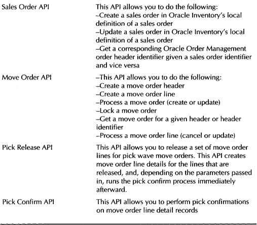
TABLE 15-5. Open Interfaces and APIs in Oracle Inventory and Oracle Warehouse Management

Summary

The various transactions in a warehouse/manufacturing plant allow you to move and store materials. Material transactions allow you to transfer materials between inventory locations. You perform material transactions using the various transactions forms or the Material Workbench.

Lots and serial numbers allow you to identify and track your materials. There are various named and user-definable attributes at the lot and serial level. You can merge and split lots, and the Lot Genealogy form allows you to view the history of these merges and splits. Serial genealogy identifies the As Built configuration of an item. Material status allows you to identify subinventories, locators, lots, and serial numbers and prevent them from certain types of transactions.

Quantity tree is a memory structure that holds the on-hand quantity information in memory. You can view the on-hand information in the Material Workbench. Reservation is the process of reserving a supply to demand. The Supply Demand form allows you to view the reservation information.

The rules framework presents a flexible way of modeling execution constraints in a warehouse. The framework consists of business objects, rules, strategies, strategy assignment to business objects, and strategy search order. There are five applications of the rules framework in OWM: picking, putaway, cost group assignment, label format, and task type assignment.

Cycle counting and physical inventory help ensure the accuracy of warehouse inventory information. The inventory planning methods Min-Max, Reorder Point, and Replenishment Counting allow you to automatically trigger replenishment orders based on predefined conditions.

OWM provides complete support for barcoding. You can minimize data entry errors due to out-of-sequence scanning using data field identifiers. The various business processes in OWM are associated with a set of label types. When the business process is executed, one label per label type is generated and can be printed using a third-party label-printing software.

Containers allow you to store and transact materials in bulk. LPNs allow you to track these containers. Cartonization is the process of generating packing configurations considering various packing constraints. You can invoke the cartonization process on pick-released items to estimate the number/type of containers that are required.

Warehouse tasks are generated and managed by the Task Type Assignment Engine and the Task Dispatching Engine. Based on the various business conditions, tasks are split and merged by these engines before being dispatched to the appropriate resource.

Materials from suppliers can be received onto the receiving dock and inspected before putaway. The putaway process invokes the rules engine to identify the best location for putaway. The opportunistic cross-docking process allows you to cross-dock material from receiving/WlP to shipping and also from receiving/WlP to WIP.

You can maintain the carrier appointments in your receiving and shipping docks using the dock calendar. Pick methodologies allow you determine how the actual picking is carried out in the warehouse. The methodologies supported are order picking, zone picking, bulk picking, and cluster picking. The wave picking process allows you to release pick waves to suit your warehouse needs. For example, you can release a pick wave that contains all the items that are contained in a particular delivery.

Picking can be executed in three modes: system directed, manual, or pick by label. The picked items can be staged in staging lanes and can then be loaded onto the carriers using the Load form. Once the items are loaded, you can perform ship confirm. The Current Tasks menu allows you to complete the tasks that were started by you and await completion.

Kanban is a pull-based materials management system. You define pull sequences that represent the network of various supply points and usage points. The kanban planning process allows you to calculate either the number of kanban cards or the kanban size. Each kanban card has various supply status, and setting this status to empty triggers the replenishment process.