
Chapter
13
Text Processing

Contents
13.1 Abundance of Digitized Text
13.1.1 Notations for Character Strings
13.2 Pattern-Matching Algorithms
13.2.2 The Boyer-Moore Algorithm
13.2.3 The Knuth-Morris-Pratt Algorithm
13.4 Text Compression and the Greedy Method
13.4.1 The Huffman Coding Algorithm
13.1 Abundance of Digitized Text
Despite the wealth of multimedia information, text processing remains one of the dominant functions of computers. Computers are used to edit, store, and display documents, and to transport files over the Internet. Furthermore, digital systems are used to archive a wide range of textual information, and new data is being generated at a rapidly increasing pace. A large corpus can readily surpass a petabyte of data (which is equivalent to a thousand terabytes, or a million gigabytes). Common examples of digital collections that include textual information are:
- Snapshots of the World Wide Web, as Internet document formats HTML and XML are primarily text formats, with added tags for multimedia content
- All documents stored locally on a user's computer
- Email archives
- Compilations of status updates on social networking sites such as Facebook
- Feeds from microblogging sites such as Twitter and Tumblr
These collections include written text from hundreds of international languages. Furthermore, there are large data sets (such as DNA) that can be viewed computationally as “strings” even though they are not language.
In this chapter, we explore some of the fundamental algorithms that can be used to efficiently analyze and process large textual data sets. In addition to having interesting applications, text-processing algorithms also highlight some important algorithmic design patterns.
We begin by examining the problem of searching for a pattern as a substring of a larger piece of text, for example, when searching for a word in a document. The pattern-matching problem gives rise to the brute-force method, which is often inefficient but has wide applicability. We continue by describing more efficient algorithms for solving the pattern-matching problem, and we examine several special-purpose data structures that can be used to better organize textual data in order to support more efficient runtime queries.
Because of the massive size of textual data sets, the issue of compression is important, both in minimizing the number of bits that need to be communicated through a network and to reduce the long-term storage requirements for archives. For text compression, we can apply the greedy method, which often allows us to approximate solutions to hard problems, and for some problems (such as in text compression) actually gives rise to optimal algorithms.
Finally, we introduce dynamic programming, an algorithmic technique that can be applied in certain settings to solve a problem in polynomial time, which appears at first to require exponential time to solve. We demonstrate the application on this technique to the problem of finding partial matches between strings that may be similar but not perfectly aligned. This problem arises when making suggestions for a misspelled word, or when trying to match related genetic samples.
13.1.1 Notations for Character Strings
When discussing algorithms for text processing, we use character strings as a model for text. Character strings can come from a wide variety of sources, including scientific, linguistic, and Internet applications. Indeed, the following are examples of such strings:
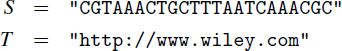
The first string, S, comes from DNA applications, and the second string, T, is the Internet address (URL) for the publisher of this book.
To allow fairly general notions of a string in our algorithm descriptions, we only assume that characters of a string come from a known alphabet, which we denote as Σ. For example, in the context of DNA, there are four symbols in the standard alphabet, Σ = {A,C,G,T}. This alphabet Σ can, of course, be a subset of the ASCII or Unicode character sets, but it could also be something more general. Although we assume that an alphabet has a fixed finite size, denoted as |Σ|, that size can be nontrivial, as with Java's treatment of the Unicode alphabet, which allows more than a million distinct characters. We therefore consider the impact of |Σ| in our asymptotic analysis of text-processing algorithms.
Java's String class provides support for representing an immutable sequence of characters, while its StringBuilder class supports mutable character sequences (see Section 1.3). For much of this chapter, we rely on the more primitive representation of a string as a char array, primarily because it allows us to use the standard indexing notation S[i], rather than the String class's more cumbersome syntax, S.charAt(i).
In order to discuss pieces of a string, we denote as a substring of an n-character string P a string of the form P[i]P[i+1]P[i+2]···P[j], for some 0 ≤ i ≤ j ≤ n − 1. To simplify the notation for referring to such substrings in prose, we let P[i..j] denote the substring of P from index i to index j inclusive. We note that string is technically a substring of itself (taking i = 0 and j = n−1), so if we want to rule this out as a possibility, we must restrict the definition to proper substrings, which require that either i > 0 or j < n − 1. We use the convention that if i > j, then P[i.. j] is equal to the null string, which has length 0.
In addition, in order to distinguish some special kinds of substrings, let us refer to any substring of the form P[0.. j], for 0 ≤ j ≤ n − 1, as a prefix of P, and any substring of the form P[i..n − 1], for 0 ≤ i ≤ n − 1, as a suffix of P. For example, if we again take P to be the string of DNA given above, then "CGTAA" is a prefix of P, "CGC" is a suffix of P, and "TTAATC" is a (proper) substring of P. Note that the null string is a prefix and a suffix of any other string.
13.2 Pattern-Matching Algorithms
In the classic pattern-matching problem, we are given a text string of length n and a pattern string of length m ≤ n, and must determine whether the pattern is a substring of the text. If so, we may want to find the lowest index within the text at which the pattern begins, or perhaps all indices at which the pattern begins.
The pattern-matching problem is inherent to many behaviors of Java's String class, such as text.contains(pattern) and text.indexOf(pattern), and is a subtask of more complex string operations such as text.replace(pattern, substitute) and text.split(pattern).
In this section, we present three pattern-matching algorithms, with increasing levels of sophistication. Our implementations report the index that begins the left-most occurrence of the pattern, if found. For a failed search, we adopt the conventions of the indexOf method of Java's String class, returning −1 as a sentinel.
13.2.1 Brute Force
The brute-force algorithmic design pattern is a powerful technique for algorithm design when we have something we wish to search for or when we wish to optimize some function. When applying this technique in a general situation, we typically enumerate all possible configurations of the inputs involved and pick the best of all these enumerated configurations.
In applying this technique to design a brute-force pattern-matching algorithm, we derive what is probably the first algorithm that we might think of for solving the problem—we simply test all the possible placements of the pattern relative to the text. An implementation of this algorithm is shown in Code Fragment 13.1.
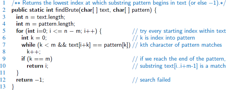
Code Fragment 13.1: An implementation of the brute-force pattern-matching algorithm. (We use character arrays rather than strings to simplify indexing notation.)
Performance
The analysis of the brute-force pattern-matching algorithm could not be simpler. It consists of two nested loops, with the outer loop indexing through all possible starting indices of the pattern in the text, and the inner loop indexing through each character of the pattern, comparing it to its potentially corresponding character in the text. Thus, the correctness of the brute-force pattern-matching algorithm follows immediately from this exhaustive search approach.
The running time of brute-force pattern matching in the worst case is not good, however, because we can perform up to m character comparisons for each candidate alignment of the pattern within the text. Referring to Code Fragment 13.1, we see that the outer for loop is executed at most n − m + 1 times, and the inner while loop is executed at most m times. Thus, the worst-case running time of the brute-force method is O(nm).
Example 13.1: Suppose we are given the text string
text = "abacaabaccabacabaabb"
and the pattern string
pattern = "abacab"
Figure 13.1 illustrates the execution of the brute-force pattern-matching algorithm on this selection of text and pattern.

Figure 13.1: Example run of the brute-force pattern-matching algorithm. The algorithm performs 27 character comparisons, indicated above with numerical labels.
13.2.2 The Boyer-Moore Algorithm
At first, it might seem that it is always necessary to examine every character in the text in order to locate a pattern as a substring or to rule out its existence. But this is not always the case. The Boyer-Moore pattern-matching algorithm, which we will study in this section, can sometimes avoid examining a significant fraction of the character in the text. In this section, we will describe a simplified version of the original algorithm by Boyer and Moore.
The main idea of the Boyer-Moore algorithm is to improve the running time of the brute-force algorithm by adding two potentially time-saving heuristics. Roughly stated, these heuristics are as follows:
Looking-Glass Heuristic: When testing a possible placement of the pattern against the text, perform the comparisons against the pattern from right-to-left.
Character-Jump Heuristic: During the testing of a possible placement of the pattern within the text, a mismatch of character text[i]=c with the corresponding character pattern[k] is handled as follows. If c is not contained anywhere in the pattern, then shift the pattern completely past text[i] = c. Otherwise, shift the pattern until an occurrence of character c gets aligned with text[i].
We will formalize these heuristics shortly, but at an intuitive level, they work as an integrated team to allow us to avoid comparisons with whole groups of characters in the text. In particular, when a mismatch is found near the right end of the pattern, we may end up realigning the pattern beyond the mismatch, without ever examining several characters of the text preceding the mismatch. For example, Figure 13.2 demonstrates a few simple applications of these heuristics. Notice that when the characters e and i mismatch at the right end of the original placement of the pattern, we slide the pattern beyond the mismatched character, without ever examining the first four characters of the text.

Figure 13.2: A simple example demonstrating the intuition of the Boyer-Moore pattern-matching algorithm. The original comparison results in a mismatch with character e of the text. Because that character is nowhere in the pattern, the entire pattern is shifted beyond its location. The second comparison is also a mismatch, but the mismatched character s occurs elsewhere in the pattern. The pattern is then shifted so that its last occurrence of s is aligned with the corresponding s in the text. The remainder of the process is not illustrated in this figure.
The example of Figure 13.2 is rather basic, because it only involves mismatches with the last character of the pattern. More generally, when a match is found for that last character, the algorithm continues by trying to extend the match with the second-to-last character of the pattern in its current alignment. That process continues until either matching the entire pattern, or finding a mismatch at some interior position of the pattern.
If a mismatch is found, and the mismatched character of the text does not occur in the pattern, we shift the entire pattern beyond that location, as originally illustrated in Figure 13.2. If the mismatched character occurs elsewhere in the pattern, we must consider two possible subcases depending on whether its last occurrence is before or after the character of the pattern that was mismatched. Those two cases are illustrated in Figure 13.3.
In the case of Figure 13.3(b), we slide the pattern only one unit. It would be more productive to slide it rightward until finding another occurrence of mismatched character text[i] in the pattern, but we do not wish to take time to search for another occurrence. The efficiency of the Boyer-Moore algorithm relies on quickly determining where a mismatched character occurs elsewhere in the pattern. In particular, we define a function last(c) as
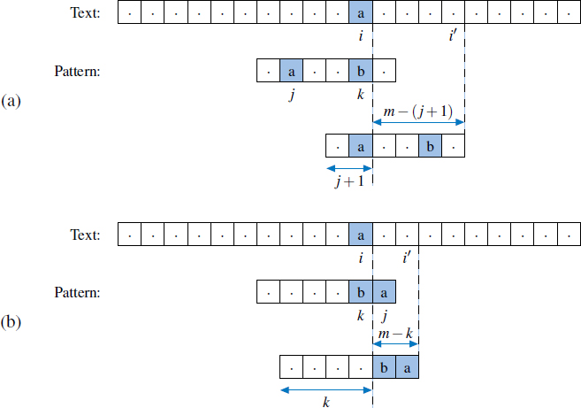
Figure 13.3: Additional rules for the character-jump heuristic of the Boyer-Moore algorithm. We let i represent the index of the mismatched character in the text, k represent the corresponding index in the pattern, and j represent the index of the last occurrence of text[i] within the pattern. We distinguish two cases: (a) j < k, in which case we shift the pattern by k − j units, and thus, index i advances by m − (j + 1) units; (b) j > k, in which case we shift the pattern by one unit, and index i advances by m − k units.
- If c is in the pattern, last(c) is the index of the last (rightmost) occurrence of c in the pattern. Otherwise, we conventionally define last(c) = −1.
If we assume that the alphabet is of fixed, finite size, and that characters can be converted to indices of an array (for example, by using their character code), the last function can be easily implemented as a lookup table with worst-case O(1)-time access to the value last(c). However, the table would have length equal to the size of the alphabet (rather than the size of the pattern), and time would be required to initialize the entire table.
We prefer to use a hash table to represent the last function, with only those characters from the pattern occurring in the map. The space usage for this approach is proportional to the number of distinct alphabet symbols that occur in the pattern, and thus O(max(m, |Σ|)). The expected lookup time remains O(1) (as does the worst-case, if we consider |Σ| a constant). Our complete implementation of the Boyer-Moore pattern-matching algorithm is given in Code Fragment 13.2.
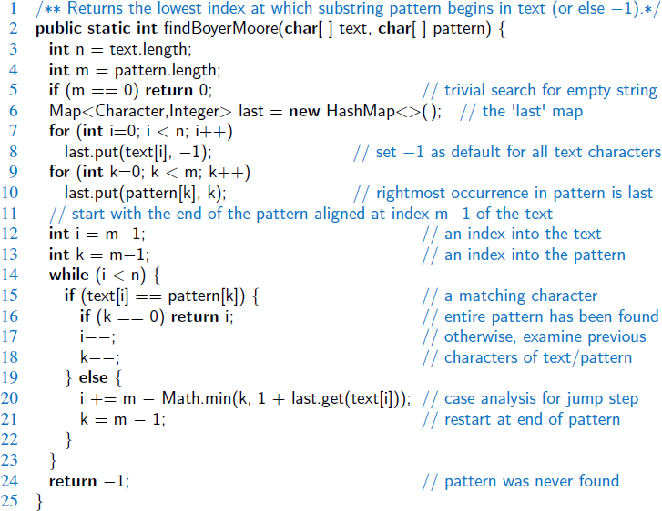
Code Fragment 13.2: An implementation of the Boyer-Moore algorithm.
The correctness of the Boyer-Moore pattern-matching algorithm follows from the fact that each time the method makes a shift, it is guaranteed not to “skip” over any possible matches. For last(c) is the location of the last occurrence of c in the pattern. In Figure 13.4, we illustrate the execution of the Boyer-Moore pattern-matching algorithm on an input string similar to Example 13.1.

Figure 13.4: An illustration of the Boyer-Moore pattern-matching algorithm, including a summary of the last(c) function. The algorithm performs 13 character comparisons, which are indicated with numerical labels.
Performance
If using a traditional lookup table, the worst-case running time of the Boyer-Moore algorithm is O(nm + |Σ|). The computation of the last function takes O(m+|Σ|) time, although the dependence on |Σ| is removed if using a hash table. The actual search for the pattern takes O(nm) time in the worst case—the same as the brute-force algorithm. An example that achieves the worst case for Boyer-Moore is

The worst-case performance, however, is unlikely to be achieved for English text; in that case, the Boyer-Moore algorithm is often able to skip large portions of text. Experimental evidence on English text shows that the average number of comparisons done per character is 0.24 for a five-character pattern string.
We have actually presented a simplified version of the Boyer-Moore algorithm. The original algorithm achieves worst-case running time O(n + m + |Σ|) by using an alternative shift heuristic for a partially matched text string, whenever it shifts the pattern more than the character-jump heuristic. This alternative shift heuristic is based on applying the main idea from the Knuth-Morris-Pratt pattern-matching algorithm, which we discuss next.
13.2.3 The Knuth-Morris-Pratt Algorithm
In examining the worst-case performances of the brute-force and Boyer-Moore pattern-matching algorithms on specific instances of the problem, such as that given in Example 13.1, we should notice a major inefficiency (at least in the worst case). For a certain alignment of the pattern, if we find several matching characters but then detect a mismatch, we ignore all the information gained by the successful comparisons after restarting with the next incremental placement of the pattern.
The Knuth-Morris-Pratt (or “KMP”) algorithm, discussed in this section, avoids this waste of information and, in so doing, it achieves a running time of O(n + m), which is asymptotically optimal. That is, in the worst case any pattern-matching algorithm will have to examine all the characters of the text and all the characters of the pattern at least once. The main idea of the KMP algorithm is to precompute self-overlaps between portions of the pattern so that when a mismatch occurs at one location, we immediately know the maximum amount to shift the pattern before continuing the search. A motivating example is shown in Figure 13.5.

Figure 13.5: A motivating example for the Knuth-Morris-Pratt algorithm. If a mismatch occurs at the indicated location, the pattern could be shifted to the second alignment, without explicit need to recheck the partial match with the prefix ama. If the mismatched character is not an l, then the next potential alignment of the pattern can take advantage of the common a.
The Failure Function
To implement the KMP algorithm, we will precompute a failure function, f, that indicates the proper shift of the pattern upon a failed comparison. Specifically, the failure function f(k) is defined as the length of the longest prefix of the pattern that is a suffix of the substring pattern[1..k] (note that we did not include pattern[0] here, since we will shift at least one unit). Intuitively, if we find a mismatch upon character pattern[k+1], the function f(k) tells us how many of the immediately preceding characters can be reused to restart the pattern. Example 13.2 describes the value of the failure function for the example pattern from Figure 13.5.
Example 13.2: Consider the pattern “amalgamation” from Figure 13.5. The Knuth-Morris-Pratt (KMP) failure function, f(k), for the string P is as shown in the following table:

Implementation
Our implementation of the KMP pattern-matching algorithm is shown in Code Fragment 13.3. It relies on a utility method, computeFailKMP, discussed on the next page, to compute the failure function efficiently.
The main part of the KMP algorithm is its while loop, each iteration of which performs a comparison between the character at index j in the text and the character at index k in the pattern. If the outcome of this comparison is a match, the algorithm moves on to the next characters in both (or reports a match if reaching the end of the pattern). If the comparison failed, the algorithm consults the failure function for a new candidate character in the pattern, or starts over with the next index in the text if failing on the first character of the pattern (since nothing can be reused).

Code Fragment 13.3: An implementation of the KMP pattern-matching algorithm. The computeFailKMP utility method is given in Code Fragment 13.4.
Constructing the KMP Failure Function
To construct the failure function, we use the method shown in Code Fragment 13.4, which is a “bootstrapping” process that compares the pattern to itself as in the KMP algorithm. Each time we have two characters that match, we set f(j) = k + 1. Note that since we have j > k throughout the execution of the algorithm, f(k − 1) is always well defined when we need to use it.
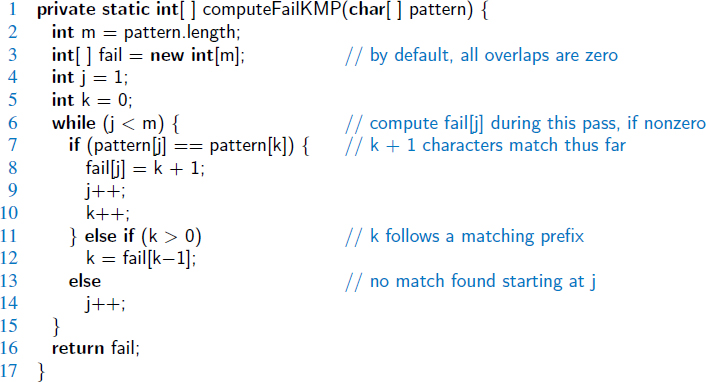
Code Fragment 13.4: An implementation of the computeFailKMP utility in support of the KMP pattern-matching algorithm. Note how the algorithm uses the previous values of the failure function to efficiently compute new values.
Performance
Excluding the computation of the failure function, the running time of the KMP algorithm is clearly proportional to the number of iterations of the while loop. For the sake of the analysis, let us define s = j − k. Intuitively, s is the total amount by which the pattern has been shifted with respect to the text. Note that throughout the execution of the algorithm, we have s ≤ n. One of the following three cases occurs at each iteration of the loop.
- If text[j] = pattern[k], then j and k each increase by 1, thus s is unchanged.
- If text[j] ≠ pattern[k] and k > 0, then j does not change and s increases by at least 1, since in this case s changes from j−k to j−f(k−1); note that this is an addition of k − f(k − 1), which is positive because f(k−1) < k.
- If text[j] ≠ pattern[k] and k = 0, then j increases by 1 and s increases by 1, since k does not change.
Thus, at each iteration of the loop, either j or s increases by at least 1 (possibly both); hence, the total number of iterations of the while loop in the KMP pattern-matching algorithm is at most 2n. Achieving this bound, of course, assumes that we have already computed the failure function for the pattern.
The algorithm for computing the failure function runs in O(m) time. Its analysis is analogous to that of the main KMP algorithm, yet with a pattern of length m compared to itself. Thus, we have:
Proposition 13.3: The Knuth-Morris-Pratt algorithm performs pattern matching on a text string of length n and a pattern string of length m in O(n+m) time.
The correctness of this algorithm follows from the definition of the failure function. Any comparisons that are skipped are actually unnecessary, for the failure function guarantees that all the ignored comparisons are redundant—they would involve comparing the same matching characters over again.
In Figure 13.6, we illustrate the execution of the KMP pattern-matching algorithm on the same input strings as in Example 13.1. Note the use of the failure function to avoid redoing one of the comparisons between a character of the pattern and a character of the text. Also note that the algorithm performs fewer overall comparisons than the brute-force algorithm run on the same strings (Figure 13.1).

Figure 13.6: An illustration of the KMP pattern-matching algorithm. The primary algorithm performs 19 character comparisons, which are indicated with numerical labels. (Additional comparisons would be performed during the computation of the failure function.)
13.3 Tries
The pattern-matching algorithms presented in Section 13.2 speed up the search in a text by preprocessing the pattern (to compute the last function in the Boyer-Moore algorithm or the failure function in the Knuth-Morris-Pratt algorithm). In this section, we take a complementary approach, namely, we present string searching algorithms that preprocess the text, rather than the pattern. This approach is suitable for applications in which many queries are performed on a fixed text, so that the initial cost of preprocessing the text is compensated by a speedup in each subsequent query (for example, a website that offers pattern matching in Shakespeare's Hamlet or a search engine that offers Web pages containing the term Hamlet).
A trie (pronounced “try”) is a tree-based data structure for storing strings in order to support fast pattern matching. The main application for tries is in information retrieval. Indeed, the name “trie” comes from the word “retrieval.” In an information retrieval application, such as a search for a certain DNA sequence in a genomic database, we are given a collection S of strings, all defined using the same alphabet. The primary query operations that tries support are pattern matching and prefix matching. The latter operation involves being given a string X, and looking for all the strings in S that being with X.
13.3.1 Standard Tries
Let S be a set of s strings from alphabet Σ such that no string in S is a prefix of another string. A standard trie for S is an ordered tree T with the following properties (see Figure 13.7):
- Each node of T, except the root, is labeled with a character of Σ.
- The children of an internal node of T have distinct labels.
- T has s leaves, each associated with a string of S, such that the concatenation of the labels of the nodes on the path from the root to a leaf v of T yields the string of S associated with v.
Thus, a trie T represents the strings of S with paths from the root to the leaves of T. Note the importance of assuming that no string in S is a prefix of another string. This ensures that each string of S is uniquely associated with a leaf of T. (This is similar to the restriction for prefix codes with Huffman coding, as described in Section 13.4.) We can always satisfy this assumption by adding a special character that is not in the original alphabet Σ at the end of each string.
An internal node in a standard trie T can have anywhere between 1 and |Σ| children. There is an edge going from the root r to one of its children for each character that is first in some string in the collection S. In addition, a path from the root of T to an internal node v at depth k corresponds to a k-character prefix X[0..k − 1] of a string X of S. In fact, for each character c that can follow the prefix X[0..k − 1] in a string of the set S, there is a child of v labeled with character c. In this way, a trie concisely stores the common prefixes that exist among a set of strings.

Figure 13.7: Standard trie for the strings {bear, bell, bid, bull, buy, sell, stock, stop}.
As a special case, if there are only two characters in the alphabet, then the trie is essentially a binary tree, with some internal nodes possibly having only one child (that is, it may be an improper binary tree). In general, although it is possible that an internal node has up to |Σ| children, in practice the average degree of such nodes is likely to be much smaller. For example, the trie shown in Figure 13.7 has several internal nodes with only one child. On larger data sets, the average degree of nodes is likely to get smaller at greater depths of the tree, because there may be fewer strings sharing the common prefix, and thus fewer continuations of that pattern. Furthermore, in many languages, there will be character combinations that are unlikely to naturally occur.
The following proposition provides some important structural properties of a standard trie:
Proposition 13.4: A standard trie storing a collection S of s strings of total length n from an alphabet Σ has the following properties:
- The height of T is equal to the length of the longest string in S.
- Every internal node of T has at most |Σ| children.
- T has s leaves.
- The number of nodes of T is at most n + 1.
The worst case for the number of nodes of a trie occurs when no two strings share a common nonempty prefix; that is, except for the root, all internal nodes have one child.
A trie T for a set S of strings can be used to implement a set or map whose keys are the strings of S. Namely, we perform a search in T for a string X by tracing down from the root the path indicated by the characters in X. If this path can be traced and terminates at a leaf node, then we know X is a string in S. For example, in the trie in Figure 13.7, tracing the path for “bull” ends up at a leaf. If the path cannot be traced or the path can be traced but terminates at an internal node, then X is not a string in S. In the example in Figure 13.7, the path for “bet” cannot be traced and the path for “be” ends at an internal node. Neither such word is in the set S.
It is easy to see that the running time of the search for a string of length m is O(m · |Σ|), because we visit at most m+1 nodes of T and we spend O(|Σ|) time at each node determining the child having the subsequent character as a label. The O(|Σ|) upper bound on the time to locate a child with a given label is achievable, even if the children of a node are unordered, since there are at most |Σ| children. We can improve the time spent at a node to be O(log|Σ|) or expected O(1), by mapping characters to children using a secondary search table or hash table at each node, or by using a direct lookup table of size |Σ| at each node, if |Σ| is sufficiently small (as is the case for DNA strings). For these reasons, we typically expect a search for a string of length m to run in O(m) time.
From the discussion above, it follows that we can use a trie to perform a special type of pattern matching, called word matching, where we want to determine whether a given pattern matches one of the words of the text exactly. Word matching differs from standard pattern matching because the pattern cannot match an arbitrary substring of the text—only one of its words. To accomplish this, each word of the original document must be added to the trie. (See Figure 13.8.) A simple extension of this scheme supports prefix-matching queries. However, arbitrary occurrences of the pattern in the text (for example, the pattern is a proper suffix of a word or spans two words) cannot be efficiently performed.
To construct a standard trie for a set S of strings, we can use an incremental algorithm that inserts the strings one at a time. Recall the assumption that no string of S is a prefix of another string. To insert a string X into the current trie T, we trace the path associated with X in T, creating a new chain of nodes to store the remaining characters of X when we get stuck. The running time to insert X with length m is similar to a search, with worst-case O(m·|Σ|) performance, or expected O(m) if using secondary hash tables at each node. Thus, constructing the entire trie for set S takes expected O(n) time, where n is the total length of the strings of S.
There is a potential space inefficiency in the standard trie that has prompted the development of the compressed trie, which is also known (for historical reasons) as the Patricia trie. Namely, there are potentially a lot of nodes in the standard trie that have only one child, and the existence of such nodes is a waste. We discuss the compressed trie next.

Figure 13.8: Word matching with a standard trie: (a) text to be searched (articles and prepositions, which are also known as stop words, excluded); (b) standard trie for the words in the text, with leaves augmented with indications of the index at which the given work begins in the text. For example, the leaf for the word “stock” notes that the word begins at indices 17, 40, 51, and 62 of the text.
13.3.2 Compressed Tries
A compressed trie is similar to a standard trie but it ensures that each internal node in the trie has at least two children. It enforces this rule by compressing chains of single-child nodes into individual edges. (See Figure 13.9.) Let T be a standard trie. We say that an internal node v of T is redundant if v has one child and is not the root. For example, the trie of Figure 13.7 has eight redundant nodes. Let us also say that a chain of k ≥ 2 edges,
(v0, v1)(v1, v2) ···(vk−1, vk),
is redundant if:
- vi is redundant for i = 1, ..., k − 1.
- v0 and vk are not redundant.
We can transform T into a compressed trie by replacing each redundant chain (v0, v1)...(vk−1, vk) of k ≥ 2 edges into a single edge (v0, vk), relabeling vk with the concatenation of the labels of nodes v1,...,vk.

Figure 13.9: Compressed trie for the strings {bear, bell, bid, bull, buy, sell, stock, stop}. (Compare this with the standard trie shown in Figure 13.7.) Notice that, in addition to compression at the leaves, the internal node with label “to” is shared by words “stock” and “stop”.
Thus, nodes in a compressed trie are labeled with strings, which are substrings of strings in the collection, rather than with individual characters. The advantage of a compressed trie over a standard trie is that the number of nodes of the compressed trie is proportional to the number of strings and not to their total length, as shown in the following proposition (compare with Proposition 13.4).
Proposition 13.5: A compressed trie storing a collection S of s strings from an alphabet of size d has the following properties:
- Every internal node of T has at least two children and most d children.
- T has s leaves nodes.
- The number of nodes of T is O(s).
The attentive reader may wonder whether the compression of paths provides any significant advantage, since it is offset by a corresponding expansion of the node labels. Indeed, a compressed trie is truly advantageous only when it is used as an auxiliary index structure over a collection of strings already stored in a primary structure, and is not required to actually store all the characters of the strings in the collection.
Suppose, for example, that the collection S of strings is an array of strings S[0], S[1], ..., S[s−1]. Instead of storing the label X of a node explicitly, we represent it implicitly by a combination of three integers (i, j, k), such that X = S[i][j..k]; that is, X is the substring of S[i] consisting of the characters from the jth to the kth inclusive. (See the example in Figure 13.10. Also compare with the standard trie of Figure 13.8.)

Figure 13.10: (a) Collection S of strings stored in an array. (b) Compact representation of the compressed trie for S.
This additional compression scheme allows us to reduce the total space for the trie itself from O(n) for the standard trie to O(s) for the compressed trie, where n is the total length of the strings in S and s is the number of strings in S. We must still store the different strings in S, of course, but we nevertheless reduce the space for the trie.
Searching in a compressed trie is not necessarily faster than in a standard tree, since there is still need to compare every character of the desired pattern with the potentially multicharacter labels while traversing paths in the trie.
13.3.3 Suffix Tries
One of the primary applications for tries is for the case when the strings in the collection S are all the suffixes of a string X. Such a trie is called the suffix trie (also known as a suffix tree or position tree) of string X. For example, Figure 13.11a shows the suffix trie for the eight suffixes of string “minimize.” For a suffix trie, the compact representation presented in the previous section can be further simplified. Namely, the label of each vertex is a pair “j..k” indicating the string X[j..k]. (See Figure 13.11b.) To satisfy the rule that no suffix of X is a prefix of another suffix, we can add a special character, denoted with $, that is not in the original alphabet Σ at the end of X (and thus to every suffix). That is, if string X has length n, we build a trie for the set of n strings X[ j..n−1]$, for j = 0,...,n − 1.
Saving Space
Using a suffix trie allows us to save space over a standard trie by using several space compression techniques, including those used for the compressed trie.
The advantage of the compact representation of tries now becomes apparent for suffix tries. Since the total length of the suffixes of a string X of length n is
![]()
storing all the suffixes of X explicitly would take O(n2) space. Even so, the suffix trie represents these strings implicitly in O(n) space, as formally stated in the following proposition.
Proposition 13.6: The compact representation of a suffix trie T for a string X of length n uses O(n) space.
Construction
We can construct the suffix trie for a string of length n with an incremental algorithm like the one given in Section 13.3.1. This construction takes O(|Σ|n2) time because the total length of the suffixes is quadratic in n. However, the (compact) suffix trie for a string of length n can be constructed in O(n) time with a specialized algorithm, different from the one for general tries. This linear-time construction algorithm is fairly complex, however, and is not reported here. Still, we can take advantage of the existence of this fast construction algorithm when we want to use a suffix trie to solve other problems.

Figure 13.11: (a) Suffix trie T for the string X = "minimize". (b) Compact representation of T, where pair j..k denotes the substring X[j..k] in the reference string.
Using a Suffix Trie
The suffix trie T for a string X can be used to efficiently perform pattern-matching queries on text X. Namely, we can determine whether a pattern is a substring of X by trying to trace a path associated with P in T. P is a substring of X if and only if such a path can be traced. The search down the trie T assumes that nodes in T store some additional information, with respect to the compact representation of the suffix trie:
If node v has label j..k and Y is the string of length y associated with the path from the root to v (included), then X[k − y + 1..k] = Y.
This property ensures that we can compute the start index of the pattern in the text when a match occurs in O(m) time.
13.3.4 Search Engine Indexing
The World Wide Web contains a huge collection of text documents (Web pages). Information about these pages are gathered by a program called a Web crawler, which then stores this information in a special dictionary database. A Web search engine allows users to retrieve relevant information from this database, thereby identifying relevant pages on the Web containing given keywords. In this section, we will present a simplified model of a search engine.
Inverted Files
The core information stored by a search engine is a map, called an inverted index or inverted file, storing key-value pairs (w,L), where w is a word and L is a collection of pages containing word w. The keys (words) in this map are called index terms and should be a set of vocabulary entries and proper nouns as large as possible. The values in this map are called occurrence lists and should cover as many Web pages as possible.
We can efficiently implement an inverted index with a data structure consisting of the following:
- An array storing the occurrence lists of the terms (in no particular order).
- A compressed trie for the set of index terms, where each leaf stores the index of the occurrence list of the associated term.
The reason for storing the occurrence lists outside the trie is to keep the size of the trie data structure sufficiently small to fit in internal memory. Instead, because of their large total size, the occurrence lists have to be stored on disk.
With our data structure, a query for a single keyword is similar to a word-matching query (Section 13.3.1). Namely, we find the keyword in the trie and we return the associated occurrence list.
When multiple keywords are given and the desired output are the pages containing all the given keywords, we retrieve the occurrence list of each keyword using the trie and return their intersection. To facilitate the intersection computation, each occurrence list should be implemented with a sequence sorted by address or with a map, to allow efficient set operations.
In addition to the basic task of returning a list of pages containing given keywords, search engines provide an important additional service by ranking the pages returned by relevance. Devising fast and accurate ranking algorithms for search engines is a major challenge for computer researchers and electronic commerce companies.
13.4 Text Compression and the Greedy Method
In this section, we will consider the important task of text compression. In this problem, we are given a string X defined over some alphabet, such as the ASCII or Unicode character sets, and we want to efficiently encode X into a small binary string Y (using only the characters 0 and 1). Text compression is useful in any situation where we wish to reduce bandwidth for digital communications, so as to minimize the time needed to transmit our text. Likewise, text compression is useful for storing large documents more efficiently, so as to allow a fixed-capacity storage device to contain as many documents as possible.
The method for text compression explored in this section is the Huffman code. Standard encoding schemes, such as ASCII, use fixed-length binary strings to encode characters (with 7 or 8 bits in the traditional or extended ASCII systems, respectively). The Unicode system was originally proposed as a 16-bit fixed-length representation, although common encodings reduce the space usage by allowing common groups of characters, such as those from the ASCII system, with fewer bits. The Huffman code saves space over a fixed-length encoding by using short code-word strings to encode high-frequency characters and long code-word strings to encode low-frequency characters. Furthermore, the Huffman code uses a variable-length encoding specifically optimized for a given string X over any alphabet. The optimization is based on the use of character frequencies, where we have, for each character c, a count f(c) of the number of times c appears in the string X.
To encode the string X, we convert each character in X to a variable-length code-word, and we concatenate all these code-words in order to produce the encoding Y for X. In order to avoid ambiguities, we insist that no code-word in our encoding be a prefix of another code-word in our encoding. Such a code is called a prefix code, and it simplifies the decoding of Y to retrieve X. (See Figure 13.12.) Even with this restriction, the savings produced by a variable-length prefix code can be significant, particularly if there is a wide variance in character frequencies (as is the case for natural language text in almost every written language).
Huffman's algorithm for producing an optimal variable-length prefix code for X is based on the construction of a binary tree T that represents the code. Each edge in T represents a bit in a code-word, with an edge to a left child representing a “0” and an edge to a right child representing a “1”. Each leaf v is associated with a specific character, and the code-word for that character is defined by the sequence of bits associated with the edges in the path from the root of T to v. (See Figure 13.12.) Each leaf v has a frequency, f(v), which is simply the frequency in X of the character associated with v. In addition, we give each internal node v in T a frequency, f(v), that is the sum of the frequencies of all the leaves in the subtree rooted at v.

Figure 13.12: An illustration of an example Huffman code for the input string X = "a fast runner need never be afraid of the dark": (a) frequency of each character of X; (b) Huffman tree T for string X. The code for a character c is obtained by tracing the path from the root of T to the leaf where c is stored, and associating a left child with 0 and a right child with 1. For example, the code for "r" is 011, and the code for "h" is 10111.
13.4.1 The Huffman Coding Algorithm
The Huffman coding algorithm begins with each of the d distinct characters of the string X to encode being the root node of a single-node binary tree. The algorithm proceeds in a series of rounds. In each round, the algorithm takes the two binary trees with the smallest frequencies and merges them into a single binary tree. It repeats this process until only one tree is left. (See Code Fragment 13.5.)
Each iteration of the while loop in Huffman's algorithm can be implemented in O(logd) time using a priority queue represented with a heap. In addition, each iteration takes two nodes out of Q and adds one in, a process that will be repeated d−1 times before exactly one node is left in Q. Thus, this algorithm runs in O(n+d logd) time. Although a full justification of this algorithm's correctness is beyond our scope here, we note that its intuition comes from a simple idea—any optimal code can be converted into an optimal code in which the code-words for the two lowest-frequency characters, a and b, differ only in their last bit. Repeating the argument for a string with a and b replaced by a character c, gives the following:
Proposition 13.7: Huffman's algorithm constructs an optimal prefix code for a string of length n with d distinct characters in O(n + d logd) time.

Code Fragment 13.5: Huffman coding algorithm.
13.4.2 The Greedy Method
Huffman's algorithm for building an optimal encoding is an example application of an algorithmic design pattern called the greedy method. This design pattern is applied to optimization problems, where we are trying to construct some structure while minimizing or maximizing some property of that structure.
The general formula for the greedy-method pattern is almost as simple as that for the brute-force method. In order to solve a given optimization problem using the greedy method, we proceed by a sequence of choices. The sequence starts from some well-understood starting condition, and computes the cost for that initial condition. The pattern then asks that we iteratively make additional choices by identifying the decision that achieves the best cost improvement from all of the choices that are currently possible. This approach does not always lead to an optimal solution.
But there are several problems that it does work for, and such problems are said to possess the greedy-choice property. This is the property that a global optimal condition can be reached by a series of locally optimal choices (that is, choices that are each the current best from among the possibilities available at the time), starting from a well-defined starting condition. The problem of computing an optimal variable-length prefix code is just one example of a problem that possesses the greedy-choice property.
13.5 Dynamic Programming
In this section, we will discuss the dynamic-programming algorithmic design pattern. This technique is similar to the divide-and-conquer technique (Section 12.1.1), in that it can be applied to a wide variety of different problems. Dynamic programming can often be used to produce polynomial-time algorithms to solve problems that seem to require exponential time. In addition, the algorithms that result from applications of the dynamic programming technique are usually quite simple, often needing little more than a few lines of code to describe some nested loops for filling in a table.
13.5.1 Matrix Chain-Product
Rather than starting out with an explanation of the general components of the dynamic programming technique, we begin by giving a classic, concrete example. Suppose we are given a collection of n two-dimensional matrices for which we wish to compute the mathematical product
A = A0 · A1 · A2 ... An−1,
where Ai is a di × di+1 matrix, for i = 0, 1, 2,...,n − 1. In the standard matrix multiplication algorithm (which is the one we will use), to multiply a d×e-matrix B times an e × f-matrix C, we compute the product, A, as

This definition implies that matrix multiplication is associative, that is, it implies that B · (C · D) = (B · C) · D. Thus, we can parenthesize the expression for A any way we wish and we will end up with the same answer. However, we will not necessarily perform the same number of primitive (that is, scalar) multiplications in each parenthesization, as is illustrated in the following example.
Example 13.8: Let B be a 2 × 10-matrix, let C be a 10 × 50-matrix, and let D be a 50×20-matrix. Computing B · (C · D) requires 2 · 10 · 20 + 10 · 50 · 20 = 10400 multiplications, whereas computing (B·C) · D requires 2·10·50+2·50·20 =3000 multiplications.
The matrix chain-product problem is to determine the parenthesization of the expression defining the product A that minimizes the total number of scalar multiplications performed. As the example above illustrates, the differences between parenthesizations can be dramatic, so finding a good solution can result in significant speedups.
Defining Subproblems
One way to solve the matrix chain-product problem is to simply enumerate all the possible ways of parenthesizing the expression for A and determine the number of multiplications performed by each one. Unfortunately, the set of all different parenthesizations of the expression for A is equal in number to the set of all different binary trees that have n leaves. This number is exponential in n. Thus, this straightforward (“brute-force”) algorithm runs in exponential time, for there are an exponential number of ways to parenthesize an associative arithmetic expression.
We can significantly improve the performance achieved by the brute-force algorithm, however, by making a few observations about the nature of the matrix chain-product problem. The first is that the problem can be split into subproblems. In this case, we can define a number of different subproblems, each of which is to compute the best parenthesization for some subexpression Ai · Ai+1 ... Aj. As a concise notation, we use Ni,j to denote the minimum number of multiplications needed to compute this subexpression. Thus, the original matrix chain-product problem can be characterized as that of computing the value of N0,n−1. This observation is important, but we need one more in order to apply the dynamic programming technique.
Characterizing Optimal Solutions
The other important observation we can make about the matrix chain-product problem is that it is possible to characterize an optimal solution to a particular subproblem in terms of optimal solutions to its subproblems. We call this property the subproblem optimality condition.
In the case of the matrix chain-product problem, we observe that, no matter how we parenthesize a subexpression, there has to be some final matrix multiplication that we perform. That is, a full parenthesization of a subexpression Ai · Ai+1 ... Aj has to be of the form (Ai ... Ak) · (Ak+1 ... Aj), for some k ∈ {i, i+1, ..., j − 1}. Moreover, for whichever k is the correct one, the products (Ai...Ak) and (Ak+1 ... Aj) must also be solved optimally. If this were not so, then there would be a global optimal that had one of these subproblems solved suboptimally. But this is impossible, since we could then reduce the total number of multiplications by replacing the current subproblem solution by an optimal solution for the subproblem. This observation implies a way of explicitly defining the optimization problem for Ni, j in terms of other optimal subproblem solutions. Namely, we can compute Ni, j by considering each place k where we could put the final multiplication and taking the minimum over all such choices.
Designing a Dynamic Programming Algorithm
We can therefore characterize the optimal subproblem solution, Ni, j, as
![]()
where Ni,i = 0, since no work is needed for a single matrix. That is, Ni, j is the minimum, taken over all possible places to perform the final multiplication, of the number of multiplications needed to compute each subexpression plus the number of multiplications needed to perform the final matrix multiplication.
Notice that there is a sharing of subproblems going on that prevents us from dividing the problem into completely independent subproblems (as we would need to do to apply the divide-and-conquer technique). We can, nevertheless, use the equation for Ni, j to derive an efficient algorithm by computing Ni, j values in a bottom-up fashion, and storing intermediate solutions in a table of Ni, j values. We can begin simply enough by assigning Ni,i = 0 for i = 0,1,...,n−1. We can then apply the general equation for Ni, j to compute Ni,i+1 values, since they depend only on Ni,i and Ni+1,i+1 values that are available. Given the Ni,i+1 values, we can then compute the Ni,i+2 values, and so on. Therefore, we can build Ni, j values up from previously computed values until we can finally compute the value of N0,n−1, which is the number that we are searching for. A Java implementation of this dynamic programming solution is given in Code Fragment 13.6; we use techniques from Section 3.1.5 for working with a two-dimensional array in Java.
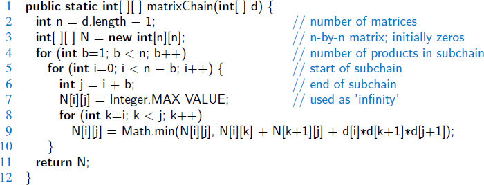
Code Fragment 13.6: Dynamic programming algorithm for the matrix chain-product problem.
Thus, we can compute N0,n−1 with an algorithm that consists primarily of three nested loops (the third of which computes the min term). Each of these loops iterates at most n times per execution, with a constant amount of additional work within. Therefore, the total running time of this algorithm is O(n3).
13.5.2 DNA and Text Sequence Alignment
A common text-processing problem, which arises in genetics and software engineering, is to test the similarity between two text strings. In a genetics application, the two strings could correspond to two strands of DNA, for which we want to compute similarities. Likewise, in a software engineering application, the two strings could come from two versions of source code for the same program, for which we want to determine changes made from one version to the next. Indeed, determining the similarity between two strings is so common that the Unix and Linux operating systems have a built-in program, named diff, for comparing text files.
Given a string X = x0x1x2 ... xn−1, a subsequence of X is any string that is of the form xi1xi2 ... xik, where ij < ij+1; that is, it is a sequence of characters that are not necessarily contiguous but are nevertheless taken in order from X. For example, the string AAAG is a subsequence of the string CGATAATTGAGA.
The DNA and text similarity problem we address here is the longest common subsequence (LCS) problem. In this problem, we are given two character strings, X = x0x1x2...xn−1 and Y = y0y1y2...ym−1, over some alphabet (such as the alphabet {A,C,G,T} common in computational genomics) and are asked to find a longest string S that is a subsequence of both X and Y. One way to solve the longest common subsequence problem is to enumerate all subsequences of X and take the largest one that is also a subsequence of Y. Since each character of X is either in or not in a subsequence, there are potentially 2n different subsequences of X, each of which requires O(m) time to determine whether it is a subsequence of Y. Thus, this brute-force approach yields an exponential-time algorithm that runs in O(2nm) time, which is very inefficient. Fortunately, the LCS problem is efficiently solvable using dynamic programming.
The Components of a Dynamic Programming Solution
As mentioned above, the dynamic programming technique is used primarily for optimization problems, where we wish to find the “best” way of doing something. We can apply the dynamic programming technique in such situations if the problem has certain properties:
Simple Subproblems: There has to be some way of repeatedly breaking the global optimization problem into subproblems. Moreover, there should be a way to parameterize subproblems with just a few indices, like i, j, k, and so on.
Subproblem Optimization: An optimal solution to the global problem must be a composition of optimal subproblem solutions.
Subproblem Overlap: Optimal solutions to unrelated subproblems can contain subproblems in common.
Applying Dynamic Programming to the LCS Problem
Recall that in the LCS problem, we are given two character strings, X and Y, of length n and m, respectively, and are asked to find a longest string S that is a subsequence of both X and Y. Since X and Y are character strings, we have a natural set of indices with which to define subproblems—indices into the strings X and Y. Let us define a subproblem, therefore, as that of computing the value Lj,k, which we will use to denote the length of a longest string that is a subsequence of both the first j characters of X and the first k characters of Y, that is of prefixes X[0.. j − 1] and Y[0..k − 1]. If either j = 0 or k = 0, then Lj,k is trivially defined as 0.
When both j ≥ 1 and k ≥ 1, this definition allows us to rewrite Lj,k recursively in terms of optimal subproblem solutions. This definition depends on which of two cases we are in. (See Figure 13.13.)
- xj−1 = yk−1. In this case, we have a match between the last character of X[0.. j−1] and the last character of Y[0..k−1]. We claim that this character belongs to a longest common subsequence of X[0.. j − 1] and Y[0..k − 1]. To justify this claim, let us suppose it is not true. There has to be some longest common subsequence xa1xa2...xac = yb1yb2...ybc. If xac = xj−1 or ybc = yk−1, then we get the same sequence by setting ac = j − 1 and bc = k − 1. Alternately, if xac ≠ xj−1 and ybc ≠ yk−1, then we can get an even longer common subsequence by adding xj−1 = yk−1 to the end. Thus, a longest common subsequence of X[0.. j − 1] and Y[0..k − 1] ends with xj−1. Therefore, we set

- xj−1 ≠ yk−1. In this case, we cannot have a common subsequence that includes both xj−1 and yk−1. That is, we can have a common subsequence end with xj−1 or one that ends with yk−1 (or possibly neither), but certainly not both. Therefore, we set


Figure 13.13: The two cases in the longest common subsequence algorithm for computing Lj,k when j,k ≥ 1: (a) xj−1 = yk−1; (b) xj−1 ≥ yk−1.
The LCS Algorithm
The definition of Lj,k satisfies subproblem optimization, for we cannot have a longest common subsequence without also having longest common subsequences for the subproblems. Also, it uses subproblem overlap, because a subproblem solution Lj,k can be used in several other problems (namely, the problems Lj+1,k, Lj,k+1, and Lj+1,k+1). Turning this definition of Lj,k into an algorithm is actually quite straightforward. We create an (n+1)×(m+1) array, L, defined for 0 ≤ j ≤ n and 0 ≤ k ≤ m. We initialize all entries to 0, in particular so that all entries of the form Lj,0 and L0,k are zero. Then, we iteratively build up values in L until we have Ln,m, the length of a longest common subsequence of X and Y. We give a Java implementation of this algorithm in Code Fragment 13.7.

Code Fragment 13.7: Dynamic programming algorithm for the LCS problem.
The running time of the algorithm of the LCS algorithm is easy to analyze, for it is dominated by two nested for loops, with the outer one iterating n times and the inner one iterating m times. Since the if-statement and assignment inside the loop each requires O(1) primitive operations, this algorithm runs in O(nm) time. Thus, the dynamic programming technique can be applied to the longest common subsequence problem to improve significantly over the exponential-time brute-force solution to the LCS problem.
The LCS method of Code Fragment 13.7 computes the length of the longest common subsequence (stored as Ln,m), but not the subsequence itself. Fortunately, it is easy to extract the actual longest common subsequence if given the complete table of Lj,k values computed by the LCS method. The solution can be reconstructed back to front by reverse engineering the calculation of length Ln,m. At any position Lj,k, if xj = yk, then the length is based on the common subsequence associated with length Lj−1,k−1, followed by common character xj. We can record xj as part of the sequence, and then continue the analysis from Lj−1,k−1. If xj ≠ yk, then we can move to the larger of Lj,k−1 and Lj−1,k. We continue this process until reaching some Lj,k = 0 (for example, if j or k is 0 as a boundary case). A Java implementation of this strategy is given in Code Fragment 13.8. This method constructs a longest common subsequence in O(n + m) additional time, since each pass of the while loop decrements either j or k (or both). An illustration of the algorithm for computing the longest common subsequence is given in Figure 13.14.

Code Fragment 13.8: Reconstructing the longest common subsequence.

Figure 13.14: Illustration of the algorithm for constructing a longest common subsequence from the array L. A diagonal step on the highlighted path represents the use of a common character (with that character's respective indices in the sequences highlighted in the margins).
13.6 Exercises
Reinforcement
| R-13.1 | List the prefixes of the string P ="aaabbaaa" that are also suffixes of P. |
| R-13.2 | What is the longest (proper) prefix of the string "cgtacgttcgtacg" that is also a suffix of this string? |
| R-13.3 | Draw a figure illustrating the comparisons done by brute-force pattern matching for the text "aaabaadaabaaa" and pattern "aabaaa". |
| R-13.4 | Repeat the previous problem for the Boyer-Moore algorithm, not counting the comparisons made to compute the last(c) function. |
| R-13.5 | Repeat Exercise R-13.3 for the Knuth-Morris-Pratt algorithm, not counting the comparisons made to compute the failure function. |
| R-13.6 | Compute a map representing the last function used in the Boyer-Moore pattern-matching algorithm for characters in the pattern string:
"the quick brown fox jumped over a lazy cat". |
| R-13.7 | Compute a table representing the Knuth-Morris-Pratt failure function for the pattern string "cgtacgttcgtac". |
| R-13.8 | Draw a standard trie for the following set of strings:
{abab, baba, ccccc, bbaaaa, caa, bbaacc, cbcc, cbca }.
|
| R-13.9 | Draw a compressed trie for the strings given in the previous problem. |
| R-13.10 | Draw the compact representation of the suffix trie for the string:
"minimize minime". |
| R-13.11 | Draw the frequency array and Huffman tree for the following string:
"dogs do not spot hot pots or cats". |
| R-13.12 | What is the best way to multiply a chain of matrices with dimensions that are 10×5, 5×2, 2×20, 20×12, 12×4, and 4×60? Show your work. |
| R-13.13 | In Figure 13.14, we illustrate that GTTTAA is a longest common subsequence for the given strings X and Y. However, that answer is not unique. Give another common subsequence of X and Y having length six. |
| R-13.14 | Show the longest common subsequence array L for the two strings:
What is a longest common subsequence between these strings? |
Creativity
| C-13.15 | Describe an example of a text T of length n and a pattern P of length m such that the brute-force pattern-matching algorithm achieves a running time that is Ω(nm). |
| C-13.16 | Adapt the brute-force pattern-matching algorithm so as to implement a method findLastBrute(T,P) that returns the index at which the rightmost occurrence of pattern P within text T, if any. |
| C-13.17 | Redo the previous problem, adapting the Boyer-Moore pattern-matching algorithm to implement a method findLastBoyerMoore(T,P). |
| C-13.18 | Redo Exercise C-13.16, adapting the Knuth-Morris-Pratt pattern-matching algorithm appropriately to implement a method findLastKMP(T,P). |
| C-13.19 | Give a justification of why the computeFailKMP method (Code Fragment 13.4) runs in O(m) time on a pattern of length m. |
| C-13.20 | Let T be a text of length n, and let P be a pattern of length m. Describe an O(n+m)-time method for finding the longest prefix of P that is a substring of T. |
| C-13.21 | Say that a pattern P of length m is a circular substring of a text T of length n > m if P is a (normal) substring of T, or if P is equal to the concatenation of a suffix of T and a prefix of T, that is, if there is an index 0 ≤ k < m, such that P = T[n − m + k..n − 1] + T[0..k − 1]. Give an O(n + m)-time algorithm for determining whether P is a circular substring of T. |
| C-13.22 | The Knuth-Morris-Pratt pattern-matching algorithm can be modified to run faster on binary strings by redefining the failure function as:
where |
| C-13.23 | Modify the simplified Boyer-Moore algorithm presented in this chapter using ideas from the KMP algorithm so that it runs in O(n+m) time. |
| C-13.24 | Let T be a text string of length n. Describe an O(n)-time method for finding the longest prefix of T that is a substring of the reversal of T. |
| C-13.25 | Describe an efficient algorithm to find the longest palindrome that is a suffix of a string T of length n. Recall that a palindrome is a string that is equal to its reversal. What is the running time of your method? |
| C-13.26 | Give an efficient algorithm for deleting a string from a standard trie and analyze its running time. |
| C-13.27 | Give an efficient algorithm for deleting a string from a compressed trie and analyze its running time. |
| C-13.28 | Describe an algorithm for constructing the compact representation of a suffix trie, given its noncompact representation, and analyze its running time. |
| C-13.29 | Create a class that implements a standard trie for a set of strings. The class should have a constructor that takes a list of strings as an argument, and the class should have a method that tests whether a given string is stored in the trie. |
| C-13.30 | Create a class that implements a compressed trie for a set of strings. The class should have a constructor that takes a list of strings as an argument, and the class should have a method that tests whether a given string is stored in the trie. |
| C-13.31 | Create a class that implements a prefix trie for a string. The class should have a constructor that takes a string as an argument, and a method for pattern matching on the string. |
| C-13.32 | Given a string X of length n and a string Y of length m, describe an O(n+m)-time algorithm for finding the longest prefix of X that is a suffix of Y. |
| C-13.33 | Describe an efficient greedy algorithm for making change for a specified value using a minimum number of coins, assuming there are four denominations of coins (called quarters, dimes, nickels, and pennies), with values 25, 10, 5, and 1, respectively. Argue why your algorithm is correct. |
| C-13.34 | Give an example set of denominations of coins so that a greedy change-making algorithm will not use the minimum number of coins. |
| C-13.35 | In the art gallery guarding problem we are given a line L that represents a long hallway in an art gallery. We are also given a set X = {x0,x1,...,xn−1} of real numbers that specify the positions of paintings in this hallway. Suppose that a single guard can protect all the paintings within distance at most 1 of his or her position (on both sides). Design an algorithm for finding a placement of guards that uses the minimum number of guards to guard all the paintings with positions in X. |
| C-13.36 | Anna has just won a contest that allows her to take n pieces of candy out of a candy store for free. Anna is old enough to realize that some candy is expensive, while other candy is relatively cheap, costing much less. The jars of candy are numbered 0, 1, ..., m−1, so that jar j has nj pieces in it, with a price of cj per piece. Design an O(n + m)-time algorithm that allows Anna to maximize the value of the pieces of candy she takes for her winnings. Show that your algorithm produces the maximum value for Anna. |
| C-13.37 | Implement a compression and decompression scheme that is based on Huffman coding. |
| C-13.38 | Design an efficient algorithm for the matrix chain multiplication problem that outputs a fully parenthesized expression for how to multiply the matrices in the chain using the minimum number of operations. |
| C-13.39 | A native Australian named Anatjari wishes to cross a desert carrying only a single water bottle. He has a map that marks all the watering holes along the way. Assuming he can walk k miles on one bottle of water, design an efficient algorithm for determining where Anatjari should refill his bottle in order to make as few stops as possible. Argue why your algorithm is correct. |
| C-13.40 | Given a sequence S=(x0, x1, ..., xn−1) of numbers, describe an O(n2)-time algorithm for finding a longest subsequence T = (xi0, xi1,..., xik−1) of numbers, such that ij < ij+1 and xij > xij+1. That is, T is a longest decreasing subsequence of S. |
| C-13.41 | Let P be a convex polygon, a triangulation of P is an addition of diagonals connecting the vertices of P so that each interior face is a triangle. The weight of a triangulation is the sum of the lengths of the diagonals. Assuming that we can compute lengths and add and compare them in constant time, give an efficient algorithm for computing a minimum-weight triangulation of P. |
| C-13.42 | Give an efficient algorithm for determining if a pattern P is a subsequence (not substring) of a text T. What is the running time of your algorithm? |
| C-13.43 | Define the edit distance between two strings X and Y of length n and m, respectively, to be the number of edits that it takes to change X into Y. An edit consists of a character insertion, a character deletion, or a character replacement. For example, the strings "algorithm" and "rhythm" have edit distance 6. Design an O(nm)-time algorithm for computing the edit distance between X and Y. |
| C-13.44 | Write a program that takes two character strings (which could be, for example, representations of DNA strands) and computes their edit distance, based on your algorithm from the previous exercise. |
| C-13.45 | Let X and Y be strings of length n and m, respectively. Define B(j,k) to be the length of the longest common substring of the suffix X[n − j..n − 1] and the suffix Y[m − k..m − 1]. Design an O(nm)-time algorithm for computing all the values of B(j,k) for j = 1, ...,n and k = 1,...,m. |
| C-13.46 | Let three integer arrays, A, B, and C, be given, each of size n. Given an arbitrary integer k, design an O(n2logn)-time algorithm to determine if there exist numbers, a in A, b in B, and c in C, such that k = a+b+c. |
| C-13.47 | Give an O(n2)-time algorithm for the previous problem. |
Projects
| P-13.48 | Perform an experimental analysis of the efficiency (number of character comparisons performed) of the brute-force and KMP pattern-matching algorithms for varying-length patterns. |
| P-13.49 | Perform an experimental analysis of the efficiency (number of character comparisons performed) of the brute-force and Boyer-Moore pattern-matching algorithms for varying-length patterns. |
| P-13.50 | Perform an experimental comparison of the relative speeds of the brute-force, KMP, and Boyer-Moore pattern-matching algorithms. Document the relative running times on large text documents that are then searched using varying length patterns. |
| P-13.51 | Experiment with the efficiency of the indexOf method of Java's String class and develop a hypothesis about which pattern-matching algorithm it uses. Describe your experiments and your conclusions. |
| P-13.52 | A very effective pattern-matching algorithm, developed by Rabin and Karp [54], relies on the use of hashing to produce an algorithm with very good expected performance. Recall that the brute-force algorithm compares the pattern to each possible placement in the text, spending O(m) time, in the worst case, for each such comparison. The premise of the Rabin-Karp algorithm is to compute a hash function, h(·), on the length-m pattern, and then to compute the hash function on all length-m substrings of the text. The pattern P occurs at substring, T[j.. j + m−1], only if h(P) equals h(T[j.. j+m − 1]). If the hash values are equal, the authenticity of the match at that location must then be verified with the brute force approach, since there is a possibility that there was a coincidental collision of hash values for distinct strings. But with a good hash function, there will be very few such false matches.
The next challenge, however, is that computing a good hash function on a length m substring would presumably require O(m) time. If we did this for each of O(n) possible locations, the algorithm would be no better than the brute-force approach. The trick is to rely on the use of a polynomial hash code, as originally introduced in Section 10.2.1, such as (x0am−1 + x1am−2 + ··· + xn−2a + xm−1) mod p for a substring (x0, x1,..., xm−1), randomly chosen a, and large prime p. We can compute the hash value of each successive substring of the text in O(1) time each, by using the following formula h(T[j + 1..j + m])= (a·h(T[j..j + m − 1]) − xjam + xj + m) mod p. Implement the Rabin-Karp algorithm and evaluate its efficiency. |
| P-13.53 | Implement the simplified search engine described in Section 13.3.4 for the pages of a small Web site. Use all the words in the pages of the site as index terms, excluding stop words such as articles, prepositions, and pronouns. |
| P-13.54 | Implement a search engine for the pages of a small Web site by adding a page-ranking feature to the simplified search engine described in Section 13.3.4. Your page-ranking feature should return the most relevant pages first. Use all the words in the pages of the site as index terms, excluding stop words, such as articles, prepositions, and pronouns. |
| P-13.55 | Use the LCS algorithm to compute the best sequence alignment between some DNA strings, which you can get online from GenBank. |
| P-13.56 | Develop a spell-checker that uses edit distance (see Exercise C-13.43) to determine which correctly spelled words are closest to a misspelling. |
Chapter Notes
The KMP algorithm is described by Knuth, Morris, and Pratt in their journal article [62], and Boyer and Moore describe their algorithm in a journal article published the same year [17]. In their article, however, Knuth et al. [62] also prove that the Boyer-Moore algorithm runs in linear time. More recently, Cole [23] shows that the Boyer-Moore algorithm makes at most 3n character comparisons in the worst case, and this bound is tight. All of the algorithms discussed above are also discussed in the book chapter by Aho [4], albeit in a more theoretical framework, including the methods for regular-expression pattern matching. The reader interested in further study of string pattern-matching algorithms is referred to the book by Stephen [84] and the book chapters by Aho [4], and Crochemore and Lecroq [26]. The trie was invented by Morrison [74] and is discussed extensively in the classic Sorting and Searching book by Knuth [61]. The name “Patricia” is short for “Practical Algorithm to Retrieve Information Coded in Alphanumeric” [74]. McCreight [68] shows how to construct suffix tries in linear time. Dynamic programming was developed in the operations research community and formalized by Bellman [12].