
3
Small-Signal Stability Assessment
Power system stability can be affected by many factors, such as the growth of demand, the use of more large-capacity generators installed at remote locations from the demand center, longer transmission lines, the heavier power flow on tie-lines, especially the penetration of renewable energy sources with large power fluctuations, and so on. The risk of synchronous generator outage or a wide-area power blackout should be reduced even in such severe conditions. The techniques of monitoring and estimation of power system stability are key issues to prevent power outages.
In recent years, various methods of online monitoring have been proposed [1–6]. These methods place emphasis on the adaptive wide-area control to address complicated system state changes. For this purpose, in order to grasp the behavior of the whole power system in real time, wide-area data acquisition is required. To implement such real-time monitoring and control based on wide-area data acquisition, some parameters such as phase angle, bus voltage, frequency, and line power flow at multiple sites should be measured simultaneously.
This chapter introduces basic concepts of the power system small-signal stability assessment. As described in Chapter 2, interarea low-frequency oscillations can be considered as characteristic phenomena in large-scale interconnected power systems. The electromechanical dynamics of interarea oscillations with poor damping characteristics in an interconnected power system are important issues since their characteristics are dominant in power system stability, which can be monitored successfully with the PMUs.
This chapter presents an approach for the small-signal stability assessment of the interarea low-frequency oscillation based on the eigenvalues estimation for the detected dominant oscillations from the acquired phasor data.
3.1 Power System Small-Signal Stability
Here, a general method to evaluate the stability of a dynamical system is described. The system including dynamics of all components is generally represented by
where x is the vector of state variables. In a power system, the state vector x consists of the rotor angle, the speed deviation, variables associated with the electric responses of various windings of generator, variables associated with the dynamics of exciter and governor of each generator, variables associated with other control devices that have dynamic characteristics, for example, flexible alternating current transmission system (FACTS) devices, and so on. In the power system, the state equation (3.1) is highly nonlinear.
The state equation (3.1) can be linearized at the neighborhood of the specified equilibrium point:
where A is the Jacobian matrix

A general solution of the state equation (3.2) can be represented as follows:
where x1, x2,…, xn are eigenvectors of the matrix A. On the other hand, λ1, λ2,…, λn are eigenvalues of the matrix A, which are determined to satisfy
That is, the determinant of (3.5) should be zero.
The condition for the stable system is that all of the real parts of eigenvalues should be negative.
As an example, here the oscillation dynamics of a single machine infinite bus system shown in Fig. 3.1 is evaluated by the eigenvalue analysis.
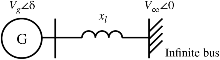
Figure 3.1 Single machine infinite bus system model.
The swing equation of a synchronous generator is given by
where ω is the angular velocity, M is the inertia constant, D is the damping coefficient, Pm is the mechanical input to the generator, Pe is the electrical output, Vg is the generator voltage, V∞ is the voltage of the infinite bus, δ is the rotor angle of the generator, x′d is the transient reactance of the generator, and xl is the line reactance. Note that the resistance of the generator and the transmission line is not considered for simplicity. In the swing equation (3.7), assuming that the voltages Vg and V∞ are constant, and ![]() ,
, ![]() , the deviation of the output power of the generator is given by
, the deviation of the output power of the generator is given by
where the subscript 0 is used to denote the initial value of the equilibrium point. Therefore, the swing equation (3.7) can be rewritten as
Here, the mechanical input Pm is assumed to be constant.
Finally, the linearized swing equation can be described by the following second-order linear differential equation:
The characteristic equation of the swing equation (3.10) is given by
The eigenvalue is the solution of the characteristic equation (3.11)
The time domain solution of the swing equation (3.10) is given by
where
If the real part of eigenvalues α is positive, the solution diverges, that is, the generator loses the synchronism. On the other hand, if the real part of eigenvalues α is negative, the solution converges to the equilibrium point, that is, the system maintains stability. Thus, the power system stability in the vicinity of the equilibrium point can be evaluated by calculating the eigenvalues of matrix A. In fact, the real part of eigenvalues provides an index for the degree of stability, and the imaginary part of the eigenvalues β corresponds to the angular velocity of oscillation.
3.2 Oscillation Model Identification Using Phasor Measurements
3.2.1 Oscillation Model of the Electromechanical Mode
The power swing equations of generators in an n-machine system can be represented by [7]
where i = 1, 2,…, n, ω is the angular velocity, δ is the rotor angle, M is the inertia constant, D is the damping coefficient, Pm is the mechanical input to the generator, Pe is the electrical output, and ωr is the rated angular velocity. When including the effect of other generator and controller dynamics, it is just assumed that their responses are sufficiently faster than the responses of the dominant modes. Interarea oscillations are mainly caused by the swing dynamics with a large inertia represented by (3.14). Now in this system suppose that the specific mode associated with power oscillation becomes unstable with the variation of a parameter such as changing the loading condition. The generator that significantly participates in the critical dominant oscillation mode can be easily identified by calculating the linear participation factor (2.6) [8].
As described in Chapter 2, interarea low-frequency oscillations involving both end generators are dominant in longitudinally interconnected power systems such as the western Japan 60 Hz power system. The characteristics of interarea oscillations caused by the inertia of some groups of synchronous generators could be represented by the same dynamics given by (3.14). Therefore, the interarea oscillation dynamics with a single mode can be simplified by assuming that it is analogous to a single machine and an infinite bus system:
Here, the dynamics of the critical dominant mode is represented by a simplified oscillation model. A second-order oscillation model can be identified in the following form by using time series data of voltage phasors of two measurement sites:

where ![]() and
and ![]() ; the subscript 1 denotes the selected site, the subscript s denotes the reference site, and subscript e denotes the initial phase angle. The coefficients a1 and a2 can be determined by the least squares method using acquired voltage phasor data. The characteristics of the dominant mode can be evaluated by the eigenvalues of the coefficient matrix A.
; the subscript 1 denotes the selected site, the subscript s denotes the reference site, and subscript e denotes the initial phase angle. The coefficients a1 and a2 can be determined by the least squares method using acquired voltage phasor data. The characteristics of the dominant mode can be evaluated by the eigenvalues of the coefficient matrix A.
Using steady-state phasor fluctuations, the model (3.16) can be identified. Hence, it is not necessary to stimulate the system by injecting a test signal such as an input step signal [9].
3.2.2 Dominant Mode Identification with Signal Filtering
Acquired voltage phasor data include many oscillation modes with different frequencies associated with interarea low-frequency oscillations with frequencies under 1 Hz, local modes with frequencies around 1 Hz, other modes with much lower frequencies associated with load frequency control issue. Therefore, the critical dominant mode should be extracted by some filtering techniques in order to estimate the simplified oscillation model (3.16) with higher accuracy. Here, two filtering methods are compared by focusing on the accuracy of the mode identification:
- Discrete wavelet transformation (DWT)-based filtering
- Fast Fourier transformation (FFT)-based filtering
The DWT can be used to decompose the signal into some signal components by keeping the time information. Therefore, the DWT can be an effective tool in detecting some events buried in the acquired time series data. The wavelet analysis decomposes a signal applying the shifting and scaling of the original (mother) wavelet. However, in the DWT, the passband of the signal decomposition filter is fixed since the filter is composed of a binary scale, that is, there is no flexibility to apply more detailed analysis [10].
Here, the application of the DWT to the power system oscillation data is considered. As described in Chapter 2, the interarea low-frequency oscillation mode is dominant in the whole system, and the characteristics of the mode can be identified by using the data acquired from both ends of the system since both end generators mainly participate in this mode. The oscillation mode between 0.2 and 0.8 Hz can be extracted by applying the DWT with the Symlet wavelet function.
On the other hand, the low-frequency mode might be extracted by acquired data from measurement units installed in the local area since the mode oscillates in the whole power system. It would be effective if the low-frequency mode could be detected by using only local measurements, for example, the measurements in the respective service areas since the data exchange between power companies might not be required in this case. However, the amplitude of the dominant oscillations included in the data measured in a local area should be smaller than the data measured in the wide area. That is, the influence of other modes becomes relatively larger; therefore, a specific filter with much narrower passband should be applied to extract the dominant mode and identify the dynamics with high accuracy.
Here, a band-pass filter based on the Fourier analysis with a sharp band-pass characteristic, while keeping the amplitude and the phase characteristics of the original data, is considered. Discrete Fourier transform and inverse transform for the finite number N of time series data x are given by
where W = exp(−j2p/N) and m, n = 0, 1,…, N −1. The procedure of filtering is to hold the Fourier transform X[m] of time series data x[n] corresponding to the frequencies of dominant modes and eliminate X[m] corresponding to the frequencies of other modes, then time series data of the dominant modes are reconstructed by the inverse transformation (3.18). It is noteworthy that this filter keeps the amplitude and phase of extracted oscillations. The following steps summarize the procedure of the stability assessment of the wide-area mode using the FFT-based filtering approach:
- Step 1: Analyze the Fourier spectrum of the phase differences.
- Step 2: Determine the center frequency fc of the band-pass filter by the spectrum in step 1.
- Step 3: Extract oscillation components from the original phase difference data using the FFT-based band-pass filter with fc ± 0.1 Hz.
- Step 4: Identify the simplified oscillation model (3.16) by using the extracted phase difference data, and then evaluate the eigenvalues of the dominant mode.
3.3 Small-Signal Stability Assessment of Wide-Area Power System
3.3.1 Simulation Study
Here, the described method for the small-signal stability assessment of the wide-area power system with phasor measurements is applied to a longitudinally interconnected six-machine power system shown in Fig. 3.2. The system constants are given in Table 2.1. Each generator is equipped with an automatic voltage regulator (AVR), which is shown in Fig. 2.2 [11]. The rated capacity of the generators is shown in Table 3.1.

Figure 3.2 Six-machine longitudinally interconnected power system model.
Table 3.1 Generator Rated Capacity (MVA)
| G1 | G2 | G3, G5 | G4 | G6 | Total Sum | |
| Case 1 | 20,000 | 13,500 | 6,750 | 40,000 | 33,000 | 120,000 |
| Case 2 | 16,000 | 10,800 | 5,400 | 32,000 | 27,000 | 96,600 |
| Case 3 | 12,000 | 8,000 | 4,000 | 24,000 | 20,000 | 72,000 |
Small load fluctuations measured in the steady-state operation can be used to identify (3.16), which represents the dynamics of the dominant mode. In this example, small load fluctuations are generated by slightly changing the load in order to simulate fluctuations measured in the real power system. Here, the stability assessment by the phasor measurements in the local area is considered. The simplified model (3.16) is identified by using the phase difference data between nodes 23 and 24 as adjacent measurement sites. The data length for the model identification is 200 s.
In case 1, the true eigenvalues of the dominant modes, calculated by the linearization of the system model, are −0.09 ± j1.93. When the DWT-based filter with the passband from 0.2 to 0.8 Hz is applied for extracting dominant oscillations, the coefficients of the identified model are a1 = −0.282 and a2 = −4.334, that is, the estimated eigenvalues are −0.14 ± j2.08. The result shows that the estimated eigenvalues are a little far from the real ones. On the other hand, when the FFT-based filter with the center frequency fc = 0.31 Hz and the passband between 0.19 and 0.43 Hz is applied, the coefficients of the identified model is a1 = −0.225 and a2 = −3.730, that is, the estimated eigenvalues are −0.11 ± j1.93. More close eigenvalues can be estimated by applying the FFT-based filtering. A narrower band-pass filter can be effective in eliminating the impact of other modes, especially in extracting the dominant oscillations from phase difference between adjacent measurement sites.
Figure 3.3 shows the original and filtered oscillations. Figure 3.3a shows the original second differentiation of the phase difference between nodes 23 and 24 before filtering. The dashed lines in Fig. 3.3b and c show the extracted second differentiation of the phase difference between nodes 23 and 24 by applying the DWT-based and the FFT-based filtering approaches, respectively. The solid lines show the waveform calculated by the identified model (3.16). Figure 3.3b shows that multiple modes are included in the waveform extracted by the DWT-based filtering since the amplitude of the dominant mode becomes comparable to other modes. On the other hand, Fig. 3.3c shows that a single mode is successfully extracted by specifying the passband of the FFT-based filtering method.

Figure 3.3 Original and filtered oscillations: (a) original, (b) DWT, and (c) FFT.
Table 3.2 summarizes the comparison of eigenvalues considering the type of filters for three cases. The value in the bracket indicates the residual for the least squares. Note that each value is normalized by each maximum value since the amplitude of the extracted waveform is different in each case. All results obtained from the FFT-based filtering have smaller error than the results given by the DWT-based filtering approach. These results demonstrate that the accuracy of the estimated eigenvalues can be improved by the FFT-based filtering method.
Table 3.2 Comparison of Eigenvalues with the Type of Filtering Method
| Original | DWT (Residual) | FFT (Residual) | |
| Case 1 | −0.09 ± j1.93 | −0.14 ± j2.08 (73.1) | −0.11 ± j1.93 (21.0) |
| Case 2 | −0.13 ± j2.85 | −0.17 ± j2.78 (46.2) | −0.12 ± j2.85 (26.5) |
| Case 3 | −0.16 ± j3.21 | −0.19 ± j3.07 (55.1) | −0.15 ± j3.22 (31.0) |
3.3.2 Stability Assessment Based on Phasor Measurements
The method is applied to phasor data measured in the real power system. Figure 3.4 shows the location of PMUs (Toshiba NCT2000) [12] installed at the western Japan 60 Hz power system. Figure 3.5 shows the Fourier spectrum of the phase difference data between Miyazaki and Nagoya (recorded at University of Miyazaki and Nagoya Institute of Technology-N.I.T., respectively), which are located at both ends of the system, and between Hiroshima and Osaka, which are located in the middle part of the system, respectively. The data of 200 s from 04:50 on July 1, 2006 are extracted by the DWT-based filter, which has the passband between 0.2 and 0.8 Hz. When using the phase difference between both ends, oscillations around 0.4 Hz, which are the interarea low-frequency mode, can be observed dominantly. On the other hand, when using the phase difference between adjacent sites, oscillations around 0.4 Hz can be observed; however, the amplitude becomes comparable to other modes.

Figure 3.4 The location of installed PMUs.
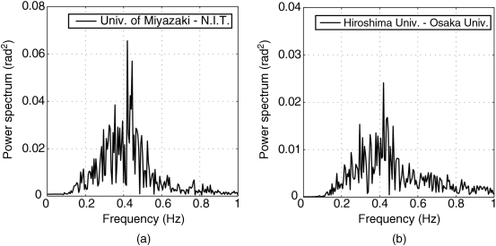
Figure 3.5 FFT results: (a) both ends and (b) middle.
Figure 3.6 shows the comparison of the accuracy of the simplified model (3.16) when the DWT- and the FFT-based filtering methods are applied to the phase difference between adjacent sites, respectively. The sum of square errors for DWT and FFT are 110.7 and 36.9, respectively, which are normalized by the maximum value. The accuracy of the identified model has been improved by the FFT-based filter.

Figure 3.6 Comparison of modeling accuracy: (a) DWT and (b) FFT.
Figure 3.7 shows the stability assessment of every hour for a week from July 1 to July 7 in 2006. Each eigenvalue is depicted by using 200 s data from 50 min of every hour. The reference of eigenvalues is the value estimated by using the phase difference between both ends.
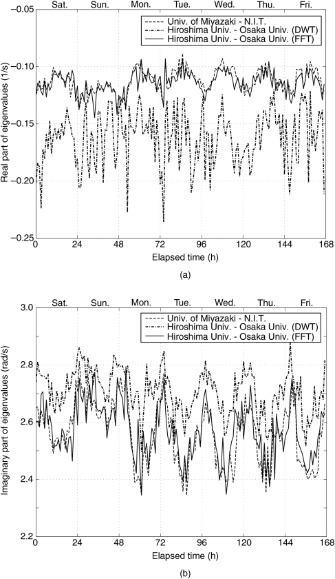
Figure 3.7 Comparison of eigenvalues: (a) real part and (b) imaginary part.
Figure 3.7 shows the comparison of the results of the two mentioned filters by using phase differences between adjacent sites. In the case of the DWT-based filtering, the estimated eigenvalues have larger errors with respect to the reference eigenvalues since the accuracy of the identified model deteriorates because the phase difference data includes multiple oscillation modes. On the other hand, in the case of FFT filtering, the daily change and the difference between weekdays and holidays of the stability of the low-frequency mode can be evaluated successfully since each eigenvalue has almost the same value as the reference. Thus, the wide-area stability can be evaluated with a high accuracy when using phasor data of the adjacent sites by improving the filter processing.
3.3.3 Stability Assessment Based on Frequency Monitoring
In a longitudinally interconnected power system, both end generators mainly participate in the low-frequency oscillation mode; therefore, the mode can be extracted from the phase difference between any two measurement sites in the system as described in the previous section. On the other hand, the mode can be extracted from the phasor information of just one measurement site located at one end since phasor oscillations of both ends have large amplitudes. Figure 3.8a shows the FFT spectrum for the phase difference between Miyazaki and Nagoya located at both ends of the system for data of 200 s from 13:50 on August 18, 2006. Figure 3.8b shows the FFT spectrum for the frequency deviations of Nagoya obtained by differentiating the measured phasors for the same period. The low-frequency oscillations with the frequency of about 0.4 Hz can be observed in both spectrums; however, Fig. 3.8b shows that the amplitude of this mode is comparable to other modes. Therefore, the DWT-based filter could not extract this mode properly since the influence of other modes could not be eliminated. Thus, the FFT-based filter should be applied here.

Figure 3.8 FFT spectrum for: (a) phase difference and (b) frequency deviation.
When using phasor data of two measurement sites, phasor oscillations can be observed clearly through calculating the phase difference of two sites by setting one site as the reference of the phase angle. However, when using measurement data of only one site, it is difficult to define the reference; therefore, the simplified model (3.16) cannot be applied to identify the low-frequency oscillations. Here, Fig. 3.9 shows the low-frequency oscillations extracted by the FFT-based filter using frequency deviation data measured at Miyazaki, Nagoya, and Tokushima, which are located at both ends and the middle part of the system, respectively. The low-frequency oscillations of Miyazaki and Nagoya change in opposite phases. On the other hand, the waveform of Tokushima has a smaller amplitude than the other two sites. This result implies that the fixed node of the low-frequency oscillation, that is ![]() , should exist near Tokushima. Thus, the oscillation model identified by using the information of only one measurement site can be considered by setting this point as the reference of the phase angle.
, should exist near Tokushima. Thus, the oscillation model identified by using the information of only one measurement site can be considered by setting this point as the reference of the phase angle.
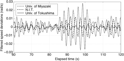
Figure 3.9 Filtered speed deviations of each point.
Assuming ![]() , the differentiation of the model (3.16) is
, the differentiation of the model (3.16) is
where ![]() and
and ![]() . The model (3.19) represents the oscillation dynamics of the low-frequency oscillation using the information of frequency deviations.
. The model (3.19) represents the oscillation dynamics of the low-frequency oscillation using the information of frequency deviations.
Figure 3.10 shows the result of a similar investigation as shown in Fig. 3.6. The sum of square errors for DWT and FFT are 110.4 and 69.0, respectively, where the amplitude is normalized by the maximum value. The accuracy of the identified model is improved by applying the FFT-based filtering method. Figure 3.11 shows the comparison results for the stability assessment for 1 week from August 13 to 19, 2006:
- The eigenvalues estimated by (3.16) identified using the phase difference between Miyazaki and Nagoya.
- The eigenvalues estimated by (3.19) identified using the frequency deviations of Nagoya.
- The eigenvalues estimated by (3.19) identified using the frequency deviations of Miyazaki.

Figure 3.10 Comparison of modeling accuracy: (a) DWT and (b) FFT.

Figure 3.11 Comparison of eigenvalues: (a) real part and (b) imaginary part.
The sum of square errors for Miyazaki–Nagoya, Nagoya, and Miyazaki are 32.0, 26.9, and 21.8, respectively. Therefore, the accuracy of the identified mode does not deteriorate even when using the frequency deviation data-based method. Since the eigenvalues can be estimated successfully, the frequency deviation data are effective in evaluating the stability of low-frequency oscillations.
3.4 Summary
This chapter describes the small-signal stability assessment with phasor measurements. Particularly, the stability of the interarea low-frequency oscillation mode has been investigated by adopting the method to identify the oscillation dynamics with a simple oscillation model. The filtering approach improves the accuracy of the estimated eigenvalues. The stability can be evaluated successfully by the presented approach.
References
- 1. J. A. Demcko, S. Pillutla, and A. Keyhani, Measurement of synchronous generator data from digital fault recorders for tracking of parameters and field degradation detection, Electr. Power Syst. Res., 39, 205–213, 1996.
- 2. C. Rehtanz and D. Westermann, Wide area measurement and control system for increasing transmission capacity in deregulated energy markets. In: Proceedings of the 14th Power Systems Computation Conference, 2002.
- 3. R. Avila-Rosales and J. Giri, Wide-area monitoring and control for power system grid security. In: Proceedings of the 15th Power Systems Computation Conference, 2005.
- 4. N. Kakimoto, M. Sugumi, T. Makino, and K. Tomiyama, Monitoring of interarea oscillation mode by synchronized phasor measurement, IEEE Trans. Power Syst., 21 (1), 260–268, 2006.
- 5. A. G. Phadke, Synchronized phasor measurements in power systems, IEEE Comput. Appl. Power, 6 (2), 10–15, 1993.
- 6. A. G. Phadke, et al., The wide world of wide-area measurement, IEEE Power Energy Mag., 6 (5), 52–65, 2008.
- 7. P. M. Anderson and A. A. Fouad, Power System Control and Stability, The Iowa State University Press, Ames, IA, 1977.
- 8. I. J. Peez-Arriaga, G. C. Verghese, and F. C. Schweppe, Selective modal analysis with application to electric power systems, part 1: heuristic introduction, IEEE Trans. Power Apparatus Syst., 101 (9), 3117–3125, 1982.
- 9. T. Hashiguchi, M. Watanabe, A. Matsushita, Y. Mitani, O. Saeki, K. Tsuji, M. Hojo, and H. Ukai, Identification of characterization factor for power system oscillation based on multiple synchronized phasor measurements, Electr. Eng. Jpn., 163 (3), 10–18, 2008.
- 10. The MathWorks, MATLAB Wavelet Toolbox. Wavelet Toolbox User's Guide, 2002.
- 11. Technical Committee of IEEJ, Japanese Power System Models, 1999. Available at http://www2.iee.or.jp/ver2/pes/23-st_model/english/index.html.
- 12. R. Tsukui, P. Beaumont, T. Tanaka, and K. Sekiguchi, Intranet-based protection and control, IEEE Comput. Appl. Power, 14 (2), 14–17, 2001.