
6
Wide-Area Measurement-Based Power System Control Design
Interconnections in a power system are intended to improve the system's reliability and economic efficiency. On the other hand, these interconnections occasionally cause interarea low-frequency oscillation with poor damping characteristics as described in Chapter 2. Therefore, many kinds of methods for designing a damping controller, such as a power system stabilizer (PSS), have been developed to damp interarea oscillations as well as local oscillations [1–3].
Recently, real-time monitoring of power systems based on the wide-area phasor measurement [4] has attracted the attention of power system engineers for the state estimation and system protection especially under a deregulated environment with complex power contracts. A proper grasp of the present state with flexible wide-area control should become a key issue in keeping power system stability properly. As mentioned in Chapter 2, the dynamic characteristics of oscillation modes, especially the interarea low-frequency mode with poor damping, can be detected successfully from phasor measurements [5]. Therefore, detected unstable modes can be damped adaptively and effectively by controlling the power system, for example, by tuning controller parameters based on the measurement data as described in Sections 4.1 and 5.2.
This chapter is mainly focused on the tuning of PSSs using wide-area phasor measurement. The identified low-order model based on the measurement represents power system oscillations, which can be used to design PSSs and to assess the effectiveness of PSS tuning in the real large-scale power system. Small-signal phasor fluctuations are available for the identification of the oscillation characteristics and the evaluation process for designed controllers. Therefore, damping controllers can be designed adaptively for a specific time interval. As a result, dominant swing modes are effectively damped by tuned controllers suitable for the present power system state. Some numerical analyses demonstrate the effectiveness of the method by using phasor dynamical data obtained by a power system simulation package.
6.1 Measurement-Based Controller Design
Many approaches for the measurement-based controller design have been investigated in the literatures such as the PSS design based on the Prony method [6], the identification of low-order state-space power system models by using multi-input multi-output procedures [7], and the low-order identification technique coupled with a robust controller design technique based on genetic algorithm [8]. These methods require some perturbation input to the system to identify the system state.
Figure 6.1 shows the schematic diagram of the concept of damping controller design based on the wide-area phasor measurements, which is described in this chapter. This diagram can be considered as an example realization scheme for the general real-time measurement-based approach described in Figs. 4.2 and 5.3. The advantage of the tuning scheme is that steady state phasor fluctuations are available for the identification process and the effect assessment of the tuned control. In other words, a large disturbance like a line fault is not necessary since the stability of dominant swing modes can be investigated directly by using eigenvalues of the identified model. Also, the identification process does not require information on the system input for perturbation, while the mentioned system identification methods require both input and output signals of the system.

Figure 6.1 Schematic diagram of damping controller design with wide-area measurements.
6.2 Controller Tuning Using a Vibration Model
6.2.1 A Vibration Model Including the Effect of Damping Controllers
The power swing equations of generators in an n-machine system can be represented by (3.14). In a multimachine power system multiple swing modes exist and interact with each other. For example, in a longitudinally interconnected power system like the western Japan 60 Hz system, two interarea modes associated with power oscillations tend to be dominant and interact with each other [9]. One of the modes is associated with the oscillation between both end generators; the other is associated with the oscillation among three generators, which are both ends and the middle one. These oscillation characteristics can be explained by right eigenvectors (2.4) and the participation factor (2.6). Note that the following method is applicable to any other system such as a longitudinal system in cases where characteristic oscillations are observed.
Here, a coupled vibration model is considered to represent the interaction of two modes. These modes are assumed to oscillate with keeping the dynamics of power swing equations (3.14). The first vibration model corresponds to the most dominant mode, while the other corresponds to the second dominant mode. Three observation sites near generators that significantly participate in these two modes are selected; then, one end site is used as the reference of the phase angle. The dynamics of the model is represented by the polynomial approximation of the phase angle and the angular velocity:
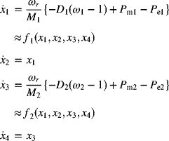
Here, functions f1 and f2 are assumed to consist of linear terms

where ![]() ,
, ![]() ,
, ![]() and
and ![]() . Subscripts 1 and 2 denote numbers of selected sites, the subscript “s” denotes the reference site, and the subscript “e” denotes the initial value of the phase angle at t = 0. The coefficients ai and bi (i = 1 ∼ 4) can be evaluated by applying the least squares method to time series data sets of xj (j = 1 ∼ 4) obtained by the wide area phasor measurement. Oscillation characteristics are investigated directly by using this model since eigenvalues of the coefficient matrix represent the damping and frequency of two oscillatory modes. If necessary, this model can be extended to the case expressed in more than two dominant modes, that is, by increasing state variables and choosing the corresponding measurement sites according to the number of the dominant modes.
. Subscripts 1 and 2 denote numbers of selected sites, the subscript “s” denotes the reference site, and the subscript “e” denotes the initial value of the phase angle at t = 0. The coefficients ai and bi (i = 1 ∼ 4) can be evaluated by applying the least squares method to time series data sets of xj (j = 1 ∼ 4) obtained by the wide area phasor measurement. Oscillation characteristics are investigated directly by using this model since eigenvalues of the coefficient matrix represent the damping and frequency of two oscillatory modes. If necessary, this model can be extended to the case expressed in more than two dominant modes, that is, by increasing state variables and choosing the corresponding measurement sites according to the number of the dominant modes.
On the other hand, the oscillation data obtained by the wide area measurement are the phase angle and include many frequency components associated with interarea low-frequency oscillations as well as local oscillations and many noises. Here, discrete wavelet analysis is applied to extract oscillations including the dominant two modes from measurement data. Interarea oscillations with frequencies between 0.2 and 0.8 Hz can be extracted, while modes with frequencies smaller than 0.2 Hz including DC components, local modes with frequencies higher than 1.0 Hz, and many noises with high frequencies can be eliminated by using wavelet transformation. Thus, data sets of phase difference x2 and x4 are provided. On the other hand, the angular velocity x1 and x3 can be calculated by differentiating x2 and x4, respectively.
Identified interarea low-frequency modes by using the mentioned method have occasionally poor damping characteristics. These modes, which are dominant in the wide-area stability, might become unstable with a heavier load on the tie-lines. Therefore, these modes must be damped by controlling the power system. The use of PSS is effective to stabilize interarea modes. Here, an approach for tuning of PSSs based on the phasor measurement is described.
Assume a dynamic model of the k-th PSS (with similar structure shown in Fig. 5.2) as follows,
which describes the typical real one consisting of a two-stage lead-lag compensation. Here, T1k, …, T4k are time constants, Kk is a gain, T0 is time lag for the signal detection, and Tw is the time constant of the signal washout. In this study, PSS, which feeds back the generator angular velocity deviation Δω, is assumed, since a Δω-type PSS is more effective to damp interarea oscillations. When feeding back the generator output deviation ΔP, which is effective to damp local modes with frequency around 1.0 Hz, there is a necessity to carry out a synchronized measurement of the ΔP, or identify the ΔP from the measured phasors.
Here, the coupled vibration model (6.2) is extended for including the effect of PSSs:

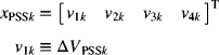
where xPSSk (k = 1, 2) is the vector of state variables of PSS defined by
where the superscript “T” stands for the transposition of vector. Variables x2 and x4 are directly measured by the PMUs. Other ones can be calculated by the relations of ![]() ,
, ![]() , and (6.3) from the measured x2 and x4.
, and (6.3) from the measured x2 and x4.
The vectors ck (k = 1, 2), which are calculated simultaneously with ![]() and
and ![]() (i = 1 ∼ 4) by the least squares method, imply the effect of PSS on each oscillation mode. Note that only one of the elements of ck associated with the PSS output (v1k) has any value, while all other elements are equal to zero, that is,
(i = 1 ∼ 4) by the least squares method, imply the effect of PSS on each oscillation mode. Note that only one of the elements of ck associated with the PSS output (v1k) has any value, while all other elements are equal to zero, that is,

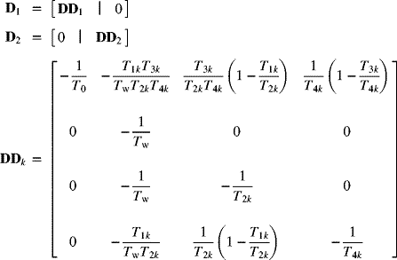
The 4 × 1 vector dk and the 4 × 8 matrix Dk are determined by the real structure of object PSS (6.3), which contains the parameters Kk, T0, Tw, and T1k,…, T4k.
Note that the input of each PSS in the model (6.4) is ![]() and
and ![]() , respectively, although it is different from the real input signal of the Δω-type PSS. The model (6.4) should be considered to be a simplified model specialized for tuning of PSSs to search the appropriate direction of tuning parameters. The stability of dominant modes is evaluated by eigenvalues of matrix (6.4).
, respectively, although it is different from the real input signal of the Δω-type PSS. The model (6.4) should be considered to be a simplified model specialized for tuning of PSSs to search the appropriate direction of tuning parameters. The stability of dominant modes is evaluated by eigenvalues of matrix (6.4).
6.2.2 Tuning Mechanism
Two PSSs are tuned based on the model (6.4) since vectors dk and matrices Dk include parameters of PSSs, and the change of parameters affect eigenvalues directly. Tuned parameter sets are expected to stabilize at least two modes although they could not be optimum sets. The effectiveness of the tuning approach can be assessed more properly by evaluating the eigenvalues of (6.4), which is obtained from measurement data after applying the tuned control method. Thus, the PSS parameters can be tuned based on the small-signal oscillation data obtained by the wide-area phasor measurement.
The obtained new PSS parameter sets by the mentioned approach are the final goal of the proposed tuning method. However, the obtained parameter sets might be affected by an error in the calculation process, a large noise in the measurement data, a sudden change of the system state, and the adverse effect on other modes that are not considered in the model (6.4). Therefore, the PSSs must be tuned by gradual steps for the security of the power system. This gradual tuning mechanism is also applicable in the case of using other methods for tuning of PSS parameters, such as identification-based methods, genetic algorithm, fuzzy logic, and so on.
The wide-area phasor measurement-based PSS tuning mechanism using the described extended coupled vibration model (6.4) consists of the following steps:
- Step 1: Select three measurement sites, which significantly participate in the dominant and the quasi-dominant modes. One of them is for the reference of the phase angle and the other two are targets of the tuning issue.
- Step 2: Obtain the oscillation data from the sites. Steady state phasor fluctuations measured in the normal operation are available. Note that phasors with time labels are stored using the installed PMUs (synchronized by the GPS signal). Therefore, measured phasors are directly comparable with each other without considering the communication delay.
- Step 3: Extract interarea oscillations by applying the discrete wavelet transformation to the observed phasor. The time series data sets of the PSS state variables can be provided by calculating (6.3) in the time domain.
- Step 4: Determine coefficients
 ,
,  , and ck of the coupled vibration model (6.4) by the least squares method.
 - Step 5: Find appropriate parameter sets of PSSs based on the model (6.4).
- Step 6: Tune the PSSs step by step toward the parameter sets obtained in the previous step. In each step, the effect of tuning is assessed by eigenvalues of (6.4) that is modeled again using the phasor fluctuations after tuning control.
- Step 7: By repeating the gradual tuning and the stability assessment, the PSSs can be tuned appropriately.
Here, a coupled vibration model with two dominant electro-mechanical modes associated with the angle stability is discussed. Therefore, this approach is applicable in the case that a dominant and a quasi-dominant mode are classified while the participating measurement sites (in these modes) are specified. Note that the application of this approach is not limited to the power system with longitudinal configuration used in this study.
6.2.3 Simulation Results
The method is applied to a 10-machine longitudinally interconnected system. Figure 6.2 shows the configuration of the IEEJ WEST 10-machine system model. The detailed parameters and relevant data are available in Ref. [10]. This test system represents the power system model of the western 60 Hz areas of Japan. System constants and generation capacity of generators are shown in Tables 2.1 and 6.1, respectively. The active power of all loads is assumed to have constant current characteristics, and reactive power is considered with constant impedance characteristics. In Fig. 6.2, (P) denotes the generation and loading condition in the daytime and (N) denotes the condition in the nighttime. The unit is 1000 MVA base per unit.
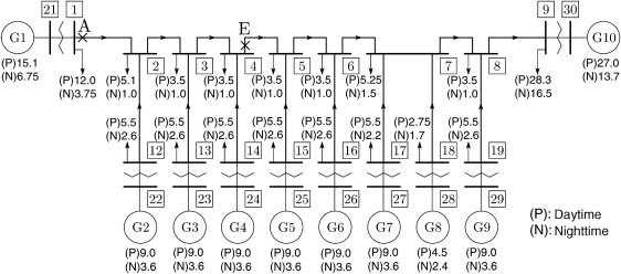
Figure 6.2 IEEJ WEST 10-machine system model.
Table 6.1 Generator Rated Capacity (MVA)
| Daytime, MVA | Nighttime, MVA | |
| G1 | 15,000 | 9,000 |
| G8 | 5,000 | 3,000 |
| G10 | 30,000 | 18,000 |
| Others | 10,000 | 6,000 |
| Total sum | 120,000 | 72,000 |
Each generator is equipped with an automatic voltage regulator (AVR) shown in Fig. 6.3, and generators 1 and 5 are equipped with the Δω-type PSS to damp the interarea oscillations. In this study, the time lag for the signal detection and the time constant of the signal washout are T0 = 0.02 (s), Tw = 5.0 (s), respectively. In the initial/nominal condition, the parameter setting of PSS is K = 0.20, T1 = 1.66, T2 = 1.51, T3 = 2.07, T4 = 0.01, and two generators are equipped with the identical PSS. In this study, the EUROSTAG software [11] is used for the time domain simulation of the power system dynamics.

Figure 6.3 Exciter model with the Δω type PSS.
Figure 2.3 shows the real part of the right eigenvectors corresponding to the generator rotor angle in the daytime loading condition. Mode 1 denotes the dominant mode, and mode 2 denotes the quasi-dominant mode. This result shows that mode 1 oscillates in the opposite direction between both end generators 1 and 10, while mode 2 oscillates between both end generators 1, 10, and the middle generator 5. Figure 2.4 shows participation factors corresponding to the generator rotor angle. These results show that generators 1, 5, and 10 participate principally in modes 1 and 2. Here, the coupled vibration model is calculated by using the voltage phasor of nodes 21 and 25 with node 30 as a reference.

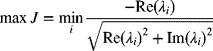
Figure 6.4 Simulation with the tuned PSSs of generators 1 and 5 in the daytime condition. (a) Generator 1. (b) Generator 5.
In this study, some small load variations at some load buses are assumed to simulate the phasor fluctuations measured in the real power system. The extended coupled vibration model (6.4) is constructed by using these small oscillations. Table 6.2 shows the eigenvalues variation when each parameter of the connected PSS to the generator 1 is changed. The second column of the table shows eigenvalues of dominant low-frequency modes calculated by using the power system simulation package. The third column shows eigenvalues of the corresponding two modes of the approximate model (6.4). The result shows that the approximate model estimates two conjugate eigenvalues, properly. In addition, the trend of the variation of both eigenvalues with parameter change coincides well with each other. Therefore, the extended coupled vibration model can correctly evaluate the stability change with tuning of PSS parameters. The advantage of this approach is in estimating the dominant modes by using steady state phasor fluctuations measured in the normal operating condition.
Table 6.2 The Comparison of Eigenvalues Variation of the Original System and the Approximate Model, When the Parameters of the Connected PSS to Generator 1 are Changed in the Daytime Loading Condition
| Parameters | Full System | Approximate Model |
| Initial condition | −0.065 ± j1.731 −0.154 ± j4.055 |
−0.080 ± j2.223 −0.182 ± j3.832 |
| K = 0.02 | −0.048 ± j1.714 −0.152 ± j4.050 |
−0.074 ± j2.152 −0.179 ± j3.815 |
| K = 0.4 | −0.080 ± j1.751 −0.157 ± j4.061 |
−0.085 ± j2.292 −0.184 ± j3.847 |
| T1 = 2.16 | −0.071 ± j1.735 −0.155 ± j4.057 |
−0.082 ± j2.248 −0.183 ± j3.835 |
| T1 = 1.16 | −0.058 ± j1.728 −0.153 ± j4.054 |
−0.078 ± j2.196 −0.181 ± j3.828 |
| T2 = 2.01 | −0.059 ± j1.728 −0.154 ± j4.054 |
−0.078 ± j2.201 −0.181 ± j3.828 |
| T2 = 1.01 | −0.076 ± j1.736 −0.156 ± j4.058 |
−0.083 ± j2.261 −0.183 ± j3.836 |
| T3 = 2.57 | −0.070 ± j1.735 −0.155 ± j4.057 |
−0.082 ± j2.243 −0.183 ± j3.835 |
| T3 = 1.57 | −0.060 ± j1.728 −0.154 ± j4.054 |
−0.078 ± j2.202 −0.181 ± j3.828 |
| T4 = 0.51 | −0.048 ± j1.732 −0.150 ± j4.052 |
−0.075 ± j2.154 −0.179 ± j3.826 |
Table 6.3 shows the result of tuning of PSSs based on the approximate model (6.4). The PSS parameter sets are determined to improve damping ratios of two low-frequency modes of the model, that is, to maximize the following objective function J under the constraint that all eigenvalues lie on the left-hand side of the complex plane:
subject to
where λi is the i-th eigenvalue of the model (6.4). The ![]() and
and ![]() denotes the real and imaginary parts of the i-th eigenvalue, respectively. The optimization is implemented by using the MATLAB® Toolbox for genetic algorithm [12].
denotes the real and imaginary parts of the i-th eigenvalue, respectively. The optimization is implemented by using the MATLAB® Toolbox for genetic algorithm [12].
Table 6.3 Result of the PSS Tuning in the Daytime Condition
| Parameter | Initial | G1 | G5 |
| K | 0.20 | 0.37 | 0.23 |
| T1 | 1.66 | 1.82 | 2.64 |
| T2 | 1.51 | 0.83 | 0.64 |
| T3 | 2.07 | 2.31 | 2.09 |
| T4 | 0.01 | 0.01 | 0.01 |
Table 6.4 shows parameter settings for five steps of gradual tuning of the PSS connected to generator 1. One wrong case with the opposite direction of parameter tuning is also considered for investigating the accuracy of the proposed method. Table 6.4 also shows eigenvalues of the coupled vibration model (6.4) and damping ratios in each parameter setting. The result shows that two dominant modes are stabilized gradually with the parameter change from the initial parameter set to the final set. On the other hand, in the wrong case, two modes are destabilized with the change of parameters. In case of considering the connected PSS to generator 5, similar results have been obtained. These results show that appropriate parameters of PSSs can be obtained and the stability change can be exactly assessed by using the coupled vibration model.
Table 6.4 The Stability Change with Gradual Tuning of PSS Connected to Generator 1
| Parameter Sets | K | T1 | T2 | T3 | T4 | Eigenvalues of the Approximate Model | Damping Ratio, % |
| Wrong | 0.16 | 1.63 | 1.66 | 2.02 | 0.01 | −0.0781 ± j2.1976 −0.1808 ± j3.8266 |
3.554 4.720 |
| Initial | 0.20 | 1.66 | 1.51 | 2.07 | 0.01 | −0.0801 ± j2.2230 −0.1816 ± j3.8316 |
3.601 4.735 |
| First | 0.24 | 1.69 | 1.36 | 2.12 | 0.01 | −0.0822 ± j2.2521 −0.1828 ± j3.8369 |
3.646 4.759 |
| Second | 0.28 | 1.72 | 1.21 | 2.17 | 0.01 | −0.0845 ± j2.2868 −0.1841 ± j3.8426 |
3.691 4.786 |
| Third | 0.32 | 1.75 | 1.06 | 2.22 | 0.01 | −0.0866 ± j2.3250 −0.1854 ± j3.8478 |
3.723 4.812 |
| Fourth | 0.36 | 1.78 | 0.91 | 2.27 | 0.01 | −0.0886 ± j2.3644 −0.1868 ± j3.8522 |
3.744 4.843 |
| Final | 0.37 | 1.82 | 0.83 | 2.31 | 0.01 | −0.0894 ± j2.3836 −0.1876 ± j3.8531 |
3.749 4.862 |
Figure 6.4 shows the simulation results when two tuned PSSs are applied, simultaneously. Here, a three-phase ground fault at point E in the double circuit transmission line, which is shown in Fig. 6.2, is assumed as a disturbance. The fault is cleared at 0.07 s after the fault occurred. The result shows that low-frequency oscillation is effectively damped by the tuned PSSs. On the other hand, the critical clearing time, which was 0.091 s in the initial condition, is improved up to 0.142 s with the tuned PSSs.
The proposed method is applied to a different loading condition. The loading condition denoted by (N) in Fig. 6.2 is used in this analysis. Table 6.5 shows the comparison of eigenvalues calculated by using the full system matrix with the approximate coupled vibration model. The result shows that the approximate model successfully evaluates the slight change of eigenvalues.
Table 6.5 The Comparison of Eigenvalues Variation of the Original System and the Approximate Model, When the Parameters of the Connected PSS to Generator 1 is Changed in the Nighttime Loading Condition
| Parameters | Full System | Approximate Model |
| Initial condition | −0.1021 ± j2.7001 −0.1912 ± j5.0542 |
−0.0875 ± j2.7733 −0.2346 ± j4.3954 |
| K = 0.02 | −0.0996 ± j2.6966 −0.1902 ± j5.0497 |
−0.0872 ± j2.7699 −0.2341 ± j4.3900 |
| K = 0.4 | −0.1049 ± j2.7040 −0.1924 ± j5.0591 |
−0.0878 ± j2.7771 −0.2358 ± j4.4002 |
| T1 = 2.16 | −0.1032 ± j2.7011 −0.1918 ± j5.0557 |
−0.0878 ± j2.7747 −0.2352 ± j4.3969 |
| T1 = 1.16 | −0.1010 ± j2.6992 −0.1907 ± j5.0527 |
−0.0870 ± j2.7716 −0.2344 ± j4.3930 |
| T2 = 2.01 | −0.1013 ± j2.6993 −0.1908 ± j5.0530 |
−0.0873 ± j2.7724 −0.2347 ± j4.3929 |
| T2 = 1.01 | −0.1040 ± j2.7014 −0.1923 ± j5.0565 |
−0.0888 ± j2.7765 −0.2354 ± j4.3979 |
| T3 = 2.57 | −0.1029 ± j2.7010 −0.1916 ± j5.0554 |
−0.0876 ± j2.7744 −0.2351 ± j4.3965 |
| T3 = 1.57 | −0.1013 ± j2.6993 −0.1908 ± j5.0530 |
−0.0873 ± j2.7725 −0.2347 ± j4.3931 |
| T4 = 0.51 | −0.0984 ± j2.6990 −0.1885 ± j5.0503 |
−0.0651 ± j2.7355 −0.2300 ± j4.3518 |
Table 6.6 and Fig. 6.5 show the results of tuning the PSSs. Assumed disturbance is the same fault at point A in Fig. 6.2, where it is cleared at 0.07 s after the fault occurred. The critical clearing time is improved from 0.070 s up to 0.087 s. These results demonstrate the effectiveness of the proposed approach based on the wide-area phasor measurement.
Table 6.6 The Result of PSSs Tuning in the Nighttime Condition
| Parameters | Initial | G1 | G5 |
| K | 0.20 | 0.31 | 0.67 |
| T1 | 1.66 | 4.52 | 1.91 |
| T2 | 1.51 | 0.68 | 0.43 |
| T3 | 2.07 | 3.58 | 2.98 |
| T4 | 0.01 | 0.01 | 0.01 |
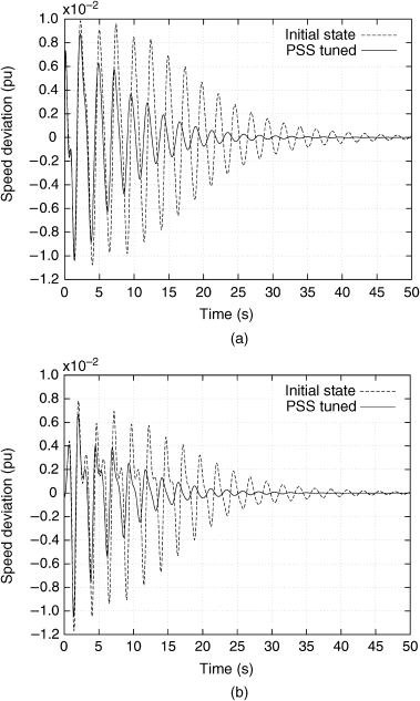
Figure 6.5 Simulation with the tuned PSSs of generators 1 and 5 in the nighttime condition. (a) Generator 1. (b) Generator 5.
6.3 Wide-Area Measurement-Based Controller Design
6.3.1 Wide-Area Power System Identification
This section introduces another approach for tuning of the damping controller with wide-area phasor measurements. The interarea oscillation dynamics with a single mode can be simplified by assuming that it has an analogy of a single machine and infinite bus system:
Using voltage phasors of two measurement sites, a second-order oscillation model for the dominant oscillation mode can be identified in the following form:
where ![]() , and
, and ![]() . The subscript 1 denotes the selected site, the subscript “s” denotes the reference site, and subscript “e” denotes the initial phase angle at t = 0. The coefficients a1 and a2 can be determined by the least squares method by using filtered voltage phasors data with the fast Fourier transform (FFT)-based filtering method described in Chapter 2. The characteristics of the extracted mode can be evaluated by the eigenvalues of the coefficient matrix A. Assuming that the eigenvalues are given by α ± jβ, the approximate oscillation model of the interested mode is represented by the following form:
. The subscript 1 denotes the selected site, the subscript “s” denotes the reference site, and subscript “e” denotes the initial phase angle at t = 0. The coefficients a1 and a2 can be determined by the least squares method by using filtered voltage phasors data with the fast Fourier transform (FFT)-based filtering method described in Chapter 2. The characteristics of the extracted mode can be evaluated by the eigenvalues of the coefficient matrix A. Assuming that the eigenvalues are given by α ± jβ, the approximate oscillation model of the interested mode is represented by the following form:
Considering a damping controller design, the control loop with the oscillation model G(s) and a controller is assumed as shown in Fig. 6.6. Here, the damping controller, where a PSS is considered in this study, includes the real structure of the controller, and the model F(s) represents the effect of the controller on the oscillation mode G(s). In order to simplify the procedure of the controller design, the order of F(s) should be reduced as much as possible. In this study, the model F(s) is assumed by the following form:

Figure 6.6 Approximate low-order model for tuning the Δω-type PSS to damp inter-area low-frequency oscillation.
The procedure of determining the model F(s) is as follows:
- Step 1: Determine time constants Ta ∼ Td to maximize the gain characteristics around the frequency, which corresponds to the imaginary part of the estimated eigenvalue (β).
- Step 2: Set the time constant Te at about zero degree of the frequency response of F(s) around the frequency, which corresponds to the imaginary part β of the estimated eigenvalue.
- Step 3: Compute the gain K to minimize the mean square error between the filtered phase difference and the output of the approximate model shown in Fig. 6.6.
6.3.2 Design Procedure
Here, the H∞ control theory is applied to the approximate low-order system model shown in Fig. 6.6 to compensate for the modeling error. Figure 6.7 shows the generalized plant including two weighting functions, Ws(s) and Wt(s). The Ws(s) has low-pass filter characteristics to consider the robust stability and modeling error, while Wt(s) has high-pass filter characteristics to consider the influence of other modes. The H∞ norm of the closed-loop system can be given by
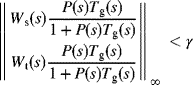
where P(s) is the transfer function of the controller. Tg(s) is the transfer function of the generalized plant including the simplified model G(s), F(s), and scaling factor. An H∞ controller satisfying (6.15) is designed for the minimum γ, as the H∞ robustness index.
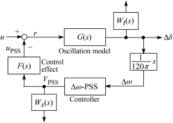
Figure 6.7 Closed-loop system configuration.
Note that the designed controller generally has a high order; therefore, the order of the controller should be as low as possible to simplify the tuning process. In this study, the balanced realization technique is adopted to obtain a low-order controller from the original designed H∞ controller. It is noteworthy that instead of H∞ control, other robust/advanced control techniques such as H2 and μ control synthesis methods can be also used [13].
6.3.3 Simulation Results
The method is applied to the simple 11-bus two-area power system model shown in Fig. 6.8. System constants including detailed bus and line data as well as the generators and load parameters are given in Ref. [14].

Figure 6.8 Simple two-area system model.
Generator 1 is equipped with an AVR and a Δω-type PSS shown in Fig. 6.9 to damp interarea oscillations. PSS parameters for the initial condition are KSTAB = 5.0, T1 = 2.0, T2 = 1.0, T3 = 2.0, and T4 = 0.5. Here, KSTAB is the PSS gain. Other generators are equipped with the identical AVR with PSS shown in Fig. 6.10. The effect of the speed governor is not considered. In this study, the EUROSTAG software [11] has been used for the simulation of the power system dynamics.
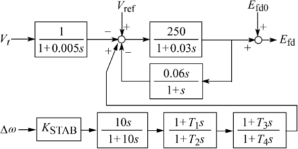
Figure 6.9 Exciter and PSS model for generator 1.

Figure 6.10 Exciter and PSS model for generators 2, 3, and 4.
First, the system is examined without connecting the PSS of generator 1. The small load fluctuations at node 7 are assumed to simulate the phasor fluctuations measured in the normal condition of the real power system. Figure 6.11 shows the phase differences between nodes 1 and 3. Figure 6.12 shows the Fourier spectrum of Fig. 6.11. The result shows that an interarea oscillation mode with frequency of around 0.60 Hz is dominant.
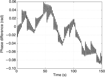
Figure 6.11 Phase difference between nodes 1 and 3.
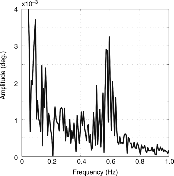
Figure 6.12 Fourier spectrum.
Figure 6.13 shows the phase difference of interarea low-frequency oscillations extracted by the FFT-based filter, where the frequency band width is set to 0.60 ± 0.04 Hz. A simplified oscillation model (6.12) is identified by applying the least squares method to the filtered phase difference data. The eigenvalues of the coefficient matrix A are α ± jβ = −0.137 ± j3.720. Substituting the obtained values into (6.12), the oscillation model (6.13) is represented as follows:

Figure 6.13 Filtered phase difference.
The model F(s) is identified by using the procedure described in Section 6.3.1. The model F(s) is given by
Figure 6.14 illustrates the bode diagram of the model F(s), which has the gain peak at 3.77 rad/s.

Figure 6.14 Bode diagram of the model F(s).
The input u of the approximate model shown in Fig. 6.6 is estimated by multiplying the inverse function of (6.16) to filtered phase difference data. Figure 6.15 shows the estimated input signal u of the approximate model. Figure 6.16 shows the comparison between the filtered phase difference of measured data and the approximate model output simulated by using the estimated input signal. These results demonstrate that the approximate model can successfully represent the characteristics of the interarea low-frequency oscillation mode and the effect of the controller on this mode.
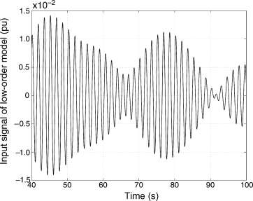
Figure 6.15 The input signal u for the low-order model.
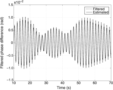
Figure 6.16 The comparison between the filtered phase difference and the output signal of the low-order model.
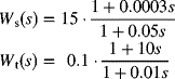
The H∞ controller is designed for the identified low-order system model. The controller corresponding to the minimum γ satisfying the constraint (6.15) is derived based on the generalized plant shown in Fig. 6.7. Two weighting functions Ws(s) and Wt(s) are given by
The H∞ controller is derived in the following form:
The coefficients of the H∞ controller (6.19) are shown in Table 6.7.
Table 6.7 The Coefficients of H∞ Controller
| a7 | 1.39 × 10⁶ | b7 | 3161 |
| a6 | 1.64 × 10⁸ | b6 | 4.88 × 10⁵ |
| a5 | 4.03 × 10⁹ | b5 | 2.02 × 10⁷ |
| a4 | 3.03 × 10¹⁰ | b4 | 1.85 × 10⁸ |
| a3 | 8.94 × 10¹⁰ | b3 | 5.93 × 10⁸ |
| a2 | 9.46 × 10¹⁰ | b2 | 7.10 × 10⁸ |
| a1 | 1.20 × 10¹⁰ | b1 | 2.06 × 10⁷ |
| a0 | 3.43 × 10⁸ | b0 | 1.40 × 10⁷ |
By applying the balanced realization technique to the H∞ controller (6.19), the final model of reduced order PSS is obtained as follows:
Figure 6.17 demonstrates a comparison of bode diagrams of the H∞ controller (6.19) and the designed PSS (6.20). The result shows that the designed PSS (6.20) with third order is the same in performance with the H∞ controller (6.19) with eighth order.
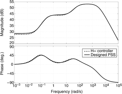
Figure 6.17 The comparison of bode diagrams between the full-order (6.19) and the reduced-order (6.20) H∞ controllers.
Here, the performance of the designed PSS (6.20) by the proposed method is evaluated. Table 6.8 shows eigenvalues of the interarea low-frequency mode and two local modes of the original system model shown in Fig. 6.8. Appropriate parameters of the PSS can be obtained since the interarea mode is damped effectively. Note that the low-order model does not consider other modes than the interarea mode; therefore, it is difficult to evaluate the influence of the parameter tuning of the controller on other modes on the low-order model. In this case, the influence is not so large as shown in Table 6.8 since local modes have larger damping than the interarea mode.
Table 6.8 The Eigenvalues of the Simple Two-Area System
| Mode | Interarea | Area 1 Local | Area 2 Local |
| Without PSS | −0.123 ± j3.710 | −0.958 ± j6.863 | −1.176 ± j7.763 |
| Initial PSS | −0.201 ± j3.814 | −0.916 ± j7.243 | −1.175 ± j7.764 |
| Designed PSS | −0.322 ± j4.071 | −0.830 ± j8.743 | −1.173 ± j7.760 |
Figure 6.18 shows the step response of the approximate model, where the magnitude of the step input has been adjusted to be consistent with the response of the original system shown in Fig. 6.19. The result shows that the designed PSS (6.20) can damp the low-frequency oscillation more effectively than the initial condition.

Figure 6.18 Step response with the low-order model.

Figure 6.19 Simulation result with the original two-area system.
On the other hand, Fig. 6.19 shows the simulation results of the original system shown in Fig. 6.8. An assumed disturbance here is a three-phase to ground fault between nodes 7 and 8. The fault is cleared at 0.067 s after the fault. The result shows that the interarea oscillation is effectively damped by the designed PSS.
Comparing Fig. 6.18 with Fig. 6.19, characteristics of the interarea low-frequency oscillation of the original system can be represented approximately by the low-order model. These results demonstrate the effectiveness of the proposed method based on wide-area phasor measurements considering the error compensation with H∞ control theory.
6.4 Summary
This chapter describes a method for tuning of PSSs based on wide-area phasor measurements. The low-order system model, which holds the characteristics of the interarea oscillation mode and the control effect, is identified by monitoring data from wide-area phasor measurements. The effectiveness of the proposed method has been demonstrated through the power system simulation. The results show that an appropriate controller can be designed by using the identified low-order model.
References
- 1. T. Michigami, Development of a new two-input PSS to control low-frequency oscillation in interconnecting power systems and the study of a low-frequency oscillation model, Electr. Eng. Jpn., 115 (7), 49–68, 1995.
- 2. T. Senjyu, T. Yamashita, and K. Uezato, Stabilization control of multi-machine power systems by adaptive power system stabilizer using frequency domain analysis, Electr. Eng. Jpn., 142(2), 10–20, 2003.
- 3. M. Ishimaru, R. Yokoyama, O. M. Neto, and K. Y. Lee, Allocation and design of power system stabilizers for mitigating low-frequency oscillations in the eastern interconnected power system in Japan, Int. J. Electr. Power Energy Syst., 26 (8), 607–618, 2004.
- 4. A. G. Phadke, Synchronized phasor measurements in power systems, IEEE Comput. Appl. Power, 6 (2), 10–15,1993.
- 5. T. Hashiguchi, M. Watanabe, A. Matsushita, Y. Mitani, O. Saeki, K. Tsuji, M. Hojo, and H. Ukai, Identification of characterization factor for power system oscillation based on multiple synchronized phasor measurements, Electr. Eng. Jpn., 163 (3), 10–18, 2008.
- 6. D. J. Trudnowski, J. R. Smith, T. A. Short, and D. A. Pierre, An application of Prony methods in PSS design for multimachine systems, IEEE Trans. Power Syst., 6 (1), 118–126, 1991.
- 7. I. Kamwa, G. Trudel, and L. Gerin-Lajoie, Low-order black-box models for control system design in large power systems, IEEE Trans. Power Syst., 11 (1), 303–311, 1996.
- 8. A. Hasanovic, A. Feliachi, A. Hasanovic, N. B. Bhatt, and A. G. DeGroff, Practical robust PSS design through identification of low-order transfer functions, IEEE Trans. Power Syst., 19 (3), 1492–1500, 2004.
- 9. N. Kakimoto, A. Nakanishi, and K. Tomiyama, Instability of interarea oscillation mode by autoparametric resonance, IEEE Trans. Power Syst., 19 (4), 1961–1970, 2004.
- 10. Technical Committee of IEEJ, Japanese Power System Models, 1999. Available at http://www2.iee.or.jp/ver2/pes/23-st_model/english/index.html.
- 11. M. Stubbe, A. Bihain, J. Deuse, and J. C. Baader, STAG: a new unified software program for the study of the dynamic behaviour of electrical power systems, IEEE Trans. Power Syst., 4 (1), 129–138, 1989.
- 12. GAOT: A Genetic Algorithm for Function Optimization: A Matlab Implementation, 1995. Available at http://www.ie.ncsu.edu/mirage/GAToolBox/gaot/.
- 13. H. Bevrani, Robust Power System Frequency Control, Springer, New York, 2009.
- 14. P. Kundur, Power System Stability and Control, McGraw-Hill, New York, 1994.