
10
Microgrid Control: Synthesis Examples
In Chapter 9, the concept of the microgrid (MG) was explained. The MG control loops are divided into four control levels: primary, secondary, global, and central/emergency controls. In this chapter, some design examples for these control levels are briefly discussed. Interested readers can find more details in the authors' previous publications [1–18].
10.1 Local Control Synthesis
10.1.1 Robust Voltage Control Design [4]
As an example for local control design, this section addresses a robust voltage control synthesis technique based on Kharitonov's theorem for an isolated MG. Here, a simple PI structure is used for the voltage controller; however, the PI parameters are tuned by Kharitonov's theorem and the D-stability concept [19]. The proposed PI voltage controller endeavors to minimize errors between direct and quadrature voltage components and their reference values in the presence of parametric uncertainties.
10.1.1.1 Case Study
Schematic diagram of an isolated MG as the case study is illustrated in Fig. 10.1. It contains a DC voltage source, a DC–AC converter interfaced between the DC voltage source and distribution lines, a filter represented by ![]() and
and ![]() parameters to extract fundamental frequency of terminal voltage, a three-phase local load depicted by a parallel RLC, a three-phase transformer that transforms voltage from 600 V to 13.8 kV, and a local controller to maintain stability in both connected and disconnected modes. The main grid is described with Rs, Ls, and an AC voltage source. The MG is connected to the main grid via a circuit breaker (CB) at the point of common coupling (PCC) junction. If a disturbance occurs in the power system, such as a short circuit or unit outage, the MG may be unable to maintain its stability in the connected operation. Hence, the circuit breaker will be opened and the MG operating status will be transferred to the islanded mode.
parameters to extract fundamental frequency of terminal voltage, a three-phase local load depicted by a parallel RLC, a three-phase transformer that transforms voltage from 600 V to 13.8 kV, and a local controller to maintain stability in both connected and disconnected modes. The main grid is described with Rs, Ls, and an AC voltage source. The MG is connected to the main grid via a circuit breaker (CB) at the point of common coupling (PCC) junction. If a disturbance occurs in the power system, such as a short circuit or unit outage, the MG may be unable to maintain its stability in the connected operation. Hence, the circuit breaker will be opened and the MG operating status will be transferred to the islanded mode.

Figure 10.1 An isolated MG system with local controller.
The distributed generator (DG) unit and local loads must be in service in both connected and disconnected operations. In the connected mode, the main grid is responsible for maintaining system voltage and frequency in an acceptable range. In this mode, the voltage source converter (VSC) controls the active and reactive power exchange with the grid using direct-quadrature current control method. As mentioned in Chapter 9, this is known as the P–Q control method in which the DG units deliver constant active and reactive powers to the network. In disconnected mode, the MG should be able to control the system voltage and frequency as an independent power grid. This known as the VSI control method in which the inverter controls voltage and frequency in the isolated grid by changing absorbed active and reactive power from DG units.
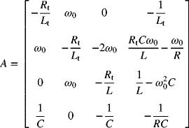
In an islanded mode, the VSC can employ an internal oscillator with a constant frequency ![]() to generate the modulation signals. As shown in Fig. 10.1, the control unit uses rated frequency and three-phase of PCC voltage to control the voltage. For the sake of linear robust control design, the linearized model of the MG is needed. The state space model of the system under balanced condition in abc-frame is given in (10.1), where
to generate the modulation signals. As shown in Fig. 10.1, the control unit uses rated frequency and three-phase of PCC voltage to control the voltage. For the sake of linear robust control design, the linearized model of the MG is needed. The state space model of the system under balanced condition in abc-frame is given in (10.1), where ![]() ,
, ![]() ,
, ![]() , and
, and ![]() are three-phase terminal voltage, terminal currents, PCC voltages, and PCC currents, respectively.
are three-phase terminal voltage, terminal currents, PCC voltages, and PCC currents, respectively.

Using α–β transformation and a rotating reference frame, which is presented in Ref. [20], the d- and q-axes of the state space variables system (Fig. 10.1) yield the following equations:

where
From (10.2), the transfer function of ![]() can be obtained as (10.3). The
can be obtained as (10.3). The ![]() and
and ![]() are direct voltage component of the PCC and inverter terminal voltage, respectively.
are direct voltage component of the PCC and inverter terminal voltage, respectively.
where ![]() , and
, and ![]() .
.
The N(s) and D(s) are numerator and denominator of the transfer function of the open-loop system, respectively. The ![]() ,
, ![]() ,
, ![]() ,
, ![]() ,
, ![]() ,
, ![]() , and
, and ![]() are numerator and denominator coefficients, which are expressed as follows:
are numerator and denominator coefficients, which are expressed as follows:

As seen from (10.3), the system has two zeroes and four poles. By substituting the rated values of system parameters given in the Table 10.1, the nominal transfer function of the plant, ![]() is obtained as expressed in Equation (10.4). The plant is minimum phase and stable for the nominal values (Table 10.1). However, parametric uncertainties, unpredictable generation variation, load disturbance, and faults may lead the MG to an unstable condition. A robust control may guarantee acceptable performance of the system in this circumstance.
is obtained as expressed in Equation (10.4). The plant is minimum phase and stable for the nominal values (Table 10.1). However, parametric uncertainties, unpredictable generation variation, load disturbance, and faults may lead the MG to an unstable condition. A robust control may guarantee acceptable performance of the system in this circumstance.
Table 10.1 Rated Values for the System Parameters
10.1.1.2 Controller Design
Bode diagrams of the open-loop system are shown in Fig. 10.2. The system gain margin and phase margin are 3.34 dB and 0.0241°, respectively; this indicates a relatively poor stability for the present case study. Based on Kharitonov's theorem [19], a polynomial such as K(s),
with real coefficients is Hurwitz if and only if the following four extreme polynomials are Hurwitz.

Figure 10.2 Open-loop Bode diagram of the system.
The ![]() and
and ![]() show the minimum and maximum bounds on the polynomial coefficients, respectively. In Kharitonov's theorem, the K(s) is a characteristic equation of the closed-loop system.
show the minimum and maximum bounds on the polynomial coefficients, respectively. In Kharitonov's theorem, the K(s) is a characteristic equation of the closed-loop system.
It is shown [19] that for polynomials with lower than fifth order, there are simpler criteria than (10.6). For a fifth-order plant, it is only sufficient to check the stability of ![]() ,
, ![]() , and
, and ![]() polynomials. For the problem at hand, the Kharitonov's theorem must be applied on the characteristic equation of the closed-loop system. Considering (10.3) with PI feedback control, the characteristic equation of the closed-loop system can be obtained as follows:
polynomials. For the problem at hand, the Kharitonov's theorem must be applied on the characteristic equation of the closed-loop system. Considering (10.3) with PI feedback control, the characteristic equation of the closed-loop system can be obtained as follows:
where
Here, ![]() and
and ![]() are coefficients of the open-loop transfer function system and,
are coefficients of the open-loop transfer function system and, ![]() and
and ![]() are proportional and integral gains of the PI controller, respectively. According to (10.7), the order of the closed-loop system is 5. Therefore, it is just needed to test the Hurwitz criteria for the following three polynomials:
are proportional and integral gains of the PI controller, respectively. According to (10.7), the order of the closed-loop system is 5. Therefore, it is just needed to test the Hurwitz criteria for the following three polynomials:

It is assumed that with ±10% change in rated values of the system parameters, the coefficients of the open-loop system (10.3) can be perturbed in the following ranges:
Following some manual algebraic operations to stabilize (10.8), a set of nine inequalities [4] is obtained. The resulting inequalities are satisfied for some ![]() and
and ![]() , which are presented in Fig. 10.3.
, which are presented in Fig. 10.3.
Figure 10.3 Acceptable values of Kp and Ki to stabilize the polynomials given in (10.8).
In addition to robust stability, to ensure a robust performance such as desirable time response, minimum overshoot/undershoot, and oscillation damping, it is important to maintain the roots of the characteristic equation in a specific region (D region). As seen from Fig. 10.3, there are numerous pairs of ![]() and
and ![]() . Using the D-stability concept, proper pairs of
. Using the D-stability concept, proper pairs of ![]() and
and ![]() , which remain the roots of the characteristic equation in a specific region are selected. Using this approach, the PI control parameters are tuned as
, which remain the roots of the characteristic equation in a specific region are selected. Using this approach, the PI control parameters are tuned as ![]() and
and ![]() .
.
The basic geometry associated with the zero exclusion condition [19] for ![]() is fully demonstrated in Fig. 10.4. The designed PI controller is robust if and only if the rectangle plots do not include the origin. This issue is confirmed in Fig. 10.4. By substituting values of
is fully demonstrated in Fig. 10.4. The designed PI controller is robust if and only if the rectangle plots do not include the origin. This issue is confirmed in Fig. 10.4. By substituting values of ![]() and
and ![]() in (10.7), the characteristic polynomial of the closed-loop system is determined as follows:
in (10.7), the characteristic polynomial of the closed-loop system is determined as follows:
Figure 10.4 The Kharitonov's rectangles: (a) for 0 < ω < 50 kHz and (b) a magnified view around the origin.
The closed-loop response of the MG system is evaluated against severe step load disturbances, changes in parameters, and operating mode. The simulation results are given in Ref. [4]. It is shown that the proposed control method can handle all test scenarios, effectively.
10.1.2 Intelligent Droop-Based Voltage and Frequency Control [3]
An intelligent method for droop control in an islanded MG based on neuro-fuzzy control technique is presented in Ref. [3]. With an appropriate training, this method can prevent the MG from instability and collapse in the presence of violent changes of load or outage of the distributed generation resource.
The neuro-fuzzy control structure is designed to maintain the system stability and minimizing voltage and frequency fluctuations regardless of the MG type and its structure. The most important advantage of the proposed controller is its independence from the MG structure and its operating condition. The participation percentage of active and reactive power in droop-based voltage and frequency controls are conventionally determined by the inductivity and resistivity characteristic of the lines. Based on the resistivity or inductivity of the MG, it is possible to illustrate the effective rate of active and reactive powers in voltage and frequency changes [3]. Since the variation of the load (consumption power) affects voltage and frequency simultaneously, the droop control P/f and Q/V cannot be analyzed, independently.
The main problem of the conventional droop control structure method is in their dependency to the line parameters. Here, an adaptive neuro-fuzzy inference system (ANFIS) is introduced for accurately estimation of these parameters [3].
10.1.2.1 Neuro-Fuzzy Control Framework
The artificial neural network (ANN) is one of the intelligent algorithms that can be used in both identification and control. The ANNs have the ability to learn system behavior and are effectively used for the identification of nonlinear dynamic systems. On the other hand, fuzzy logic (FL) is a powerful tool in control engineering, which can be used to control variable structure systems in the real-time world. The ANNs can be trained by the training data, but the FL has no ability for training. Combining FL and ANNs leads to a useful and valuable result.
Adding the training ability of ANN to FL creates a new hybrid technique, known as ANFIS. In this method, the correction of fuzzy rules is possible when the system is being trained, and by setting the ANN appropriately, previous knowledge about the membership function (MF) and rules is not required, and the optimum MFs are sufficient for obtaining the input/output (I/O) data. The configuration of MFs depends on their parameters. The ANFIS selects these parameters automatically, and does not need a human to obtain these parameters. The parameters of the membership functions are set by means of a back-propagation (BP) algorithm and the least-squares error (LSE) method.
The overall structure of an ANFIS unit is shown in Fig. 10.5 [3], which includes five layers. Weights of the MFs are analyzed in the first layer, which is known as the MF layer. In this layer, the input variables are applied to the MFs. The output of the second layer is the multiplication of the input signals, which are equivalent to IF rules. In the third layer, which is known as the rule base layer, the activity level of even rule is calculated. The number of layers is equal to the number of fuzzy rules. The output of this layer is a normalized form of the previous layer. The fourth layer obtains the output values of the resulting rules. This layer is known as the defuzzification layer. Finally, the output value of the system is obtained from the output layer.

Figure 10.5 Overall structure of an ANFIS.
Here, a generalized droop control (GDC) concept [3] is modeled by means of ANFIS, and the validity of the model is examined. Design steps can be summarized as follows:
- By applying and testing the GDC on the system shown in Fig. 10.6, and then saving the controller inputs/outputs, the training data for the ANFIS controller synthesis are collected. To obtain an accurate model, the training data under violent changes of active and reactive loads are considered.
- After obtaining the training data set, the ANFIS structure is completed. The MFs of input and output are considered in the form of linear and Gaussian functions.
- After creating the controller structure, using the optimal hybrid method (combination of the LSE and BP), the ANFIS is trained for 5 epochs (iterations) with a small error tolerance (i.e., 0.00001 ms).

Figure 10.6 A simple MG.
10.1.2.2 Synthesis Procedure and Performance Evaluation
A simple voltage source inverter (VSI)-based MG, shown in Fig. 10.6, is used for designing/training of the ANFIS controller. The ANFIS model is created by using the GDC. The GDC, which is introduced in Ref. [3], consists of two inputs (active and reactive power) and two outputs (voltage and frequency). Since one output is allowed for the construction of ANFIS in the related toolbox in MATLAB software, two ANFIS blocks are used as shown in Fig. 10.7.

Figure 10.7 The inputs and outputs of the proposed ANFIS controller.
Therefore, the considered functions for each block consist of two inputs and one output. After generating the I/O data set and applying them to the ANFIS toolbox, the model is trained. Here, to reconstruct the system behavior effectively, the switching frequency of the inverter is fixed at 4000 Hz, and the simulation sampling time is considered as 100,000 samples per second. To evaluate the performance of the designed ANFIS model, two sets of data are selected from the real data and training data (as the test data). These two sets are compared and the results are shown in Fig. 10.8. Comparing the real and network data shows whether the training process is done accurately. Figure 10.9 shows the closed-loop control system for a VSI-based inverter.

Figure 10.8 (a) Trained network output versus real output and (b) trained network output and real output together.

Figure 10.9 A VSI-based MG with ANFIS controller.
Two trained ANFIS controllers are replaced with the GDC [3]. After that, under the violent changes of active and reactive loads, the voltage and frequency of the closed-loop system are examined and compared with the generalized droop control structure. The applied scenario for active and reactive power changes is shown in Fig. 10.10a. Figure 10.10b shows the voltage and frequency profiles for both ANFIS and GDC-based methodologies. This figure shows the validity of the ANFIS controller with a high level of accuracy.
Figure 10.10 (a) Load change pattern scenario and (b) system response.
To prove the reliability of the closed-loop system with the designed ANFIS controller, it is also tested on several MG systems. The results are given in Ref. [3].
10.2 Secondary Control Synthesis
10.2.1 Intelligent Frequency Control [2]
The MGs mostly use renewable energy in electrical power production that vary naturally. These changes and usual uncertainties in power systems cause the classic controllers to be unable to provide a proper performance over a wide range of operating conditions. In response to this challenge, an online intelligent approach using a combination of the fuzzy logic and the particle swarm optimization (PSO) techniques for optimal tuning of the most popular existing PI-based frequency controllers in the AC MG systems is addressed in Ref. [2]. The control design methodology is examined on an isolated AC MG case study. The performance of the proposed intelligent control synthesis is compared with the pure fuzzy PI and the conventional Ziegler–Nichols method-based PI control designs.
10.2.1.1 Case Study
An isolated AC MG system is considered as the case study, which is shown in Fig. 10.11. The MG system contains conventional diesel engine generator (DEG), photovoltaic (PV) panel, wind turbine generator (WTG), fuel cell (FC) system, battery energy storage system (BESS), and flywheel energy storage system (FESS). As shown in Fig. 10.11, the DGs are connected to the MG by power electronic interfaces, which are used for synchronization in the AC sources like DEG and WTG and to reverse voltage in the DC sources like PV panel, FC, and energy storage devices.
Figure 10.11 Single-line diagram of the AC MG case study.
Each microsource has a circuit breaker to disconnect from the network to avoid the impacts of severe disturbances through the MG or for maintaining purposes. To easily understand the MG frequency response, a simplified frequency response model is given in Fig. 10.12. The FC contains three fuel blocks, an inverter for converting DC to AC voltage, and an interconnection device. Although the FC and some other DGs have high-order characteristic models, for the present study the introduced model (Fig. 10.12) is sufficient.
Figure 10.12 Simplified AC MG frequency response model.
This model can be useful to analyze/demonstrate the frequency behavior of the case study. The system details including PV and WTG models and the case study parameters are given in Ref. [2]. Since most of the energy sources have an intermittent nature with considerable uncertainty and fluctuation in the power system, efficient control methods must be employed to decrease the undesirable dynamic impacts.
10.2.1.2 Conventional and Fuzzy PI-Based Frequency Control
In traditional power systems, the secondary frequency control is mostly done by using conventional PI controllers that are usually tuned based on the specified operating points. In case of any change in the operating condition, the PI controllers cannot provide the assigned desirable performance. On the other hand, if the PI controller is able to track the changes that occur in the power system, the optimum performance will be always achieved. Fuzzy logic can be used as an intelligent method for online tuning of PI controller parameters.
In this section, the traditional PI controller for secondary frequency control is tuned by the well-known Ziegler–Nichols method. Then, a pure fuzzy PI controller is also designed. The result will be compared with the online PSO-fuzzy-based PI design methodology. A comprehensive study on classical PI/PID tuning methods like Ziegler–Nichols has been presented in Ref. [21]. Using the Ziegler–Nichols method, the PI parameters are obtained as given in Table 10.2.
Table 10.2 PI Control Parameters Using the Ziegler–Nichols Method
| Controller Parameter | Value |
| 4.095 | |
| 21.84 |
As described before, to achieve better performance, fuzzy logic is used as an intelligent method. Fuzzy logic is able to respond to the inability of the classic control theory for covering complex systems with their uncertainties and inaccuracies. The control framework for the application of the fuzzy logic system as an intelligent unit in order to fine-tune the traditional PI controller is shown in Fig. 10.13. The fuzzy PI controller has two levels: the first one is a traditional PI controller and the second one is a fuzzy system. As shown, the intelligent fuzzy system unit uses frequency deviation and load perturbation inputs to adjust the PI control parameters. In order to apply the fuzzy logic to the isolated MG system for tuning the PI control parameters, a set of fuzzy rules consisting of 18 rules is used to map input variables, ![]() (frequency deviation) and
(frequency deviation) and ![]() (load perturbation), to output variables,
(load perturbation), to output variables, ![]() (proportional gain) and
(proportional gain) and ![]() (integral gain).
(integral gain).

Figure 10.13 Fuzzy PI-based secondary frequency control.
The set of fuzzy rules are given in the Table 10.3 where membership functions corresponding to the input and output variables are arranged as negative large (NL), negative medium (NM), negative small (NS), positive small (PS), positive medium (PM), and positive large (PL). They have been arranged using the triangular membership function, which is the most traditional one. The antecedent parts of each rule are composed by using AND function (with interpretation of minimum). Here, the Mamdani fuzzy inference system is also used.
Table 10.3 The Fuzzy Rules Set
| Δf | ||||||
| NL | NM | NS | PS | PM | PL | |
| S | NL | NM | NS | PS | PS | PM |
| M | NL | NL | NM | PS | PM | PM |
| L | NL | NL | NL | PM | PM | PM |
It is shown that the fuzzy-based PI performance highly depends on the membership functions [3]. Without precise information about the system, the membership functions cannot be carefully selected, and the designed fuzzy PI controller does not provide optimal performance in a wide range of operating conditions. Therefore, a complementary algorithm is used for online regulation of membership functions.
10.2.1.3 PSO-Fuzzy PI Frequency Control
Here, for online tuning of membership functions employed in the fuzzy PI controller, the PSO is used. The PSO is an optimization algorithm, based on the probability laws, which is inspired by the natural models. This algorithm belongs to a class of direct search methods and is used to find an optimal solution for the optimization problems in a given search space. The applied PSO algorithm is extensively explained in Ref. [2].
Up to now, many search algorithms have been proposed in order to solve the optimization problems, including genetic algorithm, ant colony, and bee colony. However, simplicity is an important advantage of the PSO in comparison with other methods, especially genetic algorithm. Several modifications have been proposed to improve the performance of the PSO algorithm. According to the description provided, what this research investigates is designing an online adaptive controller, using fuzzy logic and PSO, for the purpose of frequency regulation in an AC MG system. The overall control framework for online adjusting of membership functions for the fuzzy rules based on the PSO technique is shown in Fig. 10.14.

Figure 10.14 Closed-loop system with PSO-fuzzy PI controller.
Considering the purpose of the algorithm, which is to find the extremum point of the cost function, if the cost function is not properly selected, the algorithm will be stopped in the local extremum points. Initialization of the algorithm parameters is also very important because if they are not carefully selected, the algorithm will never be convergent to the extremum point. The computational flow chart for the proposed online PSO-based optimal design approach is shown in Fig. 10.15.

Figure 10.15 The online PSO algorithm flowchart [2].
10.2.1.4 Simulation Results
To compare the classic, fuzzy PI and the PSO-fuzzy PI controllers, several simulation tests are carried out and the performances of the proposed control methods are evaluated. To illustrate the dynamic response of the MG system, the closed-loop system is examined in the face of a multiple step load disturbance, which is plotted in Fig. 10.16a. The MG frequency response using the conventional fuzzy PI and PSO-fuzzy PI (optimal PI) controllers is also shown in Fig. 10.16b.

Figure 10.16 (a) Multiple step load disturbances and (b) MG frequency response.
![]() and
and ![]() are MG frequency deviation and load disturbance, respectively, having values in “pu.” As shown, the proposed optimal PSO fuzzy PI controller regulating the system frequency following a disturbance is quite better than the pure fuzzy PI and classical PI controllers. For the sake of a clear comparison between the performance of the PSO-fuzzy PI and fuzzy PI controllers, system frequency following a severe step load disturbance of 0.1 pu is shown in the Fig. 10.17. In this case also, the proposed optimal control method provides a much better performance.
are MG frequency deviation and load disturbance, respectively, having values in “pu.” As shown, the proposed optimal PSO fuzzy PI controller regulating the system frequency following a disturbance is quite better than the pure fuzzy PI and classical PI controllers. For the sake of a clear comparison between the performance of the PSO-fuzzy PI and fuzzy PI controllers, system frequency following a severe step load disturbance of 0.1 pu is shown in the Fig. 10.17. In this case also, the proposed optimal control method provides a much better performance.

Figure 10.17 Frequency control following 0.1 pu step load disturbance.
Power system parameters are constantly changing and this may degrade the closed-loop system performance seriously. As indicated in the previous sections, one of the main advantages of the intelligent control methods is robustness against environmental and dynamical changes. To show the adaptive property of the PSO-fuzzy PI controller, the main power system parameters, in the frequency response model (Fig. 10.12), that is, D (damping coefficient), H (inertia constant), R (droop constant), ![]() (turbine time constant),
(turbine time constant), ![]() (generator time constant),
(generator time constant), ![]() (FESS time constant), and
(FESS time constant), and ![]() (BESS time constant) are significantly changed according to Tables 10.4 and 10.5.
(BESS time constant) are significantly changed according to Tables 10.4 and 10.5.
Table 10.4 Uncertain Parameters and Variation Range
| Parameter | Variation Range | Parameter | Variation Range |
| R | +30% | +50% | |
| D | −40% | −45% | |
| H | +50% | +55% | |
| −50% |
Table 10.5 Uncertain Parameters and Variation Range
| Parameter | Variation Range | Parameter | Variation Range |
| R | −60% | −62% | |
| D | −55% | −35% | |
| H | +48% | −50% | |
| −53% |
The closed-loop frequency response after applying these changes to the MG system parameters are shown in Figs. 10.18 and 10.19, respectively. It can be seen the conventional controller cannot handle the applied parameters perturbation. Figure 10.19 shows that the difference between the proposed optimal PSO-fuzzy PI controller with the other two controllers is more significant for a higher range of parameter variation.
Figure 10.18 Frequency response according to the parameter change (Table 10.4).

Figure 10.19 Frequency response according to the parameter change (Table 10.5).
Finally, two scenarios are examined for the secondary frequency control issue. First, only the DEG is considered as the responsible unit for frequency control in which the results are shown in the previous figures. The impact of the FC contribution in the secondary frequency control is considered as the second scenario. The output of the PSO-fuzzy PI controller is divided between the DEG and the FC units according to their participation factors. The result of this cooperation framework using the proposed intelligent technique is shown in Fig. 10.20.

Figure 10.20 Frequency deviation in case of contribution of both FC and DEG in frequency control.
10.2.2 ANN-Based Self-Tuning Frequency Control [5]
Like the conventional generating units, droop control is one of the important control methods for an MG with multiple DG units. The DG units must automatically adjust their set points using the frequency measurement to meet the overall need of the MG. However, unlike large power systems, the drooping system is poorly regulated in the MGs to support spinning reserve as an ancillary service for secondary frequency control. The main challenge is to coordinate their actions so that they can provide the regulation services.
The possibility of having numerous controllable DG units and MGs in distribution networks requires the use of intelligent, optimal, and hierarchical control schemes that enable an efficient control and management of this kind of systems. Generally, for the sake of control synthesis, nonlinear systems such as MGs are approximated by reduced order dynamic models, possibly linear, that represent the simplified dominant systems' characteristics. However, these models are only valid within specific operating ranges, and a different model may be required in the case of changing operating conditions. On the other hand, due to the increase of nonlinearity and complexity of MG systems, classical and nonflexible control structures may not represent a desirable performance over a wide range of operating conditions. Therefore, more flexible and intelligent approaches are needed [22].
The scheduling of the droop coefficients for frequency regulation in the MGs using an ANN is presented in Ref. [5]. Simulation studies are performed to illustrate the capability of the proposed optimal control approach. The resulting controllers are shown to minimize the effect of disturbances and achieve acceptable frequency regulation in the presence of various load change scenarios.
10.2.2.1 ANN in Intelligent Control
Neural networks are formed by neurons. An ANN is a crude approximation to parts of the real brain. It is just a parallel computational system consisting of many simple processing elements connected together in a specific way in order to perform a particular task. The ANNs provide a very important tool in optimization tasks because they are extremely powerful computational devices with the capability of parallel processing, learning, generalization, and fault/noise tolerating. Based on configuration and connecting elements, there are several main applications in ANNs such as brain modeling, financial modeling, time series prediction, control systems, and optimization.
Indeed, an ANN consists of a finite number of interconnected neurons (as described earlier) and acts as a massively parallel distributed processor, inspired from biological neural networks, which can store experimental knowledge and makes it available for use. To use neural networks in optimization tasks, it is needed to have a mathematical model of neural networks. A simplified mathematical model of a neuron is given in (10.10). It consists of three basic components that include weights ![]() , threshold (or bias)
, threshold (or bias) ![]() , and a single activation function
, and a single activation function ![]() .
.
The values ![]() ,
, ![]() ,…,
,…, ![]() are weight factors associated with each node to determine the strength of input row vector
are weight factors associated with each node to determine the strength of input row vector ![]() . Each input is multiplied by the associated weight of the neuron connection. Depending upon the activation function, if the weight is positive, the resulting signal commonly excites the output node; whereas, for negative weights, it tends to inhibit the output node. The node's internal threshold
. Each input is multiplied by the associated weight of the neuron connection. Depending upon the activation function, if the weight is positive, the resulting signal commonly excites the output node; whereas, for negative weights, it tends to inhibit the output node. The node's internal threshold ![]() is the magnitude offset that affects the activation of the output node y as follows [22]:
is the magnitude offset that affects the activation of the output node y as follows [22]:
The neurons could be combined together and they form a layer. Layers are constituted together and make a network. Updating the weights and training of neural networks is based on two basic feed-forward and feedback process. There are three methods for training the weights in feedback process: supervised, unsupervised, and reinforcement learning [22].
In supervised learning, the output is compared with the desired reference vector, and then error vectors applied for updating the weights. There is no desired reference vector for the reinforcement method and a revolutionary process is usually used for updating the weights. In the unsupervised learning method, updating is only based on the input data. In control structures, the supervised learning is usually used. There are several methods for supervised learning such as perceptron, Widrow–Hoff, correlation, and back-propagation learning methods. The most employed method is the back-propagation learning.
The main objective of intelligent control is to implement an autonomous system that could operate with increasing independence from human actions in an uncertain environment. The most common ANN-based intelligent control structures are well explained in Ref. [22]. In all existing structures, the control objectives could be achieved by learning from the environment through a feedback mechanism. The ANN has the capability to implement this kind of learning.
10.2.2.2 Proposed Control Scheme
The schematic diagram of the proposed control scheme for the ANN-based self-tuning frequency controller is shown in Fig. 10.21, where the ANN unit acts as an intelligent unit for optimal tuning of classic PI controller parameters, by getting input and output data based on certain rules. In the proposed intelligent control scheme, the ANN collects information about the plant (MG) response, adjusts weights via a learning algorithm, and recommends an appropriate control signal. In Fig. 10.21, the ANN performs an online automatic optimal tuner for the existing PI controller. The main components of the ANN as a fine-tuner for the PI controllers include a response recognition unit to monitor the controlled response and extract knowledge about the performance of the current controller gain setting, and an embedded unit to suggest suitable changes to be made to the controller gains.

Figure 10.21 Block diagram of the proposed control method.
The employed neural network structure for tuning the parameters of the PI controller used for frequency control (of the system given in Fig. 10.11) is shown in Fig. 10.22. In the ANN structure of Fig. 10.22, 20 linear neurons are considered for network input layer; 10 and 2 nonlinear neurons are also considered for hidden layer and output layer, respectively. The number of output layer's neurons is equal to the number of control parameters that must be adjusted. In Fig. 10.22, X is the input vector and W1 and W2 are connecting weight vectors between the layers.

Figure 10.22 The ANN structure used for PI tuning.
Selection of initial conditions in an ANN-based control system is also known as an important issue. In multiobjective control problems, some initial values may not guarantee the achievement of objectives with a satisfactory value of the optimization function. The initial conditions are usually selected according to the a priori information about distributions at the already-known structure of the open-loop ANN and selected control strategy. Here, the initial quantities in the applied ANN scheme (Fig. 10.22) are considered as follows:

As mentioned, linear functions are considered for the first layer, and for the second and third layers, the sigmoid functions are chosen. In the output layer, different coefficients for sigmoid function are considered for tuning of the controller parameters. The main advantage of using these nonlinear functions is in performing a smooth updating of weights.
The learning process of the applied ANN for the MG test system is to minimize the performance function given by (10.11), where yd represents reference signal and y represents the output of output layer.
The implemented algorithm for updating weights is based on back-propagation learning, which is described in the flowchart of Fig. 10.23. In the feed-forward process, by using the input vector (X), the values of hidden layer output (H) and output layer result (O) are provided, and then error value (E) obtained from the process is employed to update the weights as follows:
where ![]() is a learning rate given by a small positive constant, and
is a learning rate given by a small positive constant, and

Figure 10.23 Flowchart of updating weights via back-propagation learning.
The learning process continues to reach the desired minimum error. This method is presented in detail in Ref. [22]. For testing of the proposed control methodology for tuning the PI controller parameters, the controller is applied to the case study (Fig. 10.11), and the results are compared with the response of a conventional PI controller.
To examine the proposed control strategy, system frequency response in the presence of the ANN-based self-tuning PI controller and conventional PI controller is tested. Here, a random step load disturbance, WTG mechanical output power variations, and sunlight flux variations are simultaneously considered in the MG test system to better evaluate the proposed closed-loop control performance. In this scenario, it is assumed that the BESS and FESS systems do not participate in the secondary frequency control issue. The results for the first scenario are plotted in Fig. 10.24a–e.

Figure 10.24 System response: (a) step load disturbances, and WTG and PV power, (b) WTG power, (c) PV power, (d) DEG power, and (e) system frequency.
The considered power fluctuations, the WTG and PV output power variations, the DEG frequency response, and system frequency are shown in Fig. 10.24a–e, respectively. As shown, only the DEG participates in the secondary frequency control process and it injects more compensating power by using the proposed intelligent control method. Therefore, when the ANN adjusts the controller parameters, system frequency fluctuations are much less.
10.3 Global Control Synthesis
As a considerable capability, each MG can operate in autonomous (isolated from the main grid) and grid-connected modes. The performance measure in the autonomous mode is the reliability of stand-alone operation. However, in the grid-connected mode the MG operates while connected to the main grid. This is especially characterized by the fact that each MG can sell a portion of its generated power to the grid at a point of connection and at the same time is able to purchase a portion of its demand from the grid at another point of connection. As a result of power sharing in this mode, load demand supplement is guaranteed at all times by the grid.
The increasing amount of demand for electrical energy along with growing environmental concerns motivate the idea of establishing new power systems with flexible and intelligent programs of generation as well as demand-side management. These programs run by utility companies aim to provide consumers with a reliable and cost-efficient energy and at the same time to make efficient use of the generation and transmission infrastructure. While many of these programs are still under investigation, there already exist a number of practical applications in many countries across the world.
In this direction, energy consumption scheduling and power dispatching can be considered as important global control issues in distribution networks with interconnected MGs
10.3.1 Adaptive Energy Consumption Scheduling [7]
Demand side can be managed by either reducing or shifting the consumption of energy. While the former can be efficient to some extent, the latter proposes shifting of high load household consumptions to off-peak hours in order to reduce peak-to-average ratio (PAR). The high PAR might lead to degradation of power quality, voltage problems, and even potential damages to utility and consumer equipment.
With the advancement of smart metering technologies and increasing interest in power distribution networks with two-way communications capability, load management has appeared in the form of energy consumption scheduling (ECS). In the ECS, the power consumption time of connected units is optimally scheduled so that some interesting measures such as generation cost and PAR can be optimized efficiently. This results in reducing the risk of getting into a condition that may lead to a blackout. As an incentive that subscribers follow ECS decisions, intelligent pricing schemes in the form of lower utility charges should be provided.
Consequently, customers will be encouraged to shift their heavy loads to off-peak hours. These issues motivate the design of ECS with the aim of minimizing power generation cost and PAR. The proposed ECS schemes in the literature mainly perform network-wide load management with the assumption of the knowledge of the whole network demand a priori or at least with known statistical characteristics. In other words, a network operator should be aware of the whole network demand in some way. Due to the diversity of power customers ranging from household to industrial domains with uncertain demands, however, this case is not mostly valid. Alternatively, an operator who is aware of demand in a local area, not other neighbor areas, might be interested in ECS within this area. The fact that aggregate power generation cost depends on the network-wide demand necessitates considering the impact of uncertain demands in the design of the ECS.
To investigate the mentioned difficulty, a distribution network connecting to a local area (LA) consisting of several MGs with known demand in average and other neighbor areas (NAs) with uncertain demands is considered. The network operator performs ECS of demand in the LA considering NAs demand as a random variable. This ECS is formulated with two stochastic optimization problems, one with the objective of the network-wide power generation cost minimization and the other with the objective of PAR minimization. While these two objectives are correlated to some extent, optimizing one does not necessarily imply the optimality of the other.
These objectives are compared using optimal, adaptive, and uniform scheduling schemes in terms of generation cost and PAR. In the optimal one, the optimal solutions of two underlying problems are achieved with the assumption of the knowledge of NAs demand in advance. Without this assumption for practical purposes, an adaptive scheme with online stochastic iterations to capture the randomness of uncertain demands over the time horizon continually is proposed. Finally, in uniform scheduling, the demand of MGs in LA is uniformly distributed over the time horizon regardless of NAs demand.
10.3.1.1 Distribution Network with Connected MGs
A simplified architecture of a distribution network organized by a distribution company (Disco1) is shown in Fig. 10.25. This network consists of N connected MGs in an LA, and NAs that may belong to another company (Discoi). The microsources and storage devices use power electronic circuits to connect to the MG. The MG can be connected to the network by a PCC via a static switch. This switch is capable of islanding the MG for maintenance purposes or when faults or a contingency occurs.
Figure 10.25 A distribution network with connected MGs.
The DNO deals with some overall responsibilities for the distribution network (Disco) and the connected MGs, such as interchange power between the main grid and the MGs. This unit, which is located in the application layer of the distribution management system is acting in an economically based energy management between the main grid and the neighboring MGs.
As shown in Fig. 10.25, the DNO interfaces the main grid (Disco1) with the connected MGs (in the LA) as well as other neighbor grids (in NAs that may be covered by another Disco). The DNO also supervises the power flow control and market operation. This operator controls power flow from the main grid to the MGs to keep it close to the scheduled values. In the mentioned network, identifying the optimal consumption/generation schedule to minimize production costs and to balance the demand and supply, as well as online assessment of security and reliability, are the responsibilities of the DNO unit. As mentioned in Chapter 9, the DNO together with the MGCCs supervise the MG's market activities such as buying and selling active and reactive power to the grid and possible network congestions for transferring energy from a distribution network to the MGs in a local area and other neighboring areas.
10.3.1.2 Proposed Methodology and Results
Pricing of electricity can be used as a mechanism to encourage customers to follow a specified load scheduling. Various pricing schemes have been proposed by economists and regulatory agencies such as flat pricing, critical-peak pricing, time-of-use pricing, and real-time pricing. Among them, real-time pricing is motivated to be used in the next-generation power systems concerning its environmental and economic gains. Accordingly, in the present work, an energy scheduling approach based on real-time generation cost is proposed, which can be used to establish a real-time pricing scheme.
In the mentioned network, the objective of DNO to implement ECS could be either to minimize power generation cost or to minimize PAR. A solution is summarized as an adaptive cost-aware ECS (ACA-ECS) algorithm [7]. In order to minimize PAR of the total instantaneous power delivered to LA and NAs during the time period T, a minmax formulation is proposed with the objective of minimizing the peak of this power. The mathematical formulations are given in Ref. [7].
For investigation of the proposed methods, a distribution network is considered in connection with an LA consisting of N = 10 MGs and an NA. The ECS located in the DNO schedules energy consumption of MGs in LA during a time horizon of length 6 h.
The impact of the proposed ACA–ECS algorithm on the time domain curvature of the total grid demand in the presence of an unknown NA demand is evaluated and the result is compared with an optimal technique. A typical realization of T = 360 samples of NA demand with standard deviation of σ = 20 kWh and the corresponding optimal total demand are shown in Fig. 10.26a. As observed, the optimal solution schedules LA demand such that the system-wide total demand becomes smooth suitable for cost minimization. In fact, scheduling the LA demand provides a diversity for the ECS to mitigate the stochastic nature of NA demand. Total demand using the ACA–ECS scheme and the corresponding Lagrange multipliers [7] are also shown in Fig. 10.26b. Intuitively, after some initial time slots, the behavior of the total demand curve approximately converges to that of the optimal solution in Fig. 10.26a.

Figure 10.26 Simulation results: (a) generated NAs demand and the system-wide optimal demand, (b) adaptive system-wide demand and Lagrange multipliers, (c) generation cost per kWh in cost formulation, (d) PAR in cost formulation, (e) generation cost per kWh in the PAR formulation, and (f) PAR in PAR formulation.
Performance measures of the ACA–ECS and the optimal ECS schemes, such as generation cost per kWh and PAR, versus the randomness of the NA demand could be interesting in the following. As another scheduling scheme, the results of uniform ECS scheme are also included. In this scheme, the demand of each MGn in LA is uniformly distributed over the whole time horizon, independent of the NA demand. This can also be considered as a deterministic solution. Cost and PAR performances versus the standard deviation are shown in Fig. 10.26c and d, respectively. For each instance, similar to the time-domain performance, first a data set with T = 360 samples are generated. This set is used to obtain the optimal ECS solution once in the beginning of the time horizon as well as to provide the ACA–ECS scheme with instantaneous realized NA demand. As shown in the first part of Fig. 10.26a, there is a typical generated data set with σ = 20 kWh. As a common observation in Fig. 10.26c and d, performance measures get worse as σ increases. In the case of cost measure, this is due to the fact that the considered squared cost function results in higher cost per kWh for high demand values in comparison with low demand values. The results in PAR are based on the fact that the averages of both LA and NA demands are made constant when σ increases. Considering PAR as a fractional term of the peak demand over the average demand, it is reasonable to conclude that PAR increases as σ increases. Moreover in Fig. 10.26c, with increase in σ, the performance gap between the compared ECS schemes and the optimal one increases. In the case of ACA–ECS, this is due to the fact that the stochastic estimator (given in Ref. [7]) would be far from optimality with the increase in the randomness of the uncertain part of power generation. In the case of uniform ECS, the degradation effect of high randomness would be more severe since this scheme does not take care of NA demand in the scheduling decisions.
Furthermore, in Fig. 10.26c and d, the generation cost and PAR performances of the ACA–ECS scheme outperform those of uniform ECS. This is reasonably expected as ACA–ECS takes advantage of the diversity in NA demand to smooth the total demand and therefore achieves a better performance. In the comparison between ACA–ECS and the optimal solution, it is observed that the optimal solution achieves lower cost. This is due to the fact that this solution fully takes into account the knowledge of NA demand at the beginning of the time horizon for the scheduling of LA demand. However, ACA–ECS makes a scheduling decision adaptively per a time unit, when the demand of NA is available in that unit. Remarkably, the PAR of ACA–ECS is comparable to that of the optimal solution. This implies that the optimality of generation cost does not necessarily imply the optimality of PAR too. This observation motivates the performance evaluation of PAR formulation in the following.
In order to evaluate the efficiency of PAR formulation, the generation cost per kWh and PAR performances of this formulation are illustrated in Fig. 10.26e and f, respectively. Similar to the cost formulation [7], the results of optimal solution in PAR formulation (optimal PAR) and uniform scheduling (uniform PAR) scheme are also included. Since the scheduling of the uniform strategy is independent of the objective function, the achieved results are the same in both cost and PAR formulations. We take advantage of this equality and take uniform strategy curves as references for comparison between these formulations.
Comparing Fig. 10.26c and e, it is observed that uniform scheduling was the worst in the former, whereas it is the best in the latter. Considering the results of uniform scheduling as reference in both figures, we conclude that cost minimization formulation is more cost efficient in comparison with PAR formulation. In terms of PAR, the optimal solution in the PAR formulation achieves the lowest PAR. This is reasonably expected as this solution takes NA demand into account a priori. In comparison with the uniform strategy, the PAR of PAR–ECS scheme is high. More importantly, this implies that PAR performance of the proposed adaptive approach in cost minimization formulation even outperforms its equivalent in the PAR minimization formulation.
This observation along with the lower generation cost in cost formulation demonstrates that our proposed adaptive approach achieves more efficient results with this formulation compared with the PAR one. Also, the proposed adaptive approach is a trade-off between the optimal (full NAs demand) and uniform (no NAs demand) schemes in terms of generation cost and PAR minimization.
10.3.2 Power Dispatching in Interconnected MGs [8]
Load demand management is a critical issue in the smart grids with power sharing capability. It controls the power dispatching between MGs with the aim of establishing a balance between power supply and demand in a cost-efficient manner. The objective in this balance is to alleviate peak loads at individual MGs and accordingly avoids major expenditures in power utilities. In contrast to the autonomous mode where load management results in shifting peak loads to off-peak loads, peak loads of an MG in grid-connected mode can be handled by the means of power sharing throughout the grid.
Considering stochastic demands and maximum allowed supplies in MGs, an immediate question is how to perform power dispatching and to set interactions in the grid. Due to power generation and transmission costs, this issue raises the economic exploitation of the resources within the grid. The outcome of power dispatching could be interesting in this perspective.
In Ref. [8], load demand management of an electric network of interconnected MGs is formulated as a power dispatch optimization problem. Real-time pricing is employed as a motivation for interactions between the MGs. The objective is to minimize the network operational cost and at the same time to satisfy the stochastic demands within the MGs in average. With the solution of this problem, a cooperative power dispatching algorithm between MGs is proposed under the assumption of a communication infrastructure within the grid. The core parameter in this algorithm is a defined dynamic purchase price per unit of power at each MG. Considering their demands and supplies, the MGs progressively update and broadcast their prices throughout the grid. Every MG adaptively regulates its transactions with the rest of the grid by taking into account its realized demand as well as already announced prices from the other MGs. This strategy results in a semidistributed and reliable load management within the grid in a cost-efficient manner.
10.3.2.1 Methodology and Results
As an example, consider a power grid consisting of small MGs starting from MG1 and ending with MG8 as shown in Ref. [8]. The distance between any two neighbor MGs is the same and is noted as one hop. The transmission price per unit of power between any two MGs is assumed to be the number of hops between them. Moreover, the power generation function is assumed to be a square function.
The simulation is run for 200 time slots; each slot with realization of a new demand and new maximum permitted supply values per MG. Produced powers at individual MGs by the proposed statistical cooperative power dispatching (SCPD) algorithm are shown in Fig. 10.27a. The sn in this figure represents the produced power of MGn. Despite the diverse power demands, the produced powers are close to each other. In comparison with their demands, low demand MGs produce higher power and high demand ones produce lower power. This is due to the fact that low demand MGs tend to sell power, whereas high demand ones tend to purchase power. Figure 10.27b illustrates Lagrange multipliers λi by which MGs interact within the grid. As previously mentioned, each λi in the SCPD algorithm can be interpreted as the price that announces at time slot to pay for a unit of power from any other MG in the system. As shown, even though all prices are initialized with the same value, they statistically converge to different levels during the simulation. The higher is the demand, the higher is the announced price for power purchasing.

Figure 10.27 Simulation results: (a) MGs produced powers over time, (b) announced power prices over time, (c) average load demands, and produced, sold and purchased powers, and (d) cost comparison between grid-connected SCPD and autonomous modes.
The curves in this figure are interpreted relative to each other, that is, power flow direction within the grid is from MGs with low prices to ones with high prices. In other words, an MG with low purchase price in comparison with others is an indication of power selling and vice-versa.
The average demand, produced, sold, and purchased powers of individual MGs in the SCPD algorithm are shown in Fig. 10.27c. While demand increases linearly with MG indexes in accordance with assumed values, produced powers are approximately the same for all MGs, in compliance with Fig. 10.27a. Remarkably, the sum of produced and purchased powers at each MG is equal to the sum of demand plus sold power. This reveals the energy balance within the grid. Purchased and sold power curves vary in opposite directions versus the MG index, that is, purchased power increases with demand, whereas sold power decreases. Exceptionally, the decrease of purchased power is possibly due to its location in the network topology, which burdens high power transmission cost. In a logical statement, low demand MGs sell power to high demand ones.
This statement is investigated by comparing the average operational costs at individual MGs in these two modes, shown in Fig. 10.27d. To this end, the cost in autonomous mode is obtained from the square power production function. Furthermore, the cost in grid-connected mode implemented by SCPD algorithm is the production cost plus purchased cost minus the revenue from selling power to the other MGs. As shown, the grid-connected mode achieves lower cost for low demand and high demand MGs. The decrease in the cost of low demand MGs is the result of selling power to high demand ones. In particular, the cost of MG1 and MG2 even get negative as a result of high revenue from selling power that compensates their production cost. This outcome also decreases the cost of high demand MGs as they purchase a portion of their demand from the low demand ones. This is accomplished by means of high announced purchase prices in Fig. 10.27b. Furthermore, the purchased and sold power of moderate demand MGs are mostly the same. In summary, as a numerical indicator, the proposed SCPD in the grid connected mode achieves 20% cost reduction in comparison with stand-alone operation. Overall, this power sharing scheme transforms the parabolic cost curve to a linear one as shown in Fig. 10.27d.
10.4 Emergency Control Synthesis
Like conventional systems, having acceptable voltage and frequency levels is necessary in an MG. In grid-connected mode, this issue is realized by the main grid because distributed generators are often based on active and reactive power (P–Q) controlled inverters with specific amount of active and reactive powers. However, in islanded mode, the MG security strongly depends on the capability of existing MG controllers in primary, secondary, and emergency levels. Also, power exchange between the main grid and MG in a grid-connected mode leads to voltage and frequency variations during transient between two operation modes. Stable performance of the MG in the transient and islanding states is dependent on the VSI-based DGs.
As mentioned before, after disconnection the control mode of one or several DGs will change from the P–Q control to the VSI control. However, this control may be unable to stabilize an islanded MG following large disturbances like load disturbance and generator trip, which change the balance between generation and consumption. In such cases, emergency control may need to be activated. In this section, an effective load shedding (LS) scheme based on both voltage and frequency records as the last action to prevent the system blackout is suggested.
10.4.1 Developed LS Algorithm [10,11]
The proposed LS algorithm is summarized in a flowchart, which is shown in Fig. 10.28. The LS scheme uses both frequency and voltage measurements as well as the rate of change of frequency (ROCOF). Here, the amount of voltage decrease following a disturbance is used to determine the number of load blocks to be shed; therefore, voltage parameter is measured at first. Any significant change in voltage causes the algorithm to be started. However, to prevent unnecessary LS, frequency and ROCOF are also measured during the specified recording time window (e.g., τ s). If they pass the determined thresholds, the LS will be initiated.

Figure 10.28 The LS algorithm.
Amount of frequency and ROCOF thresholds can be defined based on a fault condition in which only one load block is required to be shed. On the other hand, the amount of voltage reduction determines the severity of disturbance/fault. The number of load blocks for the LS is calculated from a look-up table. This table is determined based on voltage deviation range following disturbances. Recording of voltage drop for different events and performing of a look-up table can be achieved by increasing loads until the system is stabilized by eliminating all needful load blocks for the LS.
When the LS is initiated, the removal of the first group of load blocks (N) will be done from the look-up table. However, it may need to shed more blocks following a delay due to breakers operation. After T seconds, the frequency is measured again to ensure that it is not reaching its nominal value. This process will be continued until the frequency returns to the nominal value.
10.4.2 Case Study and Simulation
Here, a simple MG which is used in [23], is considered as the case study. The base voltage of the MG is 13.8 kV, which is connected to a 69 kV distribution grid through a substation transformer and breaker. The system includes four feeders and three DGs. Two electronically interfaced DGs (DG2 and DG3) and one conventional unit (DG1) are located in feeders 3, 4, and 1, respectively. It is assumed that the available loads are divided into critical and noncritical RL loads. The noncritical loads are shed in the necessary conditions.

Figure 10.29 System response after using the LS scheme: (a) MG frequency and (b) bus voltages.
The proposed LS plan is applied to the case study, following loss of DG2 at t = 0.7 s. Simulation results show that after this disturbance and islanding, the MG system becomes unstable. Therefore, the LS is required to stabilize the islanded MG system. Here, based on dynamical knowledge obtained mainly via simulations, the look-up table (Table 10.6) is performed and the required thresholds are determined.
Table 10.6 Look-Up Table of Load Shedding
| Voltage Deviation Range, pu | Number of Load Blocks for LS (N) |
| V ≥ 0.776 | 0 |
| 0.776 < V ≤ 0.733 | 1 |
| 0.733 < V ≤ 0.71 | 2 |
| 0.71 < V ≤ 0.696 | 3 |
| 0.696 < V ≤ 0.68 | 4 |
| 0.68 < V ≤ 0.67 | 5 |
| V ≤ 0.67 | All load blocks for load shedding |
Following this disturbance, the voltage decreases to 0.774 pu. According to the look-up table, the number of load blocks (N) for LS is 1. Therefore, one block is shed at t = 0.886 s. After T and delay time, the frequency goes back to the normal range. This means that it is not necessary to shed more load blocks. The system response due to the use of the proposed LS is presented in Fig. 10.29.
In an islanded MG that has reached equilibrium after islanding, the voltage of all buses and branches changes following a disturbance. If a generation unit is tripped all branch voltages will decrease, except the related branch of the removed generator. At the moment of separation, voltage owned the branch of the tripped unit increases and remains constant at this value. This voltage increase in any branch of generation unit is the sign of loss of that unit.
It is noteworthy that an LS is impressionable by the location of shed loads. However, whenever the amount of load blocks to be shed is more the effect of location is less. In the Fig. 10.29, the load with first priority was shed.
10.5 Summary
This chapter addresses several synthesis methodology examples for controller design in an MG. These examples cover all control levels, that is, primary, secondary, global, and emergency controls. The applied algorithms and control techniques are mostly based on robust, intelligent, and optimal/adaptive strategies.
References
- 1. H. Bevrani and T. Hiyama, Frequency regulation in isolated systems with dispersed power sources. In: Intelligent Automatic Generation Control, CRC Press, New York, 2011, Chapter 12, pp. 263–277.
- 2. H. Bevrani, F. Habibi, P. Babahajyani, M. Watanabe, and Y. Mitani, Intelligent frequency control in an AC microgrid: on-line PSO-based fuzzy tuning approach, IEEE Trans. Smart Grid, 3 (4), 1935–1944, 2012.
- 3. H. Bevrani and S. Shokoohi, An intelligent droop control for simultaneous voltage and frequency regulation in islanded microgrids, IEEE Trans. Smart Grid, 4 (3), 1505–1513, 2013.
- 4. F. Habibi, A. H. Naghshbandy, and H. Bevrani, Robust voltage controller design for an isolated microgrid using Kharitonov's theorem and D-stability concept, Int. J. Electr. Power, 44, 656–665, 2013.
- 5. H. Bevrani, F. Habibi, and S. Shokoohi, ANN-based self-tuning frequency control design for an isolated microgrid. In: P. Vasant, editor, Meta-Heuristics Optimization Algorithms in Engineering, Business, Economics, and Finance, IGI Global, Hershey, PA, 2012, Chapter 12, pp. 357–385.
- 6. P. Babahajyai, F. Habibi, and H. Bevrani, An on-line PSO-based fuzzy logic tuning approach: microgrid frequency control case study. In: P. Vasant, editor, Handbook of Research on Novel Soft Computing Intelligent Algorithms: Theory and Practical Applications, IGI Global, Hershey, PA, 2014, Chapter 20, pp. 589–616.
- 7. M. Fathi and H. Bevrani, Adaptive energy consumption scheduling for connected microgrids under demand uncertainty, IEEE Trans. Power Deliv., 28 (3), 1576–1583, 2013.
- 8. M. Fathi and H. Bevrani, Statistical cooperative power dispatching in interconnected microgrids, IEEE Trans. Sustain. Energy, 4 (3), 586–593, 2013.
- 9. H. Bevrani, M. Gholami, and N. Hajimohammadi, Microgrid emergency control and protection: key issues and new perspectives, Int. J. Energy Optim. Eng., 2 (1), 78–100, 2013.
- 10. N. Hajimohammadi and H. Bevrani, Load shedding in microgrids. In: 21st Iranian Conference on Electrical Engineering (ICEE-2013), Mashad, Iran, 2013.
- 11. N. Hajimohammadi and H. Bevrani, On load shedding design in microgrids. In: 18th Electric Power Distribution Conference, Kermanshah, Iran, April 30–May 1, 2013.
- 12. S. Shokoohi, H. Bevrani, and A. H. Naghshbandi, Application of neuro-fuzzy controller on voltage and frequency stability in islanded microgrids. In: Conference on Smart Electric Grids Technology (SEGT2012), Tehran, Iran, December 18–19, 2012, pp. 62–67.
- 13. A. H. Naghshbandi, S. Shokoohi, and H. Bevrani, Application of neuro-fuzzy controller on voltage and frequency stability in islanded microgrids, J. Electr. Eng., 41 (2), 41–49, 2011.
- 14. M. Fathi and H. Bevrani, Adaptive price-based power flow in next generation electric power systems. In: International Symposium on Smart Grid Operation and Control (ISSGOC 2012), Sanandaj, Iran, 2012.
- 15. H. Bevrani and T. Ise, Virtual synchronous generators: a survey and new perspectives, Technical Report, Osaka University, Osaka, Japan, 2012.
- 16. P. Babahajyani, F. Habibi, and H. Bevrani, An on-line PSO-based fuzzy logic tuning approach: microgrid frequency control case study. In: International Symposium on Smart Grid Operation and Control (ISSGOC 2012), 2012.
- 17. F. Habibi, S. Shokoohi, and H. Bevrani, Designing a self-tuning frequency controller using ANN for an isolated microgrid. In: International Symposium on Smart Grid Operation and Control (ISSGOC 2012), 2012.
- 18. S. Shokoohi and H. Bevrani, PSO based droop control of inverter interfaced distributed generations. In: Conference on Smart Electric Grids Technology (SEGT2012), Tehran, Iran, December 18–19, 2012, pp. 77–82.
- 19. B. R. Barmish, New Tools for Robustness of Linear Systems, Macmillian, New York, 1994.
- 20. F. Karimi, E. J. Davison, and R. Iravani, Multivariable servomechanism controller forautonomous operation of a distributed generation unit: design and performance evaluation, IEEE Trans. Power Syst., 25 (2), 853–865, 2010.
- 21. D. Xue, Y. Q. Chen, and D. P. Atherton, Linear Feedback Control: Analysis and Design with MATLAB, Vol. 14, Society for Industrial and Applied Mathematics, 2007.
- 22. H. Bevrani and T. Hiyama, Intelligent Automatic Generation Control, CRC Press, New York, 2011.
- 23. F. Katiraei and M. R. Iravani, Power management strategies for a microgrid with multiple distributed generation units, IEEE Trans. Power Syst., 21 (4), 1821–1831, 2006.