To illustrate, let’s consider another business application of classification: targeting online display advertisements to consumers, based on what webpages they have visited in the past. As consumers, we have become used to getting a vast amount of information and services on the Web seemingly for free. Of course, the “for free” part is very often due to the existence or promise of revenue from online advertising, similar to how broadcast television is “free.” Let’s consider display advertising—the ads that appear on the top, sides, and bottom of pages full of content that we are reading or otherwise consuming.

Display advertising is different from search advertising (e.g., the ads that appear with the results of a Google search) in an important way: for most webpages, the user has not typed in a phrase related to exactly what she is looking for. Therefore, the targeting of an advertisement to the user needs to be based on other sorts of inference. For several chapters now we have been talking about a particular sort of inference: inferring the value of an instance’s target variable from the values of the instance’s features. Therefore, we could apply the techniques we already have covered to infer whether a particular user would be interested in an advertisement. In this chapter we introduce a different way of looking at the problem that has wide applicability and is quite easy to apply.

Let’s define our ad targeting problem more precisely. What will be an instance? What will be the target variable? What will be the features? How will we get the training data?

Let’s assume that we are working for a very large content provider (a “publisher”) who has a wide variety of content, sees many online consumers, and has many opportunities to show advertisements to these consumers. For example, Yahoo! has a vast number of different advertisement-supported web “properties,” which we can think of as different “content pieces.” In addition, recently (as of this writing) Yahoo! agreed to purchase the blogging site Tumblr, which has 50 billion blog posts across over 100 million blogs. Each of these might also be seen as a “content piece” that gives some view into the interests of a consumer who reads it. Similarly, Facebook might consider each “Like” that a consumer makes as a piece of evidence regarding the consumer’s tastes, which might help target ads as well.

For simplicity, assume we have one advertising campaign for which we would like to target some subset of the online consumers that visit our sites. This campaign is for the upscale hotel chain, Luxhote. The goal of Luxhote is for people to book rooms. We have run this campaign in the past, selecting online consumers randomly. We now want to run a targeted campaign, hopefully getting more bookings per dollar spent on ad impressions.^[50]

Therefore, we will consider a consumer to be an instance. Our target variable will be: did/will the consumer book a Luxhote room within one week after having seen the Luxhote advertisement? Through the magic of browser cookies,^[51] in collaboration with Luxhote we can observe which consumers book rooms. For training, we will have a binary value for this target variable for each consumer. In use, we will estimate the probability that a consumer will book a room after having seen an ad, and then, as our budget allows, target some subset of the highest probability consumers.

We are left with a key question: what will be the features we will use to describe the consumers, such that we might be able to differentiate those that are more or less likely to be good customers for Luxhote? For this example, we will consider a consumer to be described by the set of content pieces that we have observed her to have viewed (or Liked) previously, again as recorded via browser cookies or some other mechanism. We have many different kinds of content: finance, sports, entertainment, cooking blogs, etc. We might pick several thousand content pieces that are very popular, or we may consider hundreds of millions. We believe that some of these (e.g., finance blogs) are more likely to be visited by good prospects for Luxhote, while others (e.g., a tractor-pull fan page) are less likely.

However, for this exercise we do not want to rely on our presumptions about such content, nor do we have the resources to estimate the evidence potential for each content piece manually. Furthermore, while humans are quite good at using our knowledge and common sense to recognize whether evidence is likely to be “for” or “against,” humans are notoriously bad at estimating the precise strength of the evidence. We would like our historical data to estimate both the direction and the strength of the evidence. We next will describe a very broadly applicable framework both for evaluating the evidence, and for combining it to estimate the resulting likelihood of class membership (here, the likelihood that a consumer will book a room after having seen the ad).

It turns out that there are many other problems that fit the mold of our example: classification/class probability estimation problems where each instance is described by a set of pieces of evidence, possibly taken from a very large total collection of possible evidence. For example, text document classification fits exactly (which we’ll discuss next in Chapter 10). Each document is a collection of words, from a very large total vocabulary. Each word can possibly provide some evidence for or against the classification, and we would like to combine the evidence. The techniques that we introduce next are exactly those used in many spam detection systems: an instance is an email message, the target classes are spam or not-spam, and the features are the words and symbols in the email message.

We are interested in quantities such as the probability of a consumer booking a room after being shown an ad. We actually need to be a little more specific: some particular consumer? Or just any consumer? Let’s start with just any consumer: what is the probability that if you show an ad to just any consumer, she will book a room? As this is our desired classification, let’s call this quantity C. We will represent the probability of an event C as p(C). If we say p(C) = 0.0001, that means that if we were to show ads randomly to consumers, we would expect about 1 in 10,000 to book rooms.^[52]

Now, we are interested in the probability of C given some evidence E, such as the set of websites visited by a particular consumer. The notation for this quantity is p(C|E), which is read as “the probability of C given E,” or “the probability of C conditioned on E.” This is an example of a conditional probability, and the “|” is sometimes called the “conditioning bar.” We would expect that p(C|E) would be different based on different collections of evidence E—in our example, different sets of websites visited.

As mentioned above, we would like to use some labeled data, such as the data from our randomly targeted campaign, to associate different collections of evidence E with different probabilities. Unfortunately, this introduces a key problem. For any particular collection of evidence E, we probably have not seen enough cases with exactly that same collection of evidence to be able to infer the probability of class membership with any confidence. In fact, we may not have seen this particular collection of evidence at all! In our example, if we are considering thousands of different websites, what is the chance that in our training data we have seen a consumer with exactly the same visiting patterns as a consumer we will see in the future? It is infinitesimal. Therefore, what we will do is to consider the different pieces of evidence separately, and then combine evidence. To discuss this further, we need a few facts about combining probabilities.

Joint Probability and Independence

Let’s say we have two events, A and B. If we know p(A) and p(B), can we say what is the probability that both A and B occur? Let’s call that p(AB). This is called the joint probability.

There is one special case when we can: if events A and B are independent. A and B being independent means that knowing about one of them tells you nothing about the likelihood of the other. The typical example used to illustrate independence is rolling a fair die; knowing the value of the first roll tells you nothing about the value of the second. If event A is “roll #1 shows a six” and event B is “roll #2 shows a six”, then p(A) = 1/6 and p(B) = 1/6, and importantly, even if we know that roll #1 shows a six, still p(B) = 1/6. In this case, the events are independent, and in the case of independent events, p(AB) = p(A) · p(B)—we can calculate the probability of the “joint” event AB by multiplying the probabilities of the individual events. In our example, p(AB) = 1/36.

However, we cannot in general compute the probabilities of joint events in this way. If this isn’t clear, think about the case of rolling a trick die. In my pocket I have six trick dice. Each trick die has one of the numbers from one to six on all faces—all faces show the same number. I pull a die at random from my pocket, and then roll it twice. In this case, p(A) = p(B) = 1/6 (because I could have pulled any of the six dice out with equal likelihood). However, p(AB) = 1/6 as well, because the events are completely dependent! If the first roll is a six, so will be the second (and vice versa).

The general formula for combining probabilities that takes care of dependencies between events is:

Equation 9-1. Joint probability using conditional probability

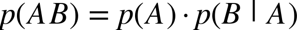
This is read as: the probability of A and B is the probability of A times the probability of B given A. In other words, given that you know A, what is the probability of B? Take a minute to make sure that has sunk in.

We can illustrate with our two dice examples. In the independent case, since knowing A tells us nothing about p(B), then p(B|A) = p(B), and we get our formula from above, where we simply multiply the individual probabilities. In our trick die case, p(B|A) = 1.0, since if the first roll was a six, then the second roll is guaranteed to be a six. Thus, p(AB) = p(A) · 1.0 = p(A) = 1/6, just as expected.

In general, events may be completely independent, completely dependent, or somewhere in between. If events are not completely independent, knowing something about one event changes the likelihood of the other. In all cases, our formula p(AB) = p(A) · p(B|A) combines the probabilities properly.

We’ve gone through this detail for a very important reason. This formula is the basis for one of the most famous equations in data science, and in fact in science generally.

Bayes’ Rule

Notice that in p(AB) = p(A)p(B|A) the order of A and B seems rather arbitrary—and it is. We could just as well have written:

This means:

And so:

If we divide both sides by p(A) we get:

Now, let’s consider B to be some hypothesis that we are interested in assessing the likelihood of, and A to be some evidence that we have observed. Renaming with H for hypothesis and E for evidence, we get:

This is the famous Bayes’ Rule, named after the Reverend Thomas Bayes who derived a special case of the rule back in the 18th century. Bayes’ Rule says that we can compute the probability of our hypothesis H given some evidence E by instead looking at the probability of the evidence given the hypothesis, as well as the unconditional probabilities of the hypothesis and the evidence.

Note: Bayesian methods

Bayes’ Rule, combined with the fundamental principle of thinking carefully about conditional independence, is the foundation for a large number of more advanced data science techniques that we will not cover in this book. These include Bayesian networks, probabilistic topic models, probabilistic relational models, Hidden Markov Models, Markov random fields, and others.

Importantly, the last three quantities may be easier to determine than the quantity of ultimate interest—namely, p(H|E). To see this, consider a (simplified) example from medical diagnosis. Assume you’re a doctor and a patient arrives with red spots. You guess (hypothesize) that the patient has measles. We would like to determine the probability of our hypothesized diagnosis (H = measles), given the evidence (E = red spots). In order to directly estimate p(measles|red spots) we would need to think through all the different reasons a person might exhibit red spots and what proportion of them would be measles. This is likely impossible even for the most broadly knowledgeable physician.

However, consider instead the task of estimating this quantity using the righthand side of Bayes’ Rule.

• p(E|H) is the probability that one has red spots given that one has measles. An expert in infectious diseases may well know this or be able to estimate it relatively accurately.
• p(H) is simply the probability that someone has measles, without considering any evidence; that’s just the prevalence of measles in the population.
• p(E) is the probability of the evidence: what’s the probability that someone has red spots—again, simply the prevalence of red spots in the population, which does not require complicated reasoning about the different underlying causes, just observation and counting.

Bayes’ Rule has made estimating p(H|E) much easier. We need three pieces of information, but they’re much easier to estimate than the original value is.

Note

p(E) may still be difficult to compute. In many cases, though, it does not have to be computed, because we are interested in comparing the probabilities of different hypotheses given the same evidence. We will see this later.

It is possibly quite obvious now that Bayes’ Rule should be critical in data science. Indeed, a very large portion of data science is based on “Bayesian” methods, which have at their core reasoning based on Bayes’ Rule. Describing Bayesian methods broadly is well beyond the scope of this book. We will introduce the most fundamental ideas, and then show how they apply in the most basic of Bayesian techniques—which is used a great deal. Let’s rewrite Bayes’ Rule yet again, but now returning to classification. Let’s for the moment emphasize the application to classification by writing out "C = c" — the event that the target variable takes on the particular value c.

Equation 9-2. Bayes Rule for classification

In Equation 9-2, we have four quantities. On the lefthand side is the quantity we would like to estimate. In the context of a classification problem, this is the probability that the target variable C takes on the class of interest c after taking the evidence E (the vector of feature values) into account. This is called the posterior probability.

Bayes’ Rule decomposes the posterior probability into the three quantities that we see on the righthand side. We would like to be able to compute these quantities from the data:

Estimating these three values from training data, we could calculate an estimate for the posterior p(C = c| E) for a particular example in use. This could be used directly as an estimate of class probability, possibly in combination with costs and benefits as described in Chapter 7. Alternatively, p(C = c| E) could be used as a score to rank instances (e.g., estimating those that are most likely to respond to our advertisement). Or, we could choose as the classification the maximum p(C = c| E) across the different values c.

Unfortunately, we return to the major difficulty we mentioned above, which keeps Equation 9-2 from being used directly in data mining. Consider E to be our usual vector of attribute values <e₁ , e₂ , ⋯, e_k>, a possibly large, specific collection of conditions. Applying Equation 9-2 directly would require knowing the p(E|c) as p(e₁ ∧ e₂ ∧ ⋯ ∧ e_k|c).^[53] This is very specific and very difficult to measure. We may never see a specific example in the training data that exactly matches a given E in our testing data, and even if we do it may be unlikely we’ll see enough of them to estimate a probability with any confidence.

Bayesian methods for data science deal with this issue by making assumptions of probabilistic independence. The most broadly used method for dealing with this complication is to make a particularly strong assumption of independence.

Conditional Independence and Naive Bayes

Recall from above the notion of independence: two events are independent if knowing one does not give you information on the probability of the other. Let’s extend that notion ever so slightly.

Conditional independence is the same notion, except using conditional probabilities. For our purposes, we will focus on the class of the example as the condition (since in Equation 9-2 we are looking at the probability of the evidence given the class). Conditional independence is directly analogous to the unconditional independence we discussed above. Specifically, without assuming independence, to combine probabilities we need to use Equation 9-1 from above, augmented with the |C condition:

However, as above, if we assume that A and B are conditionally independent given C,^[54] we can now combine the probabilities much more easily:

This makes a huge difference in our ability to compute the probabilities from the data. In particular, for the conditional probability p(E |C=c) in Equation 9-2, let’s assume that the attributes are conditionally independent, given the class. In other words, in p(e₁∧e₂∧⋯∧e_k|c), each e_i is independent of every other e_j given the class c. For simplicity of presentation, let’s replace C=c simply by c, as long as it won’t lead to confusion.

Each of the p(e_i | c) terms can be computed directly from the data, since now we simply need to count up the proportion of the time that we see individual feature e_i in the instances of class c, rather than looking for an entire matching feature vector. There are likely to be relatively many occurrences of e_i.^[55] Combining this with Equation 9-2 we get the Naive Bayes equation as shown in Equation 9-3.

Equation 9-3. Naive Bayes equation

This is the basis of the Naive Bayes classifier. It classifies a new example by estimating the probability that the example belongs to each class and reports the class with highest probability.

If you will allow two paragraphs on a technical detail: at this point you might notice the p(E) in the denominator of Equation 9-3 and say, whoa there—if I understand you, isn’t that going to be almost as difficult to compute as p(E |C)? It turns out that generally p(E) never actually has to be calculated, for one of two reasons. First, if we are interested in classification, what we mainly care about is: of the different possible classes c, for which one is p(C| E) the greatest? In this case, E is the same for all, and we can just look to see which numerator is larger.

In cases where we would like the actual probability estimates, we still can get around computing p(E) in the denominator. This is because the classes often are mutually exclusive and exhaustive, meaning that every instance will belong to one and only one class. In our Luxhote example, a consumer either books a room or does not. Informally, if we see evidence E it belongs either to c₀ or c₁. Mathematically:

Our independence assumption allows us to rewrite this as:

Combining this with Equation 9-3, we get a version of the Naive Bayes equation with which we can compute the posterior probabilities easily from the data:

Although it has lots of terms in it, each one is either the evidence “weight” of some particular individual piece of evidence, or a class prior.

Cumulative Response and Lift Curves presented the notion of lift as a metric for evaluating a classifier. Lift measures how much more prevalent the positive class is in the selected subpopulation over the prevalence in the population as a whole. If the prevalence of hotel bookings in a randomly targeted set of consumers is 0.01% and in our selected population it is 0.02%, then the classifier gives us a lift of 2—the selected population has double the booking rate.

With a slight modification, we can adapt our Naive Bayes equation to model the different lifts attributable to the different pieces of evidence. The slight modification is to assume full feature independence, rather than the weaker assumption of conditional independence used for Naive Bayes. Let’s call this Naive-Naive Bayes, since it’s making stronger simplifying assumptions about the world. Assuming full feature independence, Equation 9-3 becomes the following for Naive-Naive Bayes:

The terms in this equation can be rearranged to yield:

Equation 9-4. Probability as a product of evidence lifts

where lift_c(x) is defined as:

Consider how these evidence lifts will apply to a new example E =<e₁, e₂, ⋯, e_k>. Starting at the prior probability, each piece of evidence—each feature e_i—raises or lowers the probability of the class by a factor equal to that piece of evidence’s lift (which may be less than one).

Conceptually, we start off with a number—call it z—set to the prior probability of class c. We go through our example, and for each new piece of evidence e_i we multiply z by lift_c(e_i). If the lift is greater than one, the probability z is increased; if less than one, z is diminished.

In the case of our Luxhote example, z is the probability of booking, and it is initialized to 0.0001 (the prior probability, before seeing evidence, that a website visitor will book a room). Visited a finance site? Multiply the probability of booking by a factor of two. Visit a truck-pull site? Multiply the probability by a factor of 0.25. And so on. After processing all of the e_i evidence bits of E, the resulting product (call that z_f) is the final probability (belief) that E is a member of class c—in this case, that visitor E will book a room.^[56]

Considered this way, it may become clearer what the independence assumption is doing. We are treating each bit of evidence e_i as independent of the others, so we can just multiply z by their individual lifts. But any dependencies among them will result in some distortion of the final value, z_f. It will end up either higher or lower than it properly should be. Thus the evidence lifts and their combination are very useful for understanding the data, and for comparing instance scores, but the actual final value of the probability should be taken with a large grain of salt.

Let’s examine some evidence lifts from real data. To freshen things up a little, let’s consider a brand new domain of application. Researchers Michal Kosinski, David Stillwell, and Thore Graepel recently published a paper (Kosinski et al., 2013) in the Proceedings of the National Academy of Sciences showing some striking results. What people “Like” on the social-networking site Facebook^[57] is quite predictive of all manner of traits that usually are not directly apparent:

We encourage you to read the paper to understand their experimental design. You should be able to understand most of the results now that you have read this book. (For example, for evaluating how well they can predict many of the binary traits they report the area under the ROC curve, which you can now interpret properly.)

What we would like to do is to look to see what are the Likes that give strong evidence lifts for “high IQ,” or more specifically for scoring high on an IQ test. Taking a sample of the Facebook population, let’s define our target variable as the binary variable IQ>130.

So let’s examine the Likes that give the highest evidence lifts…^[58]

So, recalling Equation 9-4 above, and the independence assumptions made, we can calculate the lift in probability that someone has very high intelligence based on the things they Like. On Facebook, the probability of a high-IQ person liking Sheldon Cooper is 30% higher than the probability in the general population. The probability of a high-IQ person liking The Lord of the Rings is 69% higher than that of the general population.

Of course, there are also Likes that would drag down one’s probability of High-IQ. So as not to depress you, we won’t list them here.

This example also illustrates how it is important to think carefully about exactly what the results mean in light of the data collection process. The result above does not really mean that liking The Lord of the Rings is necessarily a strong indication of high IQ. It means clicking “Like” on Facebook’s page called The Lord of the Rings is a strong indication of a high IQ. This difference is important: the act of clicking “Like” on a page is different from simply liking it, and the data we have are on the former and not the latter.

Prior chapters presented modeling techniques that basically ask the question: “What is the best way to distinguish target values?” in different segments of the population of instances. Classification trees and linear equations both create models this way, trying to minimize loss or entropy, which are functions of discriminability. These are termed discriminative methods, in that they try directly to discriminate different targets.

This chapter introduced a new family of methods that essentially turns the question around and asks: “How do different target segments generate feature values?” They attempt to model how the data was generated. In the use phase, when faced with a new example to be classified, they use the models to answer the question: “Which class most likely generated this example?” Thus, in data science this approach to modeling is called generative. The large family of popular methods known as Bayesian methods, because they depend critically on Bayes’ Rule, are usually generative methods. The literature on Bayesian methods is both broad and deep, and you will encounter them often in data science.

This chapter focused primarily on a particularly common and simple but very useful Bayesian method called the Naive Bayes classifier. It is “naive” in the sense that it models each feature as being generated independently (for each target), so the resulting classifier tends to double-count evidence when features are correlated. Because of its simplicity it is very fast and efficient, and in spite of its naïveté it is surprisingly (almost embarrassingly) effective. In data science it is so simple as to be a common “baseline" method—one of the first methods to be applied to any new problem.

We also discussed how Bayesian reasoning using certain independence assumptions can allow us to compute “evidence lifts” to examine large numbers of possible pieces of evidence for or against a conclusion. As an example, we showed that the probability of “Liking” Fight Club, Star Trek, or Sheldon Cooper on Facebook each is about 30% higher for high-IQ people than for the general population.