
Using the ROC Curve to Evaluate Multivariable Prediction Models |
|

8.3 Resubstitution Estimate of the ROC Curve
8.4 Split-Sample Estimates of the ROC Curve
8.5 Cross-Validation Estimates of the ROC Curve
8.6 Bootstrap-Validated Estimates of the ROC Curve
8.1 Introduction
Our discussions so far have focused on a single predictor. Other variables were considered, such as when comparing several predictors or covariate-adjusted ROC curves, but not in the form of producing predictions from multivariable models and evaluating their accuracy. Chapters 8 and 9 deal with this problem.
It is useful to discuss the reasons for emphasizing single predictors. First, they provide the foundation for evaluating more complicated models. Second, single predictor applications are common in practice and thus deserve special focus. Diagnostic radiology is a good example where predictors are usually the products of patients undergoing scans. Although combining information from multiple sources of data (such as alternative diagnostic scans like magnetic resonance imaging and computed tomography) improves accuracy, the overwhelming financial and ethical concern is on minimizing the number of scans. This leads to concerns about picking the best single predictor out of a few candidates. Combining the information from multiple scan types is rarely of interest because the incremental improvement in accuracy does not usually justify the cost and burden for a patient to undergo additional diagnostic procedures.
Most prediction problems outside diagnostic radiology involve multiple variables. Usually, most outcomes of interest that you set out to predict are complex multidimensional entities that can be captured only through judicious use of several variables. This usually implies building a model, which requires choosing among several competing models. The goal of this process is finding the model that fits the data best, but it inevitably leads to over-fitting. Over-fitting refers to a model that describes the observed data much better than it anticipates future observations.
Measures of model performance (such as the ROC curve or the area under the ROC curve) that are computed from the data set used for model fitting are said to be obtained by self-prediction or resubstitution. These terms originate from the practice of using the model to predict the data that generated itself and resubstituting the model back into the data to obtain predictions. Another, somewhat light-hearted term for this method is double dipping, referring to the fact that the data set is used twice, once for fitting and once for predicting. The ROC curve and its summary measures tend to reflect the optimism in self-prediction because they indicate better accuracy than the actual model allows in practice.
Most statisticians recommend taking measures against over-fitting. This process is usually called validation. Here are two methods that are particularly relevant for ROC curves and that can be implemented in SAS with relative ease: split-sample validation and sample reuse validation. The sample reuse method can actually be implemented in two different ways: cross-validation and bootstrap. This chapter covers these methods.
Split-sample validation requires splitting the sample into two parts, so-called training and test sets. The model is fit on the training set and its performance is evaluated on the test set. This mimics the real-life situation where models are used on data sets that have not been part of the model development. Measures of performance estimated from the test set are much closer to the true values (less biased) than the ones estimated from the training set. Split-sample validation is simple to understand and implement. It also approximates real life well. Its main disadvantage is the inefficient use of data: with small to moderate sample sizes, neither the training nor the test sets are large enough to generate reproducible results.
Sample reuse methods attempt to increase efficiency by repeated use of observed data points in different ways. This repeated use results in estimators of performance with smaller variances. In general, however, because each data point is used more than once, there is an increase in bias. Nevertheless, most studies have favored sample reuse in terms of a composite criterion such as the mean squared error. In other words, the increase in bias is offset by the decrease in variance.
The most well-known sample reuse method is cross-validation. The data are divided into k segments (usually of equal size) and one part is set aside for testing while the remaining k–1 parts are used for training the model. Then this process is repeated for each segment and the resulting measures of accuracy are averaged over the k segments. When k=n, each data point constitutes a segment and the resulting process is called leave-one-out validation.
An alternative to cross-validation is to use bootstrap samples. We have seen in previous chapters how the bootstrap method can be used to obtain confidence intervals and p-values. When the goal is model validation, bootstrap samples obtained in the same way may be used to correct for over-fitting. Section 8.6 shows you how.
8.2 Liver Surgery Example
We will use a data set from the field of liver surgery throughout this chapter as an example. Surgery is the most promising treatment option for patients with liver cancer. The Liver data set has records from 554 surgeries that were performed to remove liver tumors. It is a subset of the data analyzed by Jarnagin et al. (2002). Variables include demographics, pre-operative patient characteristics such as existing co-morbid conditions, operative variables such as blood loss, and postoperative variables such as the incidence and severity of complications following the surgery.
Due to the nature of liver tumors, and aided by the fact that the liver has a unique ability to regenerate, most surgeries include removal of a substantial portion of the liver. This exposes patients to an elevated risk of complications. Predicting the likelihood of complications before surgery enables the treating team of physicians and nurses to increase post-operative monitoring of the patient as necessary. It is also helpful for counseling the patient and the patient's family.
We will use the following preoperative variables as potential predictors of post-operative complications: age, presence of any co-morbid conditions, extent of surgery (extensive vs. limited, where extensive is defined as an operation in which at least an entire lobe, or side, of the liver is resected), bilateral surgery (whether both lobes of the liver were involved in the resection or not), and number of segments resected (a segment is one of the eight anatomical divisions of the liver). Age and number of segments are considered as continuous variables. The typical number of resected segments is between 1 and 4, but occasionally 5 or 6 segments are taken out.
8.3 Resubstitution Estimate of the ROC Curve
The following code builds the predictions based on PROC LOGISTIC using a stepwise model selection method. Logistic regression is one of the many options available in SAS/STAT to build a predictive model for a binary outcome. Similarly, stepwise selection is one of several available model selection techniques. The goal here is not to claim logistic regression as the best way to build a predictive model, nor to promote stepwise as a model selection strategy. The emphasis is on model validation using several techniques.
This invocation of PROC LOGISTIC requests a model to be selected using the stepwise method. Stepwise selection enters variables one by one and then removes them as needed according to their level of statistical significance. The following is an algorithmic summary of stepwise selection:
- For each candidate variable, generate a p-value by adding the variable to the existing model from the previous step. In the first step, all variables in the model statement are candidates and the existing model is the intercept-only model.
- Choose the candidate variable with the highest significance (lowest p-value) and update the existing model with the addition of the chosen variable. If no variables meet the criterion for entry (p≤0.05 by default but can be tailored using the SLE option of the MODEL statement), then the existing model is considered final.
- Remove any variable that loses significance (p>0.05 by default but can be tailored using the SLS option of the MODEL statement) from the existing model. If several variables have lost significance, remove each variable one by one starting with the variable with the highest p-value. After each removal, p-values are regenerated by refitting the model. Return the removed variables to the list of candidates.
- At this point, all the variables in the existing model should be significant by the SLS criterion. All the other variables should be in the list of candidates. Go to Step 1 and repeat the process until none of the candidate variables are significant and none of the variables in the existing model can be removed.
Stepwise selection is a widely studied and somewhat controversial topic. It is used here to demonstrate the data-dependent nature of model selection and give a sense of how model selection procedures try to choose a model that provides the best fit to the data with little or no penalty for over-fitting. Although there are alternatives to or modifications of stepwise selection, generally, most forms of model selection lead to over-fit.
The relevant portion of the results appears in Output 8.1. The first table summarizes the stepwise selection. In this example, only two of the six variables were found to be significant: the number of segments resected and the age.
Output 8.1

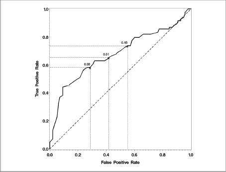
The familiar PROC LOGISTIC output indicates that this two-variable model has an AUC of 0.696, an estimate that we think is optimistic based on reasons described earlier. The ROC curve corresponding to this model is plotted in Figure 8.1. Of course, it is not just the area under the ROC curve that is overestimated; the estimated sensitivity for each value of specificity is optimistic, too.
Figure 8.1 Resubstitution Estimate of the ROC Curve for the Liver Resection Data

8.4 Split-Sample Estimates of the ROC Curve
Now, we'll see how to reduce the bias in resubstitution estimates using validation. The first step in split-sample validation is splitting the data set into two parts: training and test samples. They do not have to be of equal size. In fact, traditionally the training set is taken to be larger than the test set. A 2:1 split is commonly employed, where two-thirds of the observations are assigned to the training set and the remaining one-third to the test set. This split is usually done at random, although there are times when you might want to use a stratified split. A stratified split is one that ensures that proportionate amounts of one variable (or, at most, a few variables) appear in both training and test sets.
After the sample is split, the predictive model is built on the training set and estimates required for the ROC curve are obtained on the test set using the model optimized on the training set.
Splitting the sample can be done in many ways in SAS. The following DATA step is one example:
In this DATA step, a uniform random variable Unif is generated using the RANUNI function. Each observation is then assigned to either the training or test data set, depending on the corresponding realization of the Unif random variable. Essentially, the Unif variable represents a biased coin flip that determines whether the observation under consideration will be used for training the model or testing it.
The threshold for Unif is chosen as 0.333; therefore, approximately one-third of the records will have unif<0.333. Unif is a random variable, however, and each realization of this random variable produces a slightly different proportion of records where unif<0.333. For this reason, this method does not always produce an exact 2:1 match. If an exact 2:1 split is required, then you can sort the data on Unif first and then the desired number of records (in this example, exactly two-thirds of all records) for the training data can be taken from the beginning of the sorted sequence while the rest of the records are assigned to the test set. In most cases, an exact split is not necessary and the code given earlier will be sufficient.
After creating the training and test sets, the first task is to fit a model using the training data, as follows:
The primary difference in this call to PROC LOGISTIC is the OUTMODEL= option, which saves the details of the fitted model such as the parameter estimates and standard errors. The strength of the OUTMODEL= option is often more evident when it is combined with its sister option, INMODEL=, which accepts a model saved by the OUTMODEL= option as seen here:
Note the absence of a MODEL statement. This is because a new model fit is not desired. Instead, all the calculations are based on the model specified by the INMODEL= option. The SCORE statement generates predictions on the test data set using the model fit specified in the INMODEL= option. The OUT= option of the SCORE statement generates a data set that contains predicted probabilities in addition to all the original variables in the data set specified in the DATA= option.
At this point, you can use the techniques developed in Chapter 3 to plot an ROC curve using the %PLOTROC macro or you can compute the area under the curve using the %ROC macro. The ROC curve and the area under it generated from the test set are considered unbiased estimates of the true ROC curve and the AUC. The key observation is that the predicted probabilities obtained by the SCORE statement serve as the marker values. For example, the following call to the %ROC macro produces the split-sample estimate of the AUC curve (see Output 8.2), which turns out to be 0.677, roughly 0.02 less than the resubstitution estimate of 0.696, illustrating the optimism in the resubstitution estimates:
Output 8.2

Note that P_1 is the variable name assigned to the predictions by the SCORE statement.
It is also possible to plot the split-sample ROC curve using the %PLOTROC macro introduced in Chapter 3. Since P_1 is given to several significant digits, a new variable P1 is created in the data set TESTSCORE to facilitate printing of thresholds. P1 is created as follows:
P1 = ROUND(P_1,0.01);
Then the following invocation of %PLOTROC is used:
Figure 8.2 Split-Sample Estimate of the ROC Curve Using the %PLOTROC Macro
Note that thresholds in Figure 8.2 are described in terms of predicted probabilities because the marker plotted is the predicted probability from the logistic model (see MARKER= in the %PLOTROC macro call).
As an alternative to the %PLOTROC macro, you can use the OUTROC= option of the SCORE statement, which generates a data set that is identical in structure to the OUTROC= option in the MODEL statement. Specifically, it contains the variables _SENSIT_ and _1MSPEC_, which can be used in a PLOT statement of a call to PROC GPLOT.
Finally, it is instructive to overlay the resubstitution and split-sample estimates. This is accomplished in Figure 8.3, which shows the two ROC curves, one obtained by resubstitution and one by split-sample validation. The resubstitution curve is above the split-sample curve for the most part, but there are regions where the split-sample curve rises above the resubstitution curve. This seems contrary to the expectation that all the points on the ROC curve will be overestimated by resubstitution. This highlights the primary disadvantage of the split-sample approach; namely, it provides only one test set on which estimates of accuracy (such as sensitivity at a given specificity) can be computed. Although it provides unbiased estimates, they contain considerable variability and a situation like the one we have just observed is not uncommon. This is the primary reason for using the sample reuse methods discussed in the next two sections.
Figure 8.3 Comparison of the Resubstitution and Split-Sample Estimates of the ROC Curve for the Liver Resection Example

8.5 Cross-Validation Estimates of the ROC Curve
8.5.1 Leave-One-Out Estimation
PROC LOGISTIC offers a built-in option for cross-validation, which performs the leave-one-out method. As briefly explained in the introduction to this chapter, the leave-one-out method works by setting aside an observation, building a model on the rest of the data set, and then using the model to predict the left-out record. When this process is repeated for each observation, a prediction is obtained for every record in the data set using a model that was blind to the predicted observation. These predictions form the basis for a cross-validated ROC curve.
Leave-one-out cross-validation can be performed by PROC LOGISTIC using the following code. The PREDPROBS=X option in the OUTPUT statement specifies that leave-one-out cross-validation be used instead of resubstitution. This option applies to all the predicted probabilities generated by the OUTPUT statement. If the PREDPROBS= option is omitted, predicted probabilities are calculated using resubstitution.
Now the ROC curve can be plotted using the same methods recommended for split-sample validation, including one of the plotting macros. The area under the ROC curve and its standard error can be obtained through the %ROC macro. The following call to the %ROC macro produces the leave-one-out estimate of the AUC (Output 8.3), using the data set created by PROC LOGISTIC at the time the PREDPROBS=X option is specified. The variable name of the cross-validated predicted probability is XP_1:
Output 8.3

The estimate of the AUC, as obtained by leave-one-out cross-validation, is 0.6875 with confidence limits (0.6431–0.7318). Figure 8.4 contrasts the resubstitution estimate of the ROC curve and the leave-one-out estimate of the ROC curve. Although the two curves are very close, the leave-one-out estimate is consistently below the resubstitution estimate.
Figure 8.4 Comparison of the Resubstitution and Leave-One-Out Estimates of the ROC Curve for the Liver Resection Example
It may at first seem reasonable to use the OUTROC= option in this example to plot the ROC curve. However, the PREDPROBS=X option does not affect the data set created by the OUTROC= option in the MODEL statement. Even if you specify the OUTROC= and PREDPROBS=X options at the same time, the data set created by the OUTROC= option still reports the resubstitution estimates. Similarly, measures of association including c and Somers' D are also reported on a resubstitution basis. Therefore, the usual ways of obtaining ROC points and the area under the curve are not applicable for cross-validation, and these tasks have to be performed manually outside PROC LOGISTIC.
8.5.2 K-Fold Cross-Validation
While specifying the PREDPROBS=X option is a convenient way to obtain leave-one-out estimates, you should learn more about how cross-validation can be performed in SAS using the %XVAL macro. You can perform k-fold cross-validation using this macro. It is also helpful when making predictions with other procedures, such as the PROBIT, GENMOD, or GAM procedures, which do not offer standard cross-validation options.
The starting point for k-fold cross-validation involves breaking up the data in k randomly chosen segments, where k is a number supplied by the user. With k-fold cross-validation, the analyses are repeated k times. For each analysis, one of the k segments is left out as the test set and the remaining k–1 are used for training. In each analysis, the model is blinded to the test data. Table 8.1 explains the role of each segment cross-validation in the special case of k=5.
Table 8.1 The Role of Segments within Each Analysis in Five-Fold Cross-Validation

There are a few advantages to this schema of validation:
- It is conceptually simple.
- Each segment (hence, each data point because segments are nonoverlapping) appears exactly once in the test set, so one and only one prediction is made for each data point.
- The choice of k allows for some flexibility in adjusting the size of the training and test sets.
The second point forms the basis of validation for our purposes. You can obtain an ROC curve directly from these predicted values since there is one prediction for each observation in the data set. This can be achieved by using any of the methods described in the previous section since, from the standpoint of obtaining ROC curves, there is no difference between a data set obtained by using the SCORE statement in PROC LOGISTIC and the test data combined from the k analyses from k-fold cross-validation.
The %XVAL macro, which is available from the book's companion Web site at support.sas.com/gonen, performs cross-validation. K is an input to the macro, along with the data set name, outcome, and covariates. The %XVAL macro produces no output but generates a data set called _XVAL_, which contains cross-validated predicted probabilities (P_0 and P_1=1−P_0) in addition to the original variables. This resulting data set can be used in calls to the %PLOTROC and %ROC macros to obtain cross-validated estimates of the ROC curve and the area under it. For example, these three macro calls perform a five-fold cross-validation for the Liver data:
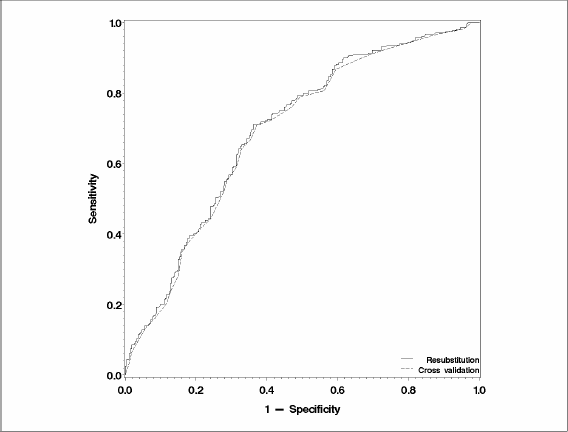
The ROC curve generated by the %PLOTROC macro appears in Figure 8.5 and the results from the %ROC macro appear in Output 8.4. The estimate of the five-fold validated AUC is 0.6883, with a standard error of 0.0226, virtually indistinguishable from the leave-one-out estimates.
Figure 8.5 Five-Fold Cross-Validated Estimates of the ROC Curve

Output 8.4

The need for cross-validation extends beyond linear logistic models fit by PROC LOGISTIC. Other SAS procedures that accept similar data but use different methods to fit models, such as PROC GENMOD, PROC GAM, and PROC PROBIT, can also benefit from cross-validation schema. It is difficult to write one general-purpose macro that will work with all the procedures because each one has different output syntax and Output Delivery System (ODS) table names. But it is relatively easy to tailor the %XVAL macro for different procedures. The initial DATA step in the macro adds a variable XV to the data set, which takes values from 1 to K, indicating which fold the observation belongs to. This portion is independent of the statistical prediction model or the SAS procedure used. You must modify the parts of the code that use PROC LOGISTIC. This modification requires procedure-specific expertise and may be accomplished by users who have experience with the particular procedure and with macro programming.
8.6 Bootstrap-Validated Estimates of the ROC Curve
Another sample reuse method of obtaining an ROC curve by validation is using bootstrap samples. This is not as intuitive as cross-validation, but it may, in certain cases, have a lower variance associated with estimation.
Bootstrap validation begins by forming B bootstrap samples. While for cross-validation, K was a small number (on the order of 5 to 10), for bootstrap validation, B will typically be larger, at least several hundred or perhaps 1,000. Each bootstrap sample is then used as a training sample. Then the original data set and the bootstrap sample are used as test samples. The difference between the measure of interest (say, the AUC) estimated from using the original data as the test sample and the measure of interest estimated from using the bootstrap sample as the test sample is a measure of optimism. This difference can be subtracted from the resubstitution estimate of the measure of interest to obtain the bootstrap-validated estimate. Estimates produced this way are sometimes called optimism-corrected or optimism-adjusted estimates.
The algorithm follows:
| 1. | Compute the measure of interest, M, on the original data set, call it Mo. |
| 2. | Create B bootstrap samples. For i=1,…B, do the following: |
| a. | Train a model on the bootstrap sample |
| b. | Compute M using the trained model on the original data; call it Moi |
| c. | Compute M using the trained model on the bootstrap sample; call it Mbi |
| d. | Compute the difference: di= Moi− Mbi |
| 3. | Subtract the mean(di) from Mo. This is the bootstrap-validated measure of interest. |
The %BVAL macro, which is similar in syntax to the %XVAL macro, generates two data sets, BVAL1 and BVAL2, containing the predicted probabilities using the original data and the bootstrap sample, respectively. It also computes the optimistic AUC, optimism correction, and corrected AUC.
Output 8.5 is obtained from a run of the %BVAL macro with 100 bootstrap samples.
Output 8.5

When the optimism correction of 0.007179 is subtracted from the resubstitution estimate of 0.695842, the bootstrap-validated estimate of the AUC is found to be 0.6887. Notice that this is virtually identical to the five-fold cross-validation estimate obtained in the previous section. In practice, with reasonably large data sets, leave-one-out, k-fold cross-validation, and bootstrap methods produce similar results, and the choice will be dictated by the traditions of the field of application as well as the accessibility of the software.