Chapter 6 Estimating the Mean
Like Chapter 5, this chapter focuses more on statistical concepts than on using SAS. It shows how to use PROC MEANS to find a confidence interval for the mean. Confidence intervals are based on statistical concepts that are illustrated with simulated data. This chapter discusses the following major topics:
- estimating the mean with a single number
- exploring the effect of sample size when estimating the mean
- exploring the effect of population variance when estimating the mean
- understanding the distribution of sample averages
- building confidence intervals for the mean
SAS creates confidence intervals for numeric variables only. However, the general statistical concepts discussed in this chapter apply to all types of variables.
Using One Number to Estimate the Mean
Effect of Population Variability
Estimation with a Smaller Population Standard Deviation
The Distribution of Sample Averages
The Empirical Rule and the Central Limit Theorem
Getting Confidence Intervals for the Mean
Using One Number to Estimate the Mean
To estimate the mean of a normally distributed population, use the arithmetic average of a random sample that is taken from the population. Non-normal distributions also often use the average of a random sample to estimate the mean. If your data is not normally distributed, you might want to consult a statistician because another statistic might be better.
The sample average gives a point estimate of the population mean. The sample average gives one number, or point, to estimate the mean. The sample size and the population variance both affect the precision of this point estimate. Generally, larger samples produce more precise estimates, or produce estimates closer to the true unknown population mean. In general, samples from a population with a small variance produce more precise estimates than samples from a population with a large variance. Sample size and population variance interact. Large samples from a population with a small variance are likely to produce the most precise estimates. The next two sections describe the effect of sample size and population variance.
Suppose you want to estimate the average monthly starting salary of recently graduated male software quality engineers in the United States. You cannot collect the salaries of every recent male graduate in the United States, so you take a random sample of salaries and use the sample values to calculate the average monthly starting salary. This average is an estimate of the population mean. How close do you think the sample average is to the population mean? One way to answer this question is to take many samples, and then compute the average for each sample. This collection of sample averages will cluster around the population mean. If you knew what the population mean actually was, you could examine the collection to see how closely the sample averages are clustered around the mean.
In this salary example, suppose you could take 200 samples. How would the averages for the different samples vary? The rest of this section explores the effect of different sample sizes on the sample averages. This section uses simulation, which is the process of using the computer to generate data, and then exploring the data to understand concepts.
Suppose you know that the true population mean is $4850 per month, and that the true population standard deviation is $625. Now, suppose you sample 100 values from the population, and you find the average for this sample. Then, you repeat this process 199 more times, for a total of 200 different samples. From each sample, you get a sample average that estimates the population mean.
To demonstrate what would happen, we simulated this example in SAS. The simulation created 200 sample averages. Figure 6.1 shows the results of using PROC UNIVARIATE to plot a histogram of the sample averages.

Figure 6.1 shows a histogram of the 200 sample averages, where each average is based on a sample that contains 100 values. Most of the sample averages are close to the true population mean of $4850. PROC UNIVARIATE calculates the 2.5% and 97.5% values to be 4737 and 4961, rounded to the nearest dollar. Thus, about 95% of the values are between $4737 and $4961.
What happens if you reduce the sample size to 50 values? For each of the 200 samples, you calculate the average of 50 values. Then, you create a histogram that summarizes the averages from the 200 samples.
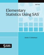
What happens if you reduce the sample size even further, so that each sample contains only 10 values? What happens if you reduce the sample size to 5 values?
Figure 6.2 shows the results of reducing the sample size. All of the histograms have the same scale to make comparing them easier.
The averages for the larger sample sizes are more closely grouped around the true population mean of $4850. The range of values for the larger sample sizes is smaller than it is for the smaller sample sizes. The following table lists the 2.5% and 97.5% values for these samples. This range encompasses about 95% of the averages.

The population with the smallest sample size of 5 values has the widest range that includes 95% of the averages. This matches the results in Figure 6.2, where the histogram for the sample size of 5 has the widest range of values.
This example shows how larger sample sizes produce more precise estimates. An estimate from a larger sample size is more likely to be closer to the true population mean.
However, collecting sample data requires time and often costs money. At some point, increasing the sample size does not provide practical value. For example, increasing the sample size to 10,000 for the salary example is unlikely to provide an estimate where the increased precision is worth the time and effort to collect such a large sample.
Effect of Population Variability
This section continues with the salary example and explores how population variability affects the estimates from a sample. Recall that one measure of population variability is the standard deviation—σ. As the population standard deviation decreases, the sample average is a more precise estimate of the population mean.
Estimation with a Smaller Population Standard Deviation
Suppose that the true population standard deviation is $300, instead of $625. Note that you cannot change the population standard deviation the way you can change the sample size. The true population standard deviation is fixed, so you are now collecting samples from a different distribution of the population with a true population mean of $4850, and a true population standard deviation of $300. Suppose you collect 200 samples of size 10 from a population with a true standard deviation of $300. What happens to the histogram of sample averages?
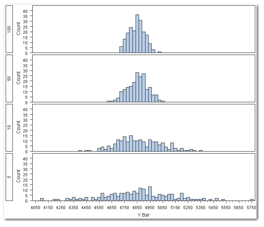
What if the true population standard deviation is even smaller, say, $150? Now the samples are from another distribution of the population with a true population standard deviation of $150. What happens if the true population standard deviation is even smaller, say, $75?
Figure 6.3 shows the results for smaller population standard deviations. All of the histograms have the same scale to make comparing them easier.
The averages for the populations with smaller standard deviations are more closely grouped around the true population mean of $4850. The range of values for the smaller standard deviations is smaller than it is for the larger standard deviations.
The following table lists the 2.5% and 97.5% values for these samples. This range encompasses about 95% of the averages.

The population with the largest standard deviation of 625 has the widest range that includes 95% of the averages. This matches the results in Figure 6.3, where the histogram for the population standard deviation of 625 has the widest range of values.
This example shows how samples from populations with smaller standard deviations produce more precise estimates. An estimate from a population with a smaller standard deviation is more likely to be closer to the true population mean.
The Distribution of Sample Averages
Figures 6.2 and 6.3 show how the sample size and the population standard deviation affect the estimate of the population mean. Look again at all of the histograms in Figures 6.2 and 6.3. Just as individual values in a sample have a distribution, so do the sample averages. This section discusses the distribution of sample averages.
The histogram of sample averages in Figure 6.1 is roughly bell-shaped. Normal distributions are bell-shaped. Combining these two facts, you conclude that sample averages are approximately normally distributed.
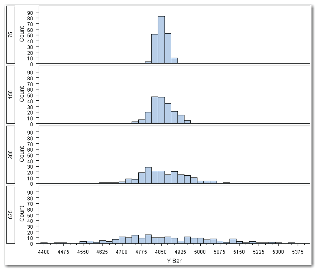
You might think that this initial conclusion is correct only because the samples are from a normal distribution (because salaries can conceivably be from a normal distribution). The fact is that your initial conclusion is correct even for populations that cannot conceivably be from a normal distribution. As an example, consider another type of distribution—the exponential distribution. One common use for this type of distribution is to estimate the time to failure. For example, think about laptops, which typically have a 3-hour battery. Suppose you measure the time to failure for the battery for 100 laptops. Figure 6.4 shows a histogram of this sample.
Now, suppose you measure the time to failure for the battery in 30 laptops, and repeat this process 200 times. (Note that this description simplifies the experiment. In a real experiment, you would need to control the types of laptops, the types of batteries, and so on. However, for this example, assume that the experiment has been run correctly.) Figure 6.5 shows a histogram of the averages.

The distribution is roughly bell-shaped. This leads you to initially conclude that the sample averages are approximately normally distributed. The fact that sample averages from non-normal distributions are approximately normally distributed is one of the most important foundations of statistical theory.
The Central Limit Theorem is a formal mathematical theorem that supports your initial conclusion. Essentially, the Central Limit Theorem says the following:
If you have a simple random sample of n observations from a population with mean µ and standard deviation σ
and if n is large
then the sample average ![]() is approximately normally distributed with mean µ and standard deviation
is approximately normally distributed with mean µ and standard deviation ![]() .
.
The list below shows two important practical implications of the Central Limit Theorem:
- Even if the sample values are not normally distributed, the sample average is approximately normally distributed.
- Because the sample average is approximately normally distributed, you can use the Empirical Rule to summarize the distribution of sample averages.
How Big Is Large?
The description of the Central Limit Theorem says “and if n is large.” How big is large? The answer depends on how non-normal the population is. For moderately non-normal populations, sample averages based on as few as 5 observations (n=5) tend to be approximately normally distributed. But, if the population is highly skewed or has heavy tails (for example, it contains a lot of extremely large or extremely small values), then a much larger sample size is needed for the sample average to be approximately normally distributed. For practical purposes, samples with more than 5 observations are usually collected.
One reason for collecting larger samples is because larger sample sizes produce more precise estimates of the population mean. See Figure 6.2 for an illustration.
A second reason for collecting larger samples is to increase the chance that the sample is a representative sample. Small samples, even if they are random, are less likely to be representative of the entire population. For example, an opinion poll that is a random sample of 150 people might not be as representative of the entire population as an opinion poll that is a random sample of 1000 people. (Note that stratified random sampling, mentioned in Chapter 5, can enable you to use a smaller sample. Collecting larger random samples might not always be the best way to sample.)
The Standard Error of the Mean
The Central Limit Theorem says that sample averages are approximately normally distributed. The mean of the normal distribution of sample averages is µ, which is also the population mean. The standard deviation of the distribution of sample averages is ![]() , where σ is the standard deviation of the population. The standard deviation of the distribution of sample averages is called the standard error of the mean.
, where σ is the standard deviation of the population. The standard deviation of the distribution of sample averages is called the standard error of the mean.
The Empirical Rule and the Central Limit Theorem
One of the practical implications of the Central Limit Theorem is that you can use the Empirical Rule to summarize the distribution of sample averages.
- About 68% of the sample averages are between µ–
 and µ+.
 - About 95% of the sample averages are between µ–2 and µ+2.
- More than 99% of the sample averages are between µ–3 and µ+3
From now on, this book uses “between µ±2![]() ” to mean “between µ–2
” to mean “between µ–2![]() and µ+2
and µ+2![]() ”
”
The following table uses the second statement of the Empirical Rule to calculate the range of values that includes 95% of the sample averages. The last column of the table shows the 2.5% and 97.5% percentiles for the monthly salary data (which includes 95% of the sample averages). With different data, the range for the data would change. Because the Empirical Rule is based on the population mean, the population standard deviation, and the sample size, the range for the Empirical Rule stays the same. For this data, the ranges for the actual data are close to the ranges for the Empirical Rule. Sometimes the ranges are higher, and sometimes lower, but generally the ranges are close.

With many sample averages, you can get a good estimate of the population mean by looking at the distribution of sample averages. You can use the distribution of sample averages to determine how close your estimate should be to the true population mean. However, typically, you have only one sample average. This one sample average gives a point estimate of the population mean, but a point estimate might not be close to the true population mean (as you have seen in the previous examples in this chapter). What if you want to get an estimate with upper and lower limits around it? To do this, get a confidence interval for the mean. The next section describes how.
Getting Confidence Intervals for the Mean
A confidence interval for the mean gives an interval estimate for the population mean. This interval estimate places upper and lower limits around a point estimate for the mean. The examples in this chapter show how the sample average estimates the population mean, and how the sample size and population standard deviation affect the precision of the estimate. The chapter also explains how the Central Limit Theorem and the Empirical Rule can be used to summarize the distribution of sample averages. A confidence interval uses all of these ideas.
A 95% confidence interval is an interval that is very likely to contain the true population mean (µ). Specifically, if you collect a large number of samples, and then calculate a confidence interval for each sample, 95% of the confidence intervals would contain the true population mean (µ), and 5% would not. Unfortunately, with only one sample, you don’t know whether the confidence interval you calculate is in the 95%, or in the 5%. However, you can consider your interval to be one of many intervals. And, any one of these many intervals has a 95% chance of containing the true population mean. Thus, the term “confidence interval” indicates your degree of belief or confidence that the interval contains the true population mean. The term “confidence interval” is often abbreviated as CI.
Recall the 95% bound on estimates suggested by the Central Limit Theorem and the Empirical Rule. A conceptual bound to use in a 95% confidence interval can be determined with the formula ![]() because this is the bound that contains 95% of the distribution of sample averages. However, in most real-life applications, the population standard deviation (σ) is unknown. A natural substitution is to use the sample standard deviation (s) to replace the population standard deviation (σ) in the formula. After you make this replacement, the conceptual bound formula is
because this is the bound that contains 95% of the distribution of sample averages. However, in most real-life applications, the population standard deviation (σ) is unknown. A natural substitution is to use the sample standard deviation (s) to replace the population standard deviation (σ) in the formula. After you make this replacement, the conceptual bound formula is ![]() . However, if you replace σ with s in the formula, the number 2 in the formula is not correct.
. However, if you replace σ with s in the formula, the number 2 in the formula is not correct.
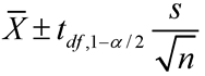
The normal distribution is completely defined by the population mean (µ) and the population standard deviation (σ). If you replace σ with s, the use of the normal distribution (and, thus, the Empirical Rule) is not exactly correct. A t distribution should be used instead of the normal distribution. A t distribution is very similar to the normal distribution, and allows you to adjust for different sample sizes. Now, the conceptual bound formula becomes ![]() . The value of t (or the t-value) is based on the sample size and level of confidence you choose. The formula for a confidence interval for the mean is as follows:
. The value of t (or the t-value) is based on the sample size and level of confidence you choose. The formula for a confidence interval for the mean is as follows:

![]()
is the sample average.
![]()
is the t-value for a given df and α. The df is one less than the sample size (df=n-1), and is called the degrees of freedom for the t-value. As n gets large, the t-value approaches the value for a normal distribution. The confidence level for the interval is 1- α. For a 95% confidence level, α =0.05. Calculating a 95% confidence interval for a data set with 12 observations requires t11,0.975 (which is 2.201). When finding the t-value, divide α by 2 before subtracting it from 1.
s
is the sample standard deviation.
n
is the sample size.
You can use PROC MEANS to get a confidence interval for the mean. As discussed in Chapter 4, you can use statistics-keywords to request statistics that the procedure does not automatically display in the output.
The data in Table 6.1 consists of interest rates for mortgages from several banks. Because mortgage rates differ based on discount points, the size of the loan, the length and type of loan, and whether an origination fee is charged, the data consists of interest rates for the same type of loan. Specifically, the interest rates in the data set are for a 30-year fixed-rate loan for $295,000, with no points and a 1% origination fee. Also, because interest rates change quickly (sometimes, even daily), all of the information was collected on the same day. The actual bank names are not used.

This data is available in the rates data set in the sample data for the book. In SAS, the following code calculates confidence intervals:
data rates;
input mortrate @@;
label mortrate='Mortgage Rate';
datalines;
5.750 5.750 5.500 5.750 5.500 5.750 5.750 5.750 5.625
5.750 5.875 5.625 5.875 5.625 5.750 5.750 5.750 5.875
5.750 5.875 5.625 5.750 5.750 5.500 5.750 5.500 5.625
5.750 5.500 5.625
;
run;
proc means data=rates n mean stddev clm maxdec=3;
var mortrate;
title 'Summary of Mortgage Rate Data';
run;
The PROC MEANS statement uses statistics-keywords discussed in Chapter 4 (N, MEAN, and STDDEV), and uses a new keyword, CLM, for the confidence limits for the mean.
The MAXDEC= option controls the number of decimal places that are displayed. This option can be useful in reports or presentations.
Figure 6.6 shows the output. The confidence limits are displayed under the headings Lower 95% CL for Mean and Upper 95% CL for Mean.
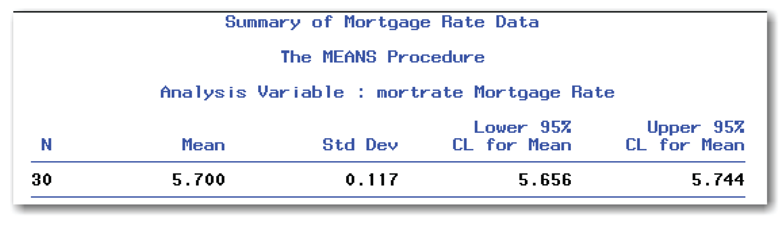
Confidence intervals are often shown enclosed in parentheses, with the lower and upper confidence limits separated by a comma—for example, (5.656, 5.744). For this data, you can conclude with 95% confidence that the true mean mortgage rate for this type of loan is between 5.656% and 5.744%.
PROC MEANS automatically creates a 95% confidence interval. As discussed in Chapter 5 regarding significance levels, your situation determines the confidence level you choose.
Using the rates data, suppose you want a 90% confidence interval. In SAS, the following code calculates this confidence interval:
proc means data=rates n mean stddev clm alpha=0.10;
var mortrate;
title 'Summary of Mortgage Rate Data with 90% CI';
run;
The ALPHA= option specifies the confidence level for the confidence interval. For a 90% confidence interval, α=0.10.
Figure 6.7 shows the output. The confidence limits are displayed under the headings Lower 90% CL for Mean and Upper 90% CL for Mean. Figure 6.7 shows how PROC MEANS automatically displays statistics when the MAXDEC= option is omitted.

The 90% confidence interval for the mortgage rate is (5.66, 5.74). When you decrease the confidence level from 95% to 90%, the confidence interval is narrower. To clarify, compare the two confidence intervals in the table below:
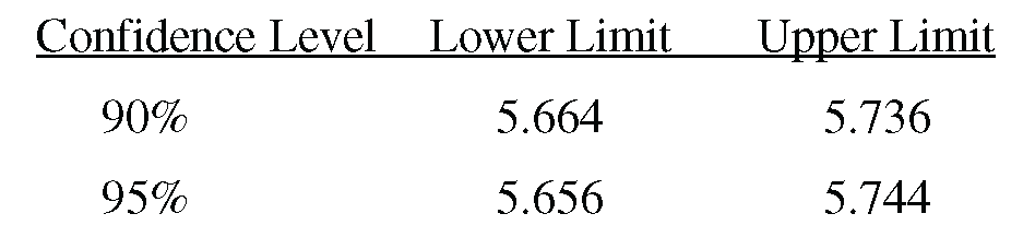
The 95% confidence interval is wider than the 90% confidence interval. When you decrease the alpha level from 0.10 to 0.05, the confidence interval with the lower alpha level is wider.
The general form of the statements to add confidence intervals is shown below:
PROC MEANS DATA=data-set-name N MEAN STDDEV CLM
MAXDEC=number ALPHA=value;
VAR variables;
data-set-name is the name of a SAS data set, and variables lists one or more variables in the data set.
The MAXDEC= option controls the number of decimal places to display.
The ALPHA= option must be between 0 and 1. The reason is because confidence intervals must be between 0% and 100%. The automatic value is ALPHA=0.05, which produces 95% confidence intervals.
You can use the MAXDEC= option and ALPHA= option together. You can use other statistics-keywords in the PROC MEANS statement. See Chapter 4 for examples.
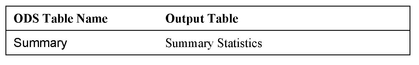
PROC MEANS includes the confidence interval in the table of summary statistics. Table 6.2 identifies the ODS table name.
- Larger sample sizes produce more precise estimates of the population mean than smaller sample sizes.
- Samples from populations with small standard deviations produce more precise estimates of the population mean than samples from populations with large standard deviations.
- The Central Limit Theorem says that for large samples, the sample average is approximately normally distributed, even if the sample values are not normally distributed.
- To calculate confidence intervals for the mean when the population standard deviation is unknown, use the following formula:
![]() is the sample average, n is the sample size, and s is the sample standard deviation. The value of
is the sample average, n is the sample size, and s is the sample standard deviation. The value of ![]() is a t-value that is based on the sample size and the confidence level. The degrees of freedom (df) is one less than the sample size (df=n-1), and 1- α is the confidence level for the confidence interval. For a 95% confidence interval for a data set with 12 observations, the t needed is t11,0.975.
is a t-value that is based on the sample size and the confidence level. The degrees of freedom (df) is one less than the sample size (df=n-1), and 1- α is the confidence level for the confidence interval. For a 95% confidence interval for a data set with 12 observations, the t needed is t11,0.975.
To create confidence intervals using PROC MEANS, change the number of decimal places displayed, and change the confidence level
PROC MEANS DATA=data-set-name N MEAN STD CLM
MAXDEC=number ALPHA=value;
VAR variables;
data-set-name
is the name of a SAS data set.
variables
lists one or more variables in the data set.
MAXDEC=
specifies the number of places to print after the decimal point.
ALPHA=
must be between 0 and 1. The reason is because confidence intervals must be between 0% and 100%. The automatic value is ALPHA=0.05, which produces 95% confidence intervals.
You can use the MAXDEC= option and ALPHA= options together. You can also use other statistics-keywords in the PROC MEANS statement. See Chapter 4 for examples.
The program that produced output for the simulations is not shown. The program below produces the output shown in this chapter for the rates data set.
data rates;
input mortrate @@;
label mortrate='Mortgage Rate';
datalines;
5.750 5.750 5.500 5.750 5.500 5.750 5.750 5.750 5.625
5.750 5.875 5.625 5.875 5.625 5.750 5.750 5.750 5.875
5.750 5.875 5.625 5.750 5.750 5.500 5.750 5.500 5.625
5.750 5.500 5.625
;
run;
proc means data=rates n mean stddev clm maxdec=3;
var mortrate;
title 'Summary of Mortgage Rate Data';
run;
proc means data=rates n mean stddev clm alpha=0.10;
var mortrate;
title 'Summary of Mortgage Rate Data with 90% CI';
run;