Chapter 10 Understanding Correlation and Regression

Can SAT scores be used to predict college grade point averages? How does the age of a house affect its selling price? Is heart rate affected by the amount of blood cholesterol? How much of an increase in sales results from a specific increase in advertising expenditures?

These questions involve looking at two continuous variables, and investigating whether the variables are related. As one variable increases, does the other variable increase, decrease, or stay the same? Because both variables contain quantitative measurements, comparing groups is not appropriate. This chapter discusses the following topics:

• summarizing continuous variables using scatter plots and statistics.
• using correlation coefficients to describe the strength of the linear relationship between two continuous variables.
• performing least squares regression analysis to develop equations that describe how one variable is related to another variable. Sections discuss fitting straight lines, fitting curves, and fitting an equation with more than two continuous variables.
• enhancing the regression analysis by adding confidence curves.

The methods in this chapter are appropriate for continuous variables. Regression analyses that handle other types of variables exist, but they are outside the scope of this book. See Appendix 1, “Further Reading,” for suggested references.

Chapters 10 and 11 discuss the activities of regression analysis and regression diagnostics. Fitting a regression model and performing diagnostics are intertwined. In regression, you first fit a model. Then, you perform diagnostics to assess how well the model fits. You repeat this process until you find a suitable model. This chapter focuses on fitting models. Chapter 11 focuses on performing diagnostics.

Summarizing Multiple Continuous Variables

Creating Scatter Plots

Creating a Scatter Plot Matrix

Using Summary Statistics to Check Data for Errors

Reviewing PROC CORR Syntax for Summarizing Variables

Calculating Correlation Coefficients

Understanding Correlation Coefficients

Understanding Tests for Correlation Coefficients

Working with Missing Values

Reviewing PROC CORR Syntax for Correlations

Cautions about Correlations

Questions Not Answered by Correlation

Performing Straight-Line Regression

Understanding Least Squares Regression

Explaining Regression Equations

Assumptions for Least Squares Regression

Steps in Fitting a Straight Line

Fitting a Straight Line with PROC REG

Finding the Equation for the Fitted Straight Line

Understanding the Parameter Estimates Table

Understanding the Fit Statistics Table

Understanding the Analysis of Variance Table

Understanding Other Items in the Results

Using PROC REG Interactively

Printing Predicted Values and Limits

Plotting Predicted Values and Limits

Summarizing Straight-Line Regression

Fitting Curves

Understanding Polynomial Regression

Fitting Curves with PROC REG

Understanding Results for Fitting a Curve

Printing Predicted Values and Limits

Plotting Predicted Values and Limits

Summarizing Polynomial Regression

Regression for Multiple Independent Variables

Understanding Multiple Regression

Fitting Multiple Regression Models in SAS

Understanding Results for Multiple Regression

Printing Predicted Values and Limits

Summarizing Multiple Regression

Summary

Key Ideas

Syntax

Example

Special Topic: Line Printer Plots

Summarizing Multiple Continuous Variables

This section discusses methods for summarizing continuous variables. Chapter 4 described how to use summary statistics (such as the mean) and graphs (such as histograms and box plots) for a continuous variable. Use these graphs and statistics to check the data for errors before performing any statistical analyses.

For continuous variables, a scatter plot with one variable on the y-axis and another variable on the x-axis shows the possible relationship between the continuous variables. Scatter plots provide another way to check the data for errors.

Suppose a homeowner was interested in the effect that using the air conditioner had on the electric bill. The homeowner recorded the number of hours the air conditioner was used for 21 days, and the number of times the dryer was used each day. The homeowner also monitored the electric meter for these 21 days, and computed the amount of electricity used each day in kilowatt-hours.[1] Table 10.1 displays the data.

This data is available in the kilowatt data set in the sample data for the book. To create the data set in SAS, submit the following:

data kilowatt;

input kwh ac dryer @@;

datalines;

35 1.5 1 63 4.5 2 66 5.0 2 17 2.0 0 94 8.5 3 79 6.0 3

93 13.5 1 66 8.0 1 94 12.5 1 82 7.5 2 78 6.5 3 65 8.0 1

77 7.5 2 75 8.0 2 62 7.5 1 85 12.0 1 43 6.0 0 57 2.5 3

33 5.0 0 65 7.5 1 33 6.0 0

;

run;

Creating Scatter Plots

SAS provides several ways to create scatter plots. PROC CORR produces both scatter plots and statistical reports. When you begin to summarize several continuous variables, using PROC CORR can be more efficient because you can perform all of the summary tasks with this one procedure.

ods graphics on;

ods select ScatterPlot;

proc corr data=kilowatt

plots=scatter(noinset ellipse=none);

var ac kwh;

run;

ods graphics off;

The ODS statement specifies that PROC CORR print only the scatter plot. The ODS GRAPHICS statements activate and deactivate the graphics for the procedure. See “Using ODS Statistical Graphics” in the next section.

In the PROC CORR statement, PLOTS=SCATTER specifies a scatter plot. NOINSET suppresses an automatic summary that shows the number of observations and the correlation coefficient (discussed later in this chapter). ELLIPSE=NONE suppresses the automatic prediction ellipse. The first variable in the VAR statement identifies the variable for the x-axis, and the second variable identifies the variable for the y-axis. When you use this combination of options, PROC CORR prints a simple scatter plot of the two variables. Figure 10.1 shows the results.

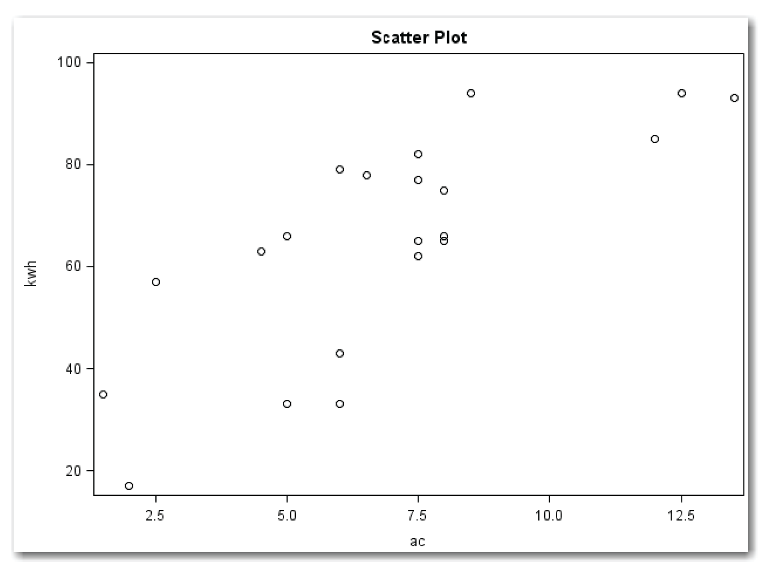
This simple scatter plot shows that higher values of kwh tend to occur with higher values of ac. However, the relationship is not perfect because some days have higher ac values with lower kwh values. This difference is because of other factors (such as how hot it was or how many other appliances were used) that affect the amount of electricity that was used on a given day.

Using ODS Statistical Graphics

As described in Chapter 4, you can use the ODS statement to control the output that is printed by a procedure. SAS includes ODS Statistical Graphics for some procedures.[2] ODS Statistical Graphics is a versatile and complex system that provides many features. This section discusses the basics.

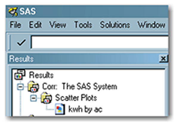
The simplest way to use ODS Statistical Graphics is to use the automatic approach of including the graphs in SAS output. The key difference between ODS Statistical Graphics and plain ODS is that SAS displays the graphs in a separate window (when using ODS Statistical Graphics) rather than in the Graphics window (when using ODS). Figure 10.2 shows an example of how ODS Statistical Graphics output is displayed in the Results window when you are in the windowing environment mode. ODS Statistical Graphics created the graph labeled kwh by ac. For convenience, the rest of Chapter 10 and all of Chapter 11 use the term “ODS graphics” to refer to ODS Statistical Graphics.

To use ODS graphics, you activate the feature before a procedure, and you deactivate the feature afterward. Look at the code before Figure 10.1. The first statement activates ODS graphics for PROC CORR, and the last statement deactivates ODS graphics.

The general form of the statements to activate and then deactivate ODS graphics in a SAS procedure is shown below:

ODS GRAPHICS ON;

ODS GRAPHICS OFF;

Creating a Scatter Plot Matrix

A simple scatter plot of two variables can be useful. When you have more than two variables, a scatter plot matrix can help you understand the possible relationships between the variables. A scatter plot matrix shows all possible simple scatter plots for all combinations of two variables:

ods graphics on;

ods select MatrixPlot;

proc corr data=kilowatt

plots=matrix(histogram nvar=all);

var ac dryer kwh;

run;

ods graphics off;

The ODS statement specifies that PROC CORR print only the scatter plot matrix. The VAR statement lists all of the variables that you want to plot.

In the PROC CORR statement, PLOTS=MATRIX specifies a scatter plot matrix. HISTOGRAM adds a histogram for each variable along the diagonal of the matrix.[3] NVAR=ALL includes all variables in the VAR statement in the scatter plot matrix. SAS automatically uses NVAR=5 for a 5x5 scatter plot matrix. For the kilowatt data, this option is not needed, but it is shown in the example to help you with your data.

Figure 10.3 shows the results.

The scatter plot matrix shows all possible two-way scatter plots for the three variables. (For your data, the matrix will show all possible two-way scatter plots for the variables you choose.) The center diagonal automatically identifies the variables. When you use the HISTOGRAM option, the center diagonal displays a histogram for each variable. Figure 10.4 helps decode the structure of the scatter plot matrix.

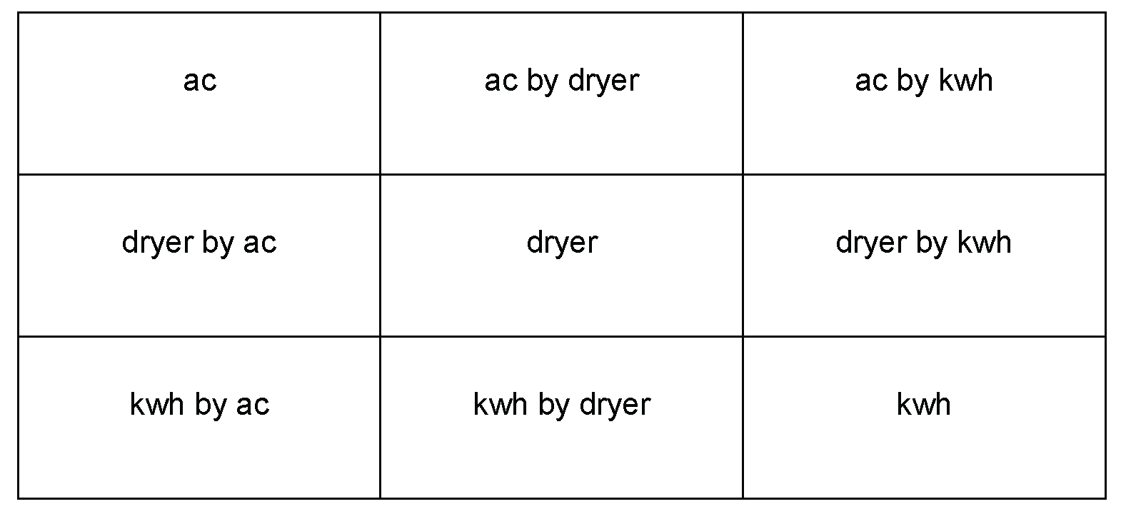
The ac by kwh scatter plot in the upper right corner shows ac on the y-axis and kwh on the x-axis. The lower left corner shows the mirror image of this scatter plot, with kwh on the y-axis and ac on the x-axis. kwh is the response variable, or the variable whose values are impacted by the other variables. Typically, scatter plots show the response variable on the vertical y-axis, and the other variables on the x-axis. PROC CORR shows the full scatter plot matrix, and you choose which scatter plot to use.

Look at the lower left corner of Figure 10.3. This is the same scatter plot as the simple scatter plot in Figure 10.1. This plot shows that higher values of kwh tend to occur with higher values of ac.

The kwh by dryer scatter plot shows that higher values of kwh tend to occur with higher values of dryer. By just looking at the scatter plot, this increasing relationship does not appear to be as strong as the increasing relationship between kwh and ac.

The histograms along the diagonal of Figure 10.3 help show the distribution of values for each variable. You can see that dryer has only a few values, and that kwh appears to be skewed to the right.

Figure 10.3 illustrates another benefit of a scatter plot matrix. It can highlight potential errors in the data by showing potential outlier points in two directions. For the kilowatt data, all of the data points are valid. Another example of a benefit of the scatter plot matrix is with blood pressure readings. A value of 95 for systolic blood pressure (the higher number of the two numbers) for a person is reasonable. Similarly, a value of 95 for diastolic blood pressure (the lower number of the two numbers) for a person is reasonable. However, a value of 95/95 for systolic/diastolic is not reasonable. Checking the two variables one at a time (with PROC UNIVARIATE, for example) would not highlight the value of 95/95 for systolic/diastolic as an issue. However, the scatter plot matrix would highlight this value as a potential outlier point that should be investigated.

Using Summary Statistics to Check Data for Errors

As a final task of summarizing continuous variables, think about checking the data for errors. The scatter plot matrix is an effective way to find potential outlier points. Chapter 4 discussed using box plots to find outlier points, and it recommended checking the minimum and maximum values to confirm that they seem reasonable. You could use PROC UNIVARIATE to produce a report of summary statistics for each variable, but using PROC CORR can be more efficient:

ods select SimpleStats;

proc corr data=kilowatt;

var ac dryer kwh;

title 'Summary Statistics for KILOWATT Data Set';

run;

The ODS statement specifies that PROC CORR print only the simple summary statistics table. The VAR statement lists all of the variables that you want to summarize.

Figure 10.5 shows the results.

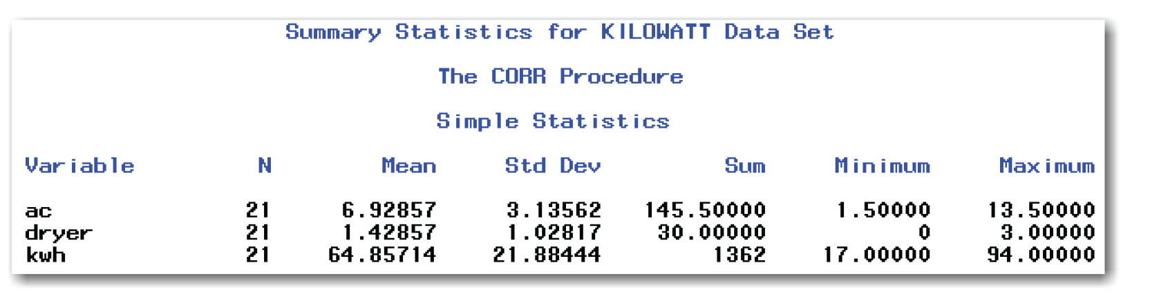
SAS identifies the variables under the Variable heading in the Simple Statistics table. See Chapter 4 for definitions of the other statistics in the other columns.

SAS uses all available values to calculate these statistics. Suppose the homeowner forgot to collect dryer information on one day, resulting in only 20 values for the dryer variable. The Simple Statistics table would show N as 20 for dryer, and N as 21 for the other two variables.

Reviewing PROC CORR Syntax for Summarizing Variables

The general form of the statements to summarize and plot variables using PROC CORR is shown below:

ODS GRAPHICS ON;

PROC CORR DATA=data-set-name options;

VAR variables;

ODS GRAPHICS OFF;

data-set-name is the name of a SAS data set, and variables are the variables that you want to plot or summarize. If you omit the variables from the VAR statement, then the procedure uses all numeric variables.

The PROC CORR statement options can be:

PLOTS=SCATTER(scatter-options)

creates a simple scatter plot for the variables.

SAS uses the first variable in the VAR statement for the x-axis, and the second variable for the y-axis. If you use more than two variables, then SAS creates a scatter plot for each pair of variables. Thescatter-options can be one or more of the following:

NOINSET

suppresses an automatic summary that shows the number of observations and the correlation coefficient.

ELLIPSE=NONE

suppresses the automatic prediction ellipse.

If you use scatter-options, then the parentheses are required.

And, the PROC CORR statement options can be:

PLOTS=MATRIX(matrix-options)

creates a scatter plot matrix for the variables.

The matrix-options can be one or more of the following:

HISTOGRAM

adds a histogram for each variable along the diagonal of the matrix.[4]

NVAR=ALL

includes all variables in the VAR statement in the scatter plot matrix. SAS automatically uses NVAR=5, so, if your data has fewer than 5 variables, you can omit this option.

If you use matrix-options, then the parentheses are required.

You can use both PLOTS=SCATTER and PLOTS=MATRIX in the same PROC CORR statement.

You can use the ODS statement to specify the output tables to print. (See “Special Topic: Using ODS to Control Output Tables” at the end of Chapter 4 for more detail.) Table 10.2 identifies the output tables for PROC CORR summary statistics and plots.

Calculating Correlation Coefficients

PROC CORR automatically produces correlation coefficients. In the previous sections, ODS statements have suppressed the correlation coefficients.

Understanding Correlation Coefficients

PROC CORR automatically produces Pearson correlation coefficients. Statistical texts represent the Pearson correlation coefficient with the letter “r.” Values of r range from -1.0 to +1.0.

With positive correlation coefficients, the values of the two variables increase together. With negative correlation coefficients, the values of one variable increase, while the values of the other variable decrease. Values near 0 imply that the two variables do not have a linear relationship.

A correlation coefficient of 1 (r=+1) corresponds to a plot of points that fall exactly on an upward-sloping straight line. A correlation coefficient of (r=-1) corresponds to a plot of points that fall exactly on a downward-sloping straight line. (Neither of these straight lines necessarily has a slope of 1.) The correlation of a variable with itself is always +1. Otherwise, values of +1 or -1 usually don’t occur in real situations because plots of real data don’t fall exactly on straight lines.

In reality, values of r are between -1 and +1. Relatively large positive values of r, such as 0.7, correspond to a plot of points that have an upward trend. Relatively large negative values of r, such as -0.7, correspond to a plot of points that have a downward trend.

What defines the terms “near 0” or “relatively large”? How do you know whether the correlation coefficient measures a strong or weak relationship between two continuous variables? SAS provides these answers in the Pearson Correlation Coefficients table:

proc corr data=kilowatt;

var ac dryer kwh;

title 'Correlations for KILOWATT Data Set';

run;

The PROC CORR and VAR statements are the same as the statements used to produce simple statistics. The example above does not use an ODS statement, so the results contain all automatic reports from SAS.

Figure 10.6 shows the results.

Figure 10.6 contains three tables. The Variables Information table lists the variables. The Simple Statistics table shows summary statistics, as described in the previous section. The Pearson Correlation Coefficients table shows the correlation coefficients and the results of statistical tests.

The Pearson Correlation Coefficients table displays the information for the variables in a matrix. This matrix has the same structure as the scatter plot matrix. See Figure 10.4 to help understand the structure. The heading for the table identifies the top number as the correlation coefficient, and the bottom number as a p-value. (See the next section, “Understanding Tests for Correlation Coefficients,” for an explanation of the bottom number.) Because the data values are all nonmissing, the heading for the table also identifies the number of observations.

Figure 10.6 shows that the relationship between ac and kwh has a positive correlation of 0.76528. Figure 10.6 shows that there is a weaker positive relationship between dryer and kwh with the correlation coefficient of 0.59839. Figure 10.6 shows a very weak negative relationship between ac and dryer with the correlation coefficient of –0.02880. These results confirm the visual understanding from the scatter plot matrix.

The correlation coefficients along the diagonal of the matrix are 1.00000 because the correlation of a variable with itself is always +1.

Understanding Tests for Correlation Coefficients

The Pearson Correlation Coefficients table displays a p-value as the bottom number in most cells of the matrix. The table does not display a p-value for cells along the diagonal because the correlation of a variable with itself is always +1 and the test is not relevant.

The heading for the table identifies the test as Prob > |r| under H0: Rho=0. The true unknown population correlation coefficient is called Rho. (Chapter 5 discusses how population parameters are typically denoted by Greek letters.) For this test, the null hypothesis is that the correlation coefficient is 0. The alternative hypothesis is that the correlation coefficient is different from 0. This test provides answers to the questions of whether a correlation coefficient is relatively large or near 0.

Suppose you choose a 5% significance level. This level implies a 5% chance of concluding that the correlation coefficient is different from 0 when, in fact, it is not. This decision gives a reference probability of 0.05.

For the kilowatt data, focus on the two correlation coefficients involving kwh. Both of these correlation coefficients are significantly different from 0. The ac and kwh test has a p-value of <.0001. The dryer and kwh test has a p-value of 0.0042. These results confirm the visual understanding from the scatter plot matrix.

In addition, the results for ac and dryer confirm the visual understanding from the scatter plot matrix. With a p-value of 0.9014, you conclude that there is not a linear relationship between these two variables.

In general, if the p-value is less than the significance level, then reject the null hypothesis, and conclude that the correlation coefficient is significantly different from 0. If the p-value is greater than the significance level, then you fail to reject the null hypothesis. You conclude that there is not enough evidence that the correlation coefficient is significantly different from 0.

Working with Missing Values

The kilowatt data has no missing values, so PROC CORR simply prints the number of observations in the heading for the Pearson Correlation Coefficients table.

For data sets with missing values, PROC CORR automatically uses as many observations as possible. Suppose the homeowner did not collect dryer information on the first day. The value for dryer would be missing for the first observation. (Suppose this data is the kilowatt2 data set.) The statements below cause the automatic behavior to occur:

proc corr data=kilowatt2;

var ac dryer kwh;

title 'Automatic Behavior with Missing Values for KILOWATT2';

run;

Figure 10.7 shows the results.

Figure 10.7 indicates the missing value for dryer in the Simple Statistics table with an N of 20. Figure 10.7 shows a third value in each cell in the Pearson Correlation Coefficients table. The heading for the table identifies this third value as Number of Observations. Compare the values in the cells. Any cell that involves dryer also involves only 20 observations because of the missing value.

In situations with several variables and missing values, you might want to use only the observations where all variables have data values. The NOMISS option in the PROC CORR statement limits analyses to the observations where all variables are nonmissing. The statements below use this option.

proc corr data=kilowatt2 nomiss;

var ac dryer kwh;

title 'NOMISS Option for KILOWATT2';

run;

Figure 10.8 shows the results.

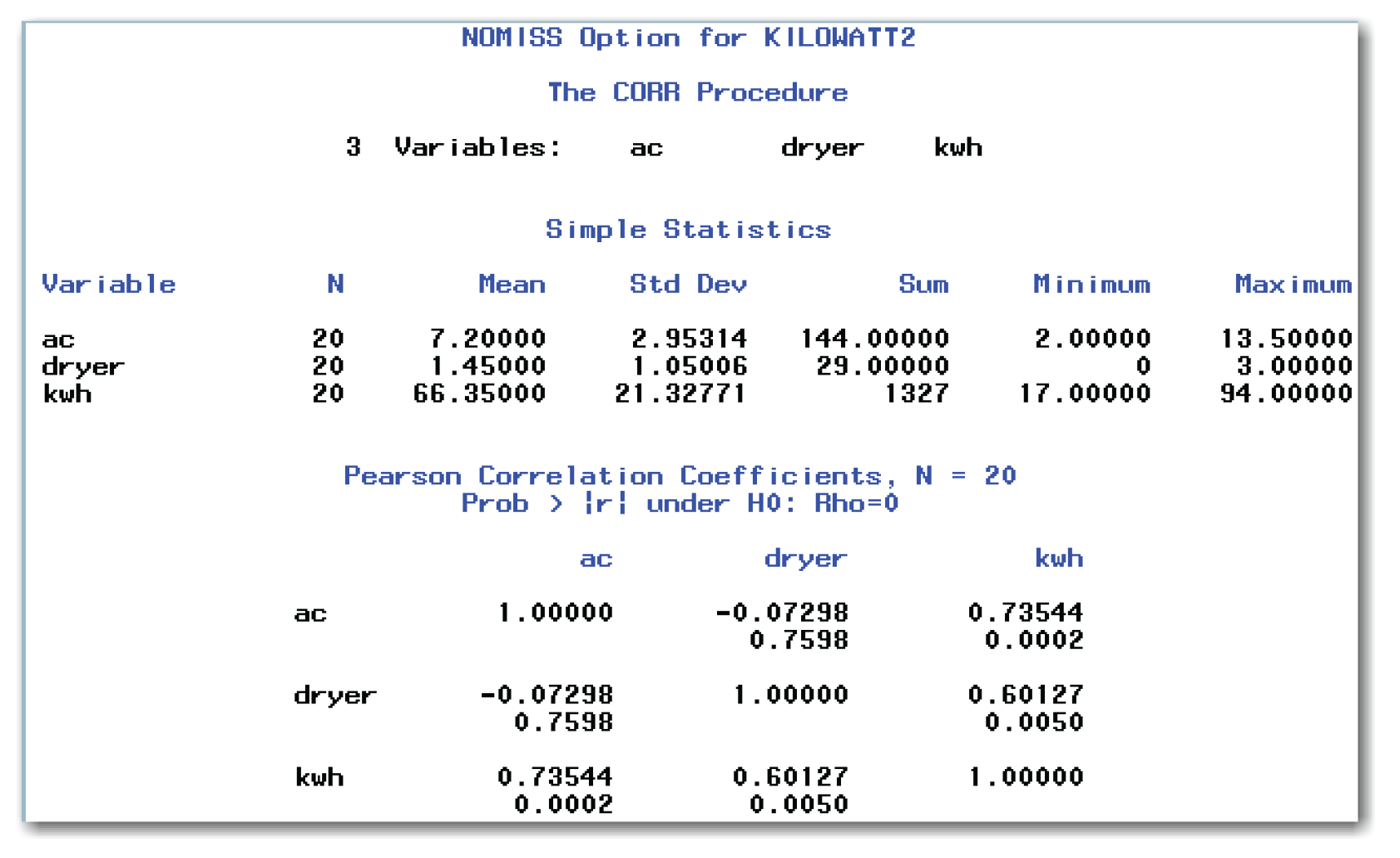
Compare the results in Figure 10.7 and 10.8. Figure 10.8 shows an N of 20 for all variables. Figure 10.8 does not show the third value in each cell in the Pearson Correlation Coefficients table. Instead, the heading for the table identifies the number of observations as 20 for all correlations.

If your data has missing values, you might want to consider the NOMISS option. However, with many missing values, you might exclude a large number of observations, and you might receive misleading results. In this situation, consult a statistician because another analysis might be more appropriate for your data.

Reviewing PROC CORR Syntax for Correlations

The general form of the statements to create correlation coefficients and tests using PROC CORR is shown below:

PROC CORR DATA=data-set-name options;

VAR variables;

The PROC CORR statement options can be as defined earlier and can also be:

NOMISS

excludes observations with missing values.

If you omit the variables from the VAR statement, then the procedure uses all numeric variables. Specify at least two variables for the output to be meaningful because the correlation of a variable with itself is always +1.

Other items in italic were defined earlier.

You can use the ODS statement to specify the output tables to print. (See “Special Topic: Using ODS to Control Output Tables” at the end of Chapter 4 for more detail.) Table 10.4 identifies the output tables for PROC CORR.

Cautions about Correlations

There are two important cautions to remember when interpreting correlations.

First, correlation is not the same as causation. When two variables are highly correlated, it does not necessarily imply that one variable causes the other. In some cases, there might be an underlying causal relationship, but you don’t know this information from the correlation coefficient. In other cases, the relationship might be caused by a different variable. For example, consider a store owner who notices a high positive correlation between the sales of ice scrapers and hot coffee. Coffee sales don’t cause ice scraper sales, and the reverse is not true, either. Perhaps the sales of both of these items are caused by weather—drivers purchasing more hot coffee and more ice scrapers on cold, snowy days. Proving cause-and-effect relationships is much more difficult than showing a high correlation.

Second, “shopping for significance” in a large group of correlations is not a good idea. Researchers sometimes make the mistake of measuring many variables, finding the correlations between all possible pairs of variables, and choosing the significant correlations to make conclusions. Recall the interpretation of a significance level, and you see the mistake: If a researcher performs 100 correlations, and tests their significance at the 0.05 significance level, then about 5 significant correlations will be found by chance alone.

Questions Not Answered by Correlation

From the value of r in Figure 10.6, you conclude that as the use of the air conditioner increases, so do the kilowatt-hours (kwh) that are consumed. This is not a surprise. Here are some other important questions:

• How many kilowatt-hours are consumed for each hour of using the air conditioner?
• What is a prediction of the kilowatt-hour consumption for a specific day when the air conditioner is used for a specified number of hours?
• What is an estimate of the average kilowatt-hour consumption on days when the air conditioner is used for a specified number of hours?
• What are the confidence limits for the predicted kilowatt-hour consumption?

A regression analysis of the data answers these questions. The next sections discuss fitting a straight line with regression analysis, fitting a curve, and regression analysis with multiple x variables.

Performing Straight-Line Regression

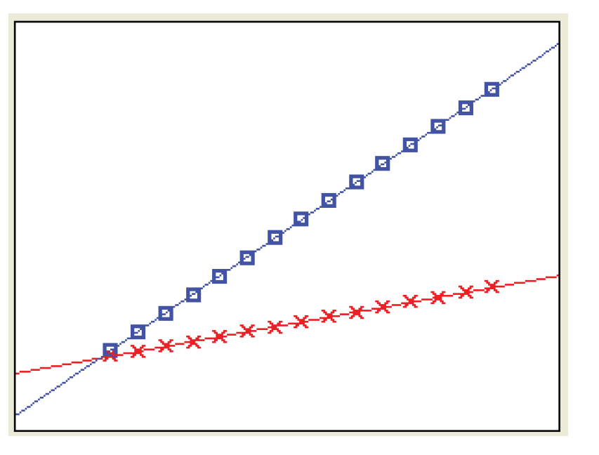
A correlation coefficient indicates that a linear relationship exists, and the p-value evaluates the strength of this linear relationship. However, a correlation coefficient does not fully describe the relationship between the two variables. Figure 10.9 shows a plot for two different y variables against the same x variable. The correlation coefficient between y and x is 1.0 in both cases. All of the points for each y variable fall exactly on a straight line. However, the relationships between y and x are quite different for the two y variables.

Look again at the kwh by ac scatter plot in Figure 10.1. You could draw a straight line through the data points. In a room of people, each person would draw a slightly different straight line. Which straight line is “best”? The next three sections discuss statistical methods and assumptions for fitting the “best” straight line to data.

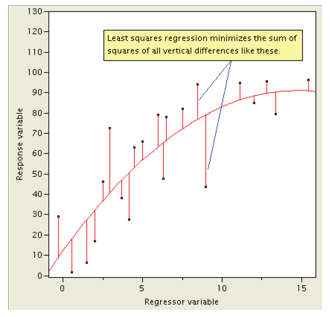
Understanding Least Squares Regression

Least squares regression fits a straight line through the data points that minimizes the vertical differences between all of the points and the straight line. Figure 10.10 shows this approach. For each data point, calculate the vertical difference between the data point and the straight line. Then, square the difference. This gives points above and below the line the same importance (squared differences are all positive). Finally, sum the squared differences. The “best” straight line is the line that minimizes the sum of squared differences, which is the basis of the name “least squares regression.”

Explaining Regression Equations

The regression equation summarizes a straight-line relationship between two variables:

y = β0 + β1 x + ε

The y variable is the dependent variable or the response variable. The x variable is the independent variable or the regressor variable. The equation says that the dependent variable y is a straight-line function of x, with an intercept β0 and a slope β1. The intercept is the value of the y-axis when x=0. The slope is the amount of vertical increase for a one-unit horizontal increase. In algebra, this is called “the rise over the run.” For the kilowatt data, the slope estimates the average number of kilowatt-hours for running the air conditioner for one hour.

Because a given x value does not always lead to the same y value, the data has random variation. The equation uses ε to denote the random variation. For the kilowatt data, the homeowner knows how long the air conditioner was used each day. But, other appliances and lights consume electricity in varying amounts from day to day. This variation is the “error” in the model equation. For straight-line regression, the “error” includes both the random variation in the data and other potential variables (such as dryer) that are not included in the model equation.

Statisticians use this equation when they have the entire population of values for x and y. In that case, the regression equation describes the entire population. In reality, you usually collect just a sample, and then use the sample data to estimate the straight line for the entire population. In this case, you use the following equation:

ŷ = b0 + b1 x

b0 and b1 are the estimates of β0 and β1, respectively. The value b0 gives the predicted value of y when x is 0. The value b1 gives the increase in the y value that results from a one-unit increase in x. The values of b0 and b1 are called parameter estimates because they estimate the unknown population parameters β0 and β1, respectively. The value ŷ indicates the predicted value of the response variable from the equation.

Assumptions for Least Squares Regression

Like all analyses, least squares regression requires some assumptions. Here they are:

• The data values are measurements. Both the x and y variables are continuous.

For the kilowatt data, this assumption seems reasonable.

• Observations are independent. The values from one pair of x-y observations are not related to the values from another pair. To check the assumption, think about your data and whether this assumption seems reasonable. This is not a step where using SAS will answer this question.

For the kilowatt data, the observations are independent because the measurements for one day are not related to the measurements for other days.

• Observations are a random sample from the population. You want to make conclusions about a larger population, not about just the sample. To check the assumption, think about your data and whether this assumption seems reasonable. This is not a step where using SAS will answer this question.

For the kilowatt data, you want to make conclusions about kwh and ac use in general, not for just the 21 days in the data set. Assuming that the days in the study are a random sample of all possible days seems reasonable.

• The values of x variables are known without error. To check the assumption, think about your data and whether this assumption seems reasonable. This is not a step where using SAS will answer this question.

For the kilowatt data, assuming that the homeowner accurately measured the number of hours that the air conditioner was used seems reasonable.

• The errors in the data are normally distributed with a mean of 0 and a variance of σ2. However, the regression equation has meaning even if the assumption does not seem reasonable. This assumption is needed for hypothesis tests and confidence intervals. (Chapter 11 discusses this assumption. For now, assume that it seems reasonable.)

Steps in Fitting a Straight Line

The steps for performing the regression analysis are basically the same as the steps for comparing groups:

1. Create a SAS data set.

2. Check the data set for errors.

3. Choose the significance level.

4. Check the assumptions.

5. Perform the test.

6. Make conclusions from the results.

For the kilowatt data, steps 1, 2, and 4 are done. For step 3, choose a 5% significance level, which requires a p-value less than 0.05 to conclude that the regression coefficients are different from 0. This level implies a 5% chance of concluding that the regression coefficients are different from 0 when, in fact, they are not.

Fitting a Straight Line with PROC REG

As with scatter plots, SAS provides more than one way to fit a straight line to the data. In fact, SAS includes more than 25 procedures that perform regression. This book focuses on PROC REG, which performs linear regression and includes diagnostic statistics and plots. If the topics in this chapter do not fit your situation, then check the SAS documentation. SAS very likely provides a procedure that meets your needs. To fit a straight line to kwh and ac in SAS:

proc reg data=kilowatt;

model kwh=ac;

plot kwh*ac / nostat cline=red;

title 'Straight-line Regression for KILOWATT Data';

run;

When performing regression, PROC REQ requires the MODEL statement. The MODEL statement above identifies kwh as the response (y) variable, and ac as the independent (x) variable. The PLOT statement is not required. Above, the PLOT statement produces a scatter plot with the fitted straight line.[5] NOSTAT suppresses several statistics that automatically appear to the right of the scatter plot. CLINE=RED specifies that the regression line is red.

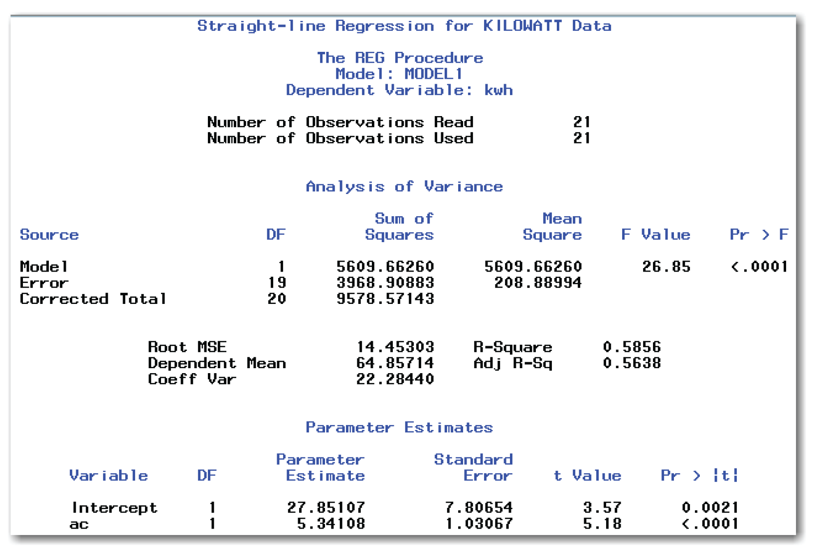
Figure 10.11 shows the scatter plot. Figure 10.12 shows the printed results.

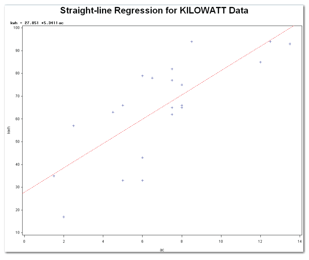
The scatter plot shows the fitted regression equation above the plot on the left.

The printed tables provide details for the regression analysis. The next five sections discuss these tables.

Finding the Equation for the Fitted Straight Line

First, answer the research question, “What is the relationship between the two variables?” Figure 10.11 shows the red fitted straight line in the scatter plot. Just above the scatter plot, on the left, SAS shows the equation for the fitted line:

kwh = 27.85 + 5.34*ac

This equation rounds the SAS parameter estimates to two decimal places.

The fitted line has an intercept value of 27.85. When the homeowner does not use the air conditioner at all, the fitted line predicts that 27.85 kilowatt-hours will be used that day.

The fitted line has a slope of 5.34. The homeowner uses 5.34 kilowatt-hours of electricity when the air conditioner runs for 1 hour. If the homeowner uses the air conditioner for 8 hours, the fitted line predicts that 42.72 (5.34*8) kilowatt-hours of electricity will be used.

For this entire day, the fitted line predicts the following:

kilowatt-hours = 27.85 + (5.34*8)

= 27.85 + 42.72

= 70.57

Correlation coefficients could not provide an answer to the question of how many kilowatt-hours are consumed for one hour’s use of the air conditioner. The slope of the regression line gives the answer of 5.34 kilowatt-hours. (Because a kilowatt is 1000 watts, the air conditioner uses 5340 watts per hour. This is more kilowatt-hours than would be consumed by fifty-three 100-watt light bulbs.)

Another goal was to predict the kilowatt-hours that are consumed when using the air conditioner for a specified number of hours. Again, the regression line gives the answer, as shown in the equation for using the air conditioner for 8 hours. (See “Printing Predicted Values and Limits” and “Plotting Predicted Values and Limits” for more detail.)

Figure 10.12 shows the estimates for the intercept and slope in the Parameter Estimates table.

As with correlation coefficients, a natural question about the intercept and slope is whether they are significantly different from 0. The next section explains how to find the answer to this question.

Understanding the Parameter Estimates Table

Figure 10.12 shows the Parameter Estimates table, which answers the question about the significance of the estimates for the intercept and the slope. SAS tests the null hypothesis that the parameter estimate is 0. The alternative hypothesis is that the parameter estimate is different from 0.

Look under the heading Pr > |t| in Figure 10.12. The p-values for the intercept and the slope are 0.0021 and <.0001, respectively. Because these values are less than the significance level of 0.05, you reject the null hypothesis, and you conclude that the intercept and slope are significantly different from 0.

The statistical results make sense because the slope indicates that increasing the number of hours that the air conditioner is used produces an increase in the kilowatt-hours for that day. The intercept is significantly different from 0, which indicates that even if the homeowner does not use the air conditioner, some kilowatt-hours are consumed that day.

In general, to interpret SAS results, look at the p-values under the heading Pr > |t|. If the p-value is less than your significance level, reject the null hypotheses that the parameter estimate is 0. If the p-value is greater, you fail to reject the null hypothesis.

The list below describes items in the Parameter Estimates table:

Variable

identifies the parameter. SAS identifies the intercept as Intercept, and the slope of the line by the regressor variable (ac in this example).

DF

is the degrees of freedom for the parameter estimate. This should equal 1 for each parameter.

Parameter Estimate

lists the parameter estimate.

Standard Error

is the standard error of the estimate. It measures how much the parameter estimates would vary from one collection of data to the another collection of data.

t Value

gives the t-value for testing the hypothesis. SAS calculates the t-value as the parameter estimate divided by its standard error.

For example, the t-value for the slope is 5.341/1.031, which is 5.18.

Understanding the Fit Statistics Table

Think about testing the parameter estimates. If neither the intercept nor the slope is significantly different from 0, then the straight line does not fit the data very well. The Fit Statistics table provides statistical tools to assess the fit.

Find the value for R-Square in Figure 10.12. This statistic is the proportion of total variation in the y variable due to the x variables in the model. R-Square ranges from 0 to 1 with higher values indicating better-fitting models. For the kilowatt data, R-Square is 0.5856. Statisticians often express this statistic as a percentage, saying that the model explains about 59% of the variation in the data (for this example).

The Fit Statistics table provides other statistics. The Dependent Mean is the average for the y variable. Compare the Dependent Mean value in Figure 10.12 with the Mean value for kwh in Figure 10.5, and confirm that they are the same. See the SAS documentation for explanations of the other statistics in this table.

Understanding the Analysis of Variance Table

The Analysis of Variance table looks similar to tables in Chapter 9. For regression analysis, statisticians use this table to help assess whether the overall model explains a significant amount of the variation in the data. The table augments conclusions from the R-Square statistic. Statisticians typically evaluate the overall model before examining the details for individual terms in the model.

When performing regression, the null hypothesis for the Analysis of Variance table is that the variation in the y variable is not explained by the variation in the x variable (for straight-line regression). The alternative hypothesis is that the variation in the y variable is explained by the variation in the x variable. Statisticians often refer to these hypotheses as testing whether the model is significant or not.

Find the value for Pr > F in Figure 10.12. This is the p-value for testing the hypothesis. Compare this p-value with the significance level. For the kilowatt data, the p-value of <.0001 is less than 0.05. You conclude that the variation in ac explains a significant amount of the variation in kwh.

In general, to interpret SAS results, look at the p-value under the heading Pr > F. If the p-value is less than your significance level, reject the null hypotheses that the variation in the y variable is not explained by the variation in the x variable. If the p-value is greater, you fail to reject the null hypothesis.

Chapter 9 describes the other information in the Analysis of Variance table. In Chapter 9, see “Understanding Results” in “Performing a One-Way ANOVA.”

Figure 10.12 shows the DF for Model as 1. When fitting a straight line with a single independent variable, the DF for Model will always be 1. In general, the degrees of freedom for the model is one less than the number of parameters estimated by the model. When fitting a straight line, PROC REG estimates two parameters—the intercept and the slope—so the model has 1 degree of freedom.

Figure 10.12 shows that the Sum of Squares for Model and Error add to be the Corrected Total. Here is the equation:

9578.57 = 5609.66 + 3968.91

Statisticians usually abbreviate sum of squares as SS. They describe the sum of squares with this equation:

Total SS = Model SS + Error SS

This is a basic and important equation in regression analysis. Regression partitions total variation into variation due to the variables in the model, and variation due to error.

The model cannot typically explain all of the variation in the data. For example, Table 10.1 shows three observations with ac equal to 8 and with kwh values of 66, 65, and 75. Because the three different kwh values occurred on days with the same value of 8 for ac, the straight-line regression model cannot explain the variation in these data points. This variation must be due to error (or due to factors other than the use of the air conditioner).

Understanding Other Items in the Results

PROC REG uses headings and the Number of Observations table to identify the data used in the regression.

The heading contains two lines labeled Model and Dependent Variable. The dependent variable is the measurement variable on the left side of the equation in the MODEL statement. PROC REG assigns a label to each MODEL statement. PROC REG automatically uses MODEL1 for the model in the first MODEL statement, MODEL2 for the model in the second MODEL statement, and so on. This book uses the automatic labels.

The Number of Observations table lists the number of observations read from the data set, and the number of observations used in the regression. Because the kilowatt data does not have missing values, PROC REG uses all observations in the analysis. For your data, PROC REG uses all observations with nonmissing values for the variables in the regression.

Using PROC REG Interactively

PROC REG is an interactive procedure. If you use line mode or the windowing environment mode, you can perform an analysis of variance, and then perform other tasks without rerunning the regression. Type the PROC REG and MODEL statements, and add a RUN statement to see the results. Then, you can add other statements and a second RUN statement to perform other tasks. The following statements produce the output shown in Figures 10.11 and 10.12:

proc reg data=kilowatt;

model kwh=ac;

title 'Straight-line Regression for KILOWATT Data';

run;

plot kwh*ac / nostat cline=red;

run;

quit;

When you use these statements, the second RUN statement does not end PROC REG because the procedure is waiting to receive additional statements. The QUIT statement ends PROC REG. The form of the QUIT statement is simply the word QUIT followed by a semicolon.

Although you can end the procedure by starting another DATA or PROC step, you might receive an error. If you use an ODS statement before the next PROC step, and the table you specify in the ODS statement is not available in PROC REG (which is running interactively), SAS prints an error in the log and does not create output. To avoid this situation, use the QUIT statement.

Printing Predicted Values and Limits

The section “Finding the Equation for the Fitted Straight Line” showed how to predict how many kilowatt-hours are consumed when the air conditioner is used for 8 hours on a given day. You can manually use the equation to predict other values, or you can let SAS provide the predictions. You can also add two types of confidence limits.

Defining Prediction Limits

Remember that correlations could not provide confidence limits for an individual predicted kilowatt-hour consumption. Table 10.1 shows three days in the data where the homeowner used the air conditioner for 8 hours (ac=8). The regression equation predicts the same kilowatt-hours for these three days. But, the actual kilowatt-hours for these days range from 65 to 75.

Suppose you want to put confidence limits on the predicted value of 70.57 (calculated in the section “Finding the Equation for the Fitted Straight Line”). Just as confidence limits for the mean provide an interval estimate for the unknown population mean, confidence limits for a predicted value provide an interval estimate for the unknown future value. These confidence limits on individual values need to account for possible error in the fitted regression line. They need to account for variation in the y variable for observations that have the same value of the x variable. Statisticians often refer to confidence limits on individual values as prediction limits.

Defining Confidence Limits for the Mean

Suppose you want to estimate the average kilowatt-hours that are consumed on all days when the air conditioner is used for a given number of hours. This task is essentially the same task as estimating the average kilowatt-hours that are consumed on a given day. In other words, to predict a single future value or to estimate the mean response for a given value of the independent variable, you use the same value from the regression equation.

For example, suppose you want to estimate the mean kilowatt-hour consumption for all days when the air conditioner is used for 8 hours. To get an estimate for each day, insert the value ac=8 into the fitted regression equation. Because ac is the same for all of these days, the equation produces the same predicted value for kwh. It makes sense to use this predicted value as an estimate of the mean kilowatt-hours consumed for all of these days.

Next, you can add confidence limits on the average kilowatt-hours that are consumed when the air conditioner is used for 8 hours. These confidence limits will differ from the prediction limits.

Because the mean is a population parameter, the mean value for all of the days with a given value for ac does not change. Because the mean does not vary and the actual values do vary, it makes sense that a confidence interval for the mean would be smaller than the confidence interval for a single predicted value. With a single predicted value, you need to account for the variation between actual values, as well as for any error in the fitted regression line. With the mean, you need to account for only the error in the fitted regression line.

Using PROC REG to Print Predicted Values and Limits

Because PROC REG is an interactive procedure, you can print predicted values, prediction limits, and confidence limits for the mean using one of two approaches. You can provide options in the MODEL statement, or you can use the PRINT statement. For both approaches, use the same option names for the statistics requested. For both approaches, the optional ID statement adds a column that identifies the observations. PROC REG requires that the ID statement appear before the first RUN statement. The two PROC REG activities below produce the same output.

proc reg data=kilowatt;

id ac;

model kwh=ac / p clm cli;

run;

quit;

proc reg data=kilowatt;

id ac;

model kwh=ac;

run;

print p clm cli;

run;

quit;

The first PROC REG activity uses options in the MODEL statement and produces the results in Figures 10.12 and 10.13. The second PROC REG activity uses the PRINT statement and options, and produces the results in Figures 10.12 and 10.13. With the second approach, you can add results to the PROC REG output without re-running the model.

Both PROC REG activities use the same options. The P option requests predicted values, CLI requests prediction limits, and CLM requests confidence limits for the mean.

Figure 10.13 shows the same heading as Figure 10.12. It also shows the Output Statistics table.

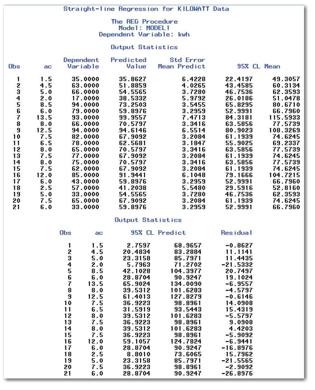
The list below describes items in the Output Statistics table:

Obs

identifies the observations by observation number.

ac

identifies the observations by the value of ac. For your data, the heading and values will reflect the variable you use in the ID statement.

Dependent Variable

are actual values of the response variable kwh.

Predicted Value

are predicted values of the response variable kwh.

Observations 8, 12, and 14 have a predicted value of 70.5797. These are the three observations with ac=8, so the predicted values are the same. The Predicted Value differs slightly from what was computed in “Finding the Equation for the Fitted Straight Line” because the equation in the book rounds off the parameter estimates.

Std Error Mean Predict

is the standard error of the predicted value. It is used in calculating confidence limits for the mean.

95% CL Mean

the left column gives the lower confidence limit for the mean, and the right column gives the upper confidence limit for the mean. For observation 8 with ac=8, the 95% confidence limits are 63.59 and 77.57. This means that you can be 95% confident that the mean kilowatt-hour consumption on a day with ac=8 will be somewhere between 63.59 and 77.57.

95% CL Predict

the left column gives the lower prediction limit, and the right column gives the upper prediction limit. For observation 8 with ac=8, the 95% prediction limits are 39.53 and 101.63. This means that you can be 95% confident that the kilowatt-hour consumption on a day with ac=8 will be somewhere between 39.53 and 101.62.

Residual

gives the residuals, which are the differences between actual and predicted values. Residuals are calculated by subtracting the predicted value from the actual value. For the first observation, the residual is 35.0-35.86=-0.86. You might find it helpful to think of the residual as the amount by which the fitted regression line “missed” the actual data point. Chapter 11 discusses using residuals for regression diagnostics.

Compare the prediction limits and the confidence limits for the mean for an observation in Figure 10.13. The confidence limits for the mean are narrower than the prediction limits. Especially for larger data sets, plotting the limits can be more helpful than looking at the table.

Plotting Predicted Values and Limits

PROC REG provides multiple ways to plot. You can use ODS graphics, similar to the approach used with PROC CORR earlier in the chapter. You can use the PLOT statement to produce high-resolution graphs, and you can also use the PLOT statement to produce line printer plots. This section discusses using ODS graphics and the PLOT statement for high-resolution graphs. See “Special Topic: Line Printer Plots” at the end of the chapter for information about line printer plots.

Using ODS Graphics

The statements below use ODS graphics to create a plot that shows the data, fitted line, prediction limits, and confidence limits for the mean:

ods graphics on;

proc reg data=kilowatt plots(only)=fit(stats=none);

model kwh=ac;

title 'Straight-line Regression for KILOWATT Data';

run;

quit;

ods graphics off;

The first ODS GRAPHICS statement activates ODS graphics, as described earlier in this chapter. The PLOTS= option in the PROC REG statement uses several additional plotting options.[6] ONLY limits the plots to plots specified after the equal sign. When you use ODS graphics, PROC REG automatically produces several plots. (Chapter 11 discusses the other plots, which are useful for regression diagnostics.) FIT requests a plot with the fitted line, prediction limits, and confidence limits for the mean. STATS=NONE suppresses a table of statistics that automatically appears on the right side of the plot. Figure 10.14 shows the plot.

Figure 10.14 shows the data points as circles, and the fitted regression line as the thick, dark blue, solid line. The confidence limits for the mean are shown by the inner, blue-shaded area. The confidence limits for individual predicted values are shown by the outer, dashed, blue lines. SAS provides the legend below the plot as a helpful reminder.

You can use additional plotting options with ODS graphics to suppress the prediction limits, confidence limits, or both. The statements below use NOCLI to suppress the prediction limits shown in Figure 10.14:

ods graphics on;

proc reg data=kilowatt plots(only)=fit(nocli stats=none);

model kwh=ac;

run;

quit;

ods graphics off;

The statements below use NOCLM to suppress the confidence limits for the mean shown in Figure 10.14:

ods graphics on;

proc reg data=kilowatt plots(only)=fit(noclm stats=none);

model kwh=ac;

run;

quit;

ods graphics off;

The statements below use NOLIMITS to suppress both the prediction limits and the confidence limits for the mean shown in Figure 10.14:

ods graphics on;

proc reg data=kilowatt plots(only)=fit(nolimits stats=none);

model kwh=ac;

run;

quit;

ods graphics off;

Using Traditional Graphics with the PLOT Statement

When you use the PLOT statement to produce high-resolution graphs, SAS documentation refers to these graphs as “traditional graphics.” To create these graphs, you must have SAS/GRAPH software licensed. Figure 10.11 shows a scatter plot and fitted regression line created by the PLOT statement. By adding plotting options, the plot can include limits. When you add prediction limits and confidence limits for the mean, SAS automatically chooses a different color for each line. You can use SYMBOL statements to specify the same color for both the upper and lower prediction limits, and to specify another color for both the upper and lower confidence limits for the mean. This approach produces better graphs for presentations or reports.

The statements below assume that you have fit a straight line to the data, and that you are using PROC REG interactively. (If this is not the case, then add the PROC REG and MODEL statements.)

symbol1 color=blue;

symbol2 color=red line=1;

symbol3 color=green line=2;

symbol4 color=green line=2;

symbol5 color=purple line=3;

symbol6 color=purple line=3;

plot kwh*ac / pred conf nostat;

run;

quit;

The SYMBOL1 statement controls the color of the data points. The SYMBOL2 statement controls the color and appearance of the fitted line. The next two statements control the color and appearance of the confidence limits for the mean. The last two SYMBOL statements control the color and appearance of the prediction limits. SAS provides more than 45 line types, and SAS Help shows examples of each type. In general, the COLOR= option identifies the color, and the LINE= option specifies the line type.

In the PLOT statement, the NOSTAT option suppresses an automatic table of statistics as discussed earlier. The PRED option requests prediction limits, and the CONF option requests confidence limits for the mean. You can specify only one of these two options if you want. For example, you can use only the PRED option to create a plot with the fitted line and prediction limits.

Figure 10.15 shows the results.

Figure 10.15 shows the data points as plus signs. The lines have the colors specified in the SYMBOL statements.

Summarizing Straight-Line Regression

Straight-line regression uses least squares to fit a line through a set of data points. Predicted values for the y variable for a given x value are computed by inserting the value of x into the equation for the fitted line. Prediction limits account for the error in fitting the regression line, and account for the variation between values for a given x value. Confidence limits on the mean account for the error in fitting the regression line because the mean does not change. Plots of the observed values, fitted regression line, prediction limits, and confidence limits on the mean are useful in summarizing the regression.

Because this chapter uses PROC REG for fitting lines, curves, and regression with multiple variables, the summary for the general form of the procedure appears only in the “Syntax” section at the end of the chapter. Similarly, the list of ODS tables for PROC REG appears only in the “Summary” section.

After fitting a regression line, your next step is to perform regression diagnostics. The diagnostic tools help you decide whether the regression equation is adequate, or whether you need to add more terms to the equation. Perhaps another variable needs to be added, or a curve fits the data better than a straight line. Chapter 11 discusses a set of basic tools for regression diagnostics.

The next section discusses fitting curves.

Fitting Curves

Understanding Polynomial Regression

For the kilowatt data, a straight line described the relationship between air conditioner use and kilowatt-hours. In other cases, though, the relationship between two variables is not represented well by a straight line. Sometimes, a curve does a better job of representing the relationship. A quadratic polynomial has the following equation:

ŷ = b0 + b1 x + b2x2

With least squares regression, b0, b1, and b2 are estimates of unknown population parameters. The squared term (x2) is called the quadratic term when referring to the model.

If you could measure all of the values in the entire population, you would know the exact relationship between x and y. Because you can measure only values in a sample of the population, you estimate the relationship using regression. Least squares regression for curves minimizes the sum of squared differences between the points and the curve, as shown in Figure 10.16.

The assumptions for fitting a curve with least squares regression are the same as the assumptions for fitting a straight line. Similarly, the steps for fitting a curve are the same as the steps for fitting a straight line. As with fitting a straight line, PROC REG provides one way to fit a curve to data.

Fitting Curves with PROC REG

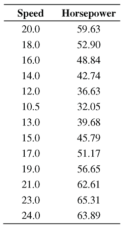
An engineer conducted an experiment to test the performance of an industrial engine. The experiment used a mixture of diesel fuel and gas derived from distilling organic materials. The engineer measured horsepower produced from the engine at several speeds, where speed is measured in hundreds of revolutions per minute (rpm x 100).[7] Table 10.2 shows the data.

The steps for fitting a curve are the following:

1. Create a SAS data set.

2. Check the data set for errors. Assume that you have performed this step and found no errors.

3. Choose the significance level. Choose a significance level of 0.05. This level implies a 5% chance of concluding that the regression coefficients are different from 0 when, in fact, they are not.

4. Check the assumptions.

5. Perform the analysis.

6. Make conclusions from the results.

This data is available in the engine data set in the sample data for the book. The statements below create the data set, and then use PROC CORR to create a scatter plot of the data. Figure 10.17 shows the scatter plot.

data engine;

input speed power @@;

speedsq=speed*speed;

datalines;

22.0 64.03 20.0 62.47 18.0 54.94 16.0 48.84 14.0 43.73

12.0 37.48 15.0 46.85 17.0 51.17 19.0 58.00 21.0 63.21

22.0 64.03 20.0 59.63 18.0 52.90 16.0 48.84 14.0 42.74

12.0 36.63 10.5 32.05 13.0 39.68 15.0 45.79 17.0 51.17

19.0 56.65 21.0 62.61 23.0 65.31 24.0 63.89

;

run;

ods graphics on;

ods select ScatterPlot;

proc corr data=engine plots=scatter(noinset ellipse=none);

var speed power;

title 'Scatterplot for ENGINE Data';

run;

ods graphics off;

The DATA step includes a program statement that creates the new variable SPEEDSQ. (See Chapter 7 for an introduction to program statements.) PROC REG requires individual names for the independent variables in the MODEL statement. As a result, PROC REG does not allow terms like SPEED*SPEED. The solution is to create a new variable for the quadratic term in the regression model.

Looking at the scatter plot in Figure 10.17, it seems like a straight line would not fit the data well. Power increases with Speed up to about 21, and then the data levels off or curves downward. Instead of fitting a straight line, fit a curve to the data.

Checking the Assumptions for Regression

Think about the assumptions:

• Both of the variables are continuous, and the data values are measurements.
• The observations are independent because the measurement for one observation of speed and power is unrelated to the measurement for another observation.
• The observations are a random sample from the population. Because this is an experiment, the engineer selected the levels of Speed in advance, selecting levels that made sense in the industrial environment where the engine would be used.
• The engineer can set the value for Speed precisely, so assume that the x variable is known without error.
• Chapter 11 discusses the assumption that the errors in the data are normally distributed. For now, assume that this assumption seems reasonable.

Performing the Analysis

To perform the analysis, submit the following:

proc reg data=engine;

id speed;

model power=speed speedsq / p cli clm;

title 'Fitting a Curve to the ENGINE Data';

run;

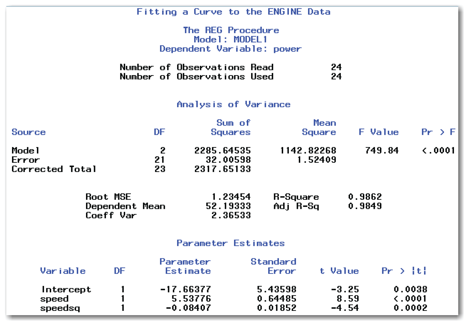
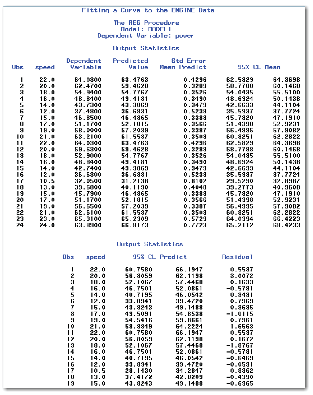
The statements above use the same statements and options for fitting a straight line. The key difference is the SPEEDSQ term in the MODEL statement. Because SPEEDSQ is calculated as speed2, this term is the quadratic term in the equation for fitting a curve. The ID statement identifies observations in the Output Statistics table. Figure 10.18 shows the results from the MODEL statement. Figure 10.19 shows the results of the options in the statement.

Figure 10.18 (for fitting a curve) shows the same SAS tables as Figure 10.12 (for fitting a straight line). Here are the key differences:

• The Parameter Estimates table now contains three parameters—Intercept, speed, and speedsq.
• The Analysis of Variance table shows a Model with 2 degrees of freedom. In general, the degrees of freedom for the model are one less than the number of parameters estimated by the model. When fitting a curve, PROC REG estimates three parameters, so the model has two degrees of freedom.

The next two sections focus on explaining the conclusions for the engine data.

Understanding Results for Fitting a Curve

First, answer the research question, “What is the relationship between the two variables?” Using the estimates from the Parameter Estimates table, here is the fitted equation:

power = -17.66 + 5.54*speed - 0.08*speed2

This equation rounds the SAS parameter estimates to two decimal places.

From the Parameter Estimates table, you conclude that all three coefficients are significantly different from 0. All three p-values are less than 0.05. At first, this might not make sense, because 0.08 seems close to 0. However, remember that the t Value divides the Parameter Estimate by Standard Error. Figure 10.18 shows a very small standard error for the coefficient of speedsq, and a correspondingly large t Value. This coefficient is multiplied by the speedsq value. Even though the coefficient is small, the impact of this term on the curve is important.

The Fit Statistics table shows R-Square is about 0.99, meaning that the fitted curve explains about 99% of the variation in the data. This is an excellent fit.

The Analysis of Variance table leads you to conclude that the fitted curve explains a significant amount of the variation in Power. The p-value for the F test is <.0001. Statisticians typically examine the overall test of the fitted model before reviewing the details of parameter estimates.

Printing Predicted Values and Limits

Just as when you fit a straight line, when you fit a curve, you can print confidence limits for the mean, and confidence limits on an individual predicted value. Figure 10.19 shows the first page of results from using the P, CLI, and CLM options in the MODEL statement. The second page shows the prediction limits and residuals for the last few observations in the data set.

Figure 10.19 for fitting a curve shows the same SAS tables as Figure 10.13. See the discussion after Figure 10.13 for an explanation of the columns in the output.

Changing the Alpha Level

SAS automatically creates 95% prediction limits and confidence limits for the mean. You can specify a different confidence level with the ALPHA= option in the PROC REG statement:

ods select OutputStatistics;

proc reg data=engine alpha=0.1;

model power=speed speedsq / p cli clm;

title '90% Limits for ENGINE Data';

run;

Because the regression fit for the model is the same as shown in Figure 10.18, the ODS statement limits the printed results to the Output Statistics table. The ALPHA= option specifies 90% confidence limits. Figure 10.20 shows the first page of the results.

Compare the results in Figures 10.19 and 10.20. The key difference is that Figure 10.20 shows 90% prediction limits and 90% confidence limits for the mean. When you use the ALPHA= option, PROC REG changes the alpha level for both types of limits.

You can also use the ALPHA= option when fitting a straight line or when performing multiple regression.

If you use the ALPHA= option and ODS graphics, then PROC REG applies the confidence level to the plots. For example, if you specify ALPHA=0.10, then ODS graphics display 90% prediction limits and 90% confidence limits for the mean.

Similarly, if you use the ALPHA= option and a PLOT statement, then PROC REG applies the confidence level to the plots.

Plotting Predicted Values and Limits

When fitting a curve, PROC REG has different choices for plotting. The ODS graphics FIT choice is not available. Also, the CONF and PRED options in the PLOT statement are not available. However, you can still use both ODS graphics and the PLOT statement to produce graphs. The next two sections show how.

Using ODS Graphics

The statements below use ODS graphics to create a plot that shows the data, fitted curve, prediction limits, and confidence limits for the mean.

ods graphics on;

ods select PredictionPlot;

proc reg data=engine alpha=0.10

plots(only)=predictions(x=speed unpack);

model power=speed speedsq;

run;

quit;

ods graphics off;

The first ODS GRAPHICS statement activates ODS graphics. The ODS statement limits the output to the plot. The PROC REG statement specifies ALPHA=0.10, so ODS graphics will create a plot with 90% confidence limits. The PLOTS option in the PROC REG statement uses several additional plotting options. ONLY limits the plots to plots specified after the equal sign. When you use ODS graphics, PROC REG automatically produces several plots. (Chapter 11 discusses the other plots, which are useful for regression diagnostics.) PREDICTIONS requests a plot with the fitted line, prediction limits, and confidence limits for the mean. Using x=speed specifies the x variable in the model. The PREDICTIONS option is appropriate only for models that have terms for a single variable. The models can be a straight line, curve, cubic model (with a linear, squared, and cubed term), and so on. The models cannot have more than a single x variable. PROC REG automatically produces two plots, and UNPACK separates these two plots. Figure 10.21 shows the first plot, which shows the fitted curve and limits. Chapter 11 discusses the second plot, which is useful for regression diagnostics.

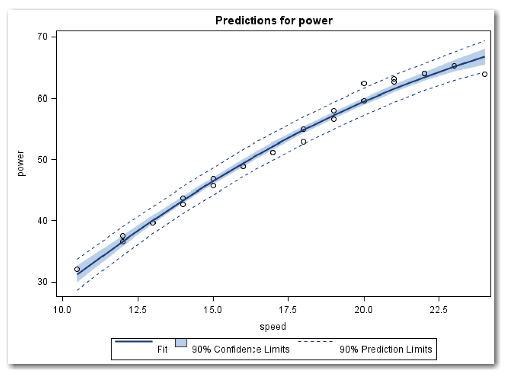
Figure 10.21 shows the data points as circles, and the fitted curve as the thick, dark blue, solid line. The confidence limits for the mean are shown by the inner, blue-shaded area. The confidence limits for individual predicted values are shown by the outer, dashed, blue lines. SAS provides the legend below the plot as a helpful reminder.

Figure 10.21 illustrates the narrow confidence curves for a model that fits very well. The curves for both the prediction limits and the confidence limits for the mean are very close to the fitted curve. Compare these limits for a model with an R-Square value of about 0.99 with the limits for a model that doesn’t fit as well in Figure 10.12 (with an R-Square value of about 0.59). This comparison illustrates a general principle: poorly fitting models generate wider confidence limits.

You can use additional plotting options with ODS graphics to suppress the prediction limits, confidence limits, or both. (See the discussion for using ODS graphics to plot a fitted line and limits earlier in this chapter.) You can use the NOCLI, NOCLM, and NOLIMITS options with PREDICTIONS. The statement below provides one example:

proc reg data=engine

plots(only)=predictions(x=speed noclm unpack);

To use NOCLI or NOLIMITS, replace NOCLM in the statement.

Using Traditional Graphics with the PLOT Statement

Although the CONF and PRED options in the PLOT statement are not available when fitting curves, you can use the PLOT statement and SYMBOL statements. The resulting plot does not display lines; it displays points instead. Here are the statements in SAS:[8]

symbol1 value=plus color=blue;

symbol2 value=dot color=red;

symbol3 value="I" color=purple;

symbol4 value="M" color=green;

symbol5 value="I" color=purple;

symbol6 value="M" color=green;

plot (power p. lcl. lclm. ucl. uclm.)*speed / overlay nostat;

run;

First, look at the PLOT statement. The statement identifies a single x variable—SPEED. The statement identifies several y variables, which are enclosed in parentheses. The first y variable is POWER, which plots the actual data values. The remaining y variables use statistical keywords and end with a dot (period). These keywords are defined in the table:

P.

predicted value

LCL.

lower prediction limit

LCLM.

lower confidence limit for the mean

UCL.

upper prediction limit

UCLM.

upper confidence limit for the mean

OVERLAY places all y*x plot requests on a single plot. NOSTAT suppresses several automatic statistics that appear to the right of the graph.

Next, look at the SYMBOL statements. SAS uses these statements based on the order of the y variables in the PLOT statement. For the example, SYMBOL1 controls the appearance of the actual data values, and SYMBOL2 controls the appearance of the predicted values. Because the prediction limits are the third and fifth y variables, the SYMBOL3 and SYMBOL5 statements control their appearance. Similarly, SYMBOL4 and SYMBOL6 control the appearance of the confidence limits for the mean.

The VALUE= option identifies the symbol used for the plotted point. SAS includes many automatic values. SYMBOL1 and SYMBOL2 use two of those automatic values. The remaining VALUE= options use text values. For your data, enter the single character enclosed in double quotation marks, as shown in the example.

Figure 10.22 shows the results.

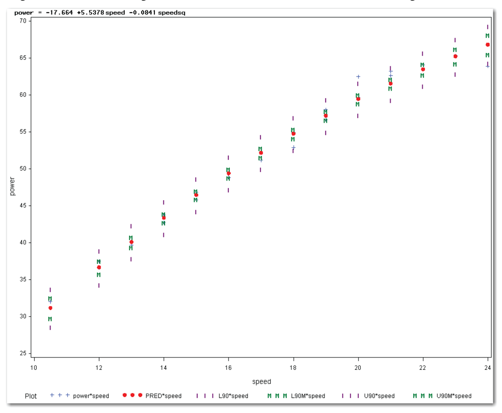
Data points in Figure 10.22 are difficult to see because either predicted values or points representing one of the limits overlay most of the data values.

Compare Figures 10.21 and 10.22. Figure 10.22 is more like a line printer plot. It does not show connected lines for the predicted values and limits. Instead, Figure 10.22 shows predicted values and limits for each x value in the data.

Summarizing Polynomial Regression

Fitting a curve to data involves a single dependent y variable, and a single x variable with a linear term and quadratic term. PROC REQ requires two separate variables for the linear term and quadratic term.

The same assumptions for fitting a straight line and the same analysis steps apply. Use PROC REG, and interpret the results in the same way. You can add confidence limits on the mean and on individual predicted values to the scatter plot. After you fit a curve, the next step is to perform diagnostics to check the fit of your model. Chapter 11 discusses a set of basic tools for regression diagnostics.

The next section discusses regression with more than one x variable.

Regression for Multiple Independent Variables

Understanding Multiple Regression

This chapter has discussed how to fit a straight line and a curve using regression. Both cases involved a single y variable and a single x variable. The curve included linear and quadratic (squared) terms for speed in the engine data, but the model included a single x variable.

Remember the homeowner-recorded dryer use for the kilowatt data? Suppose you want to add the dryer variable to the model. In this case, you are no longer fitting a straight line to the data because both ac and dryer are independent variables. Multiple regression is a regression model with multiple independent variables.

Multiple regression is difficult to picture in a simple scatter plot. For two independent variables, think of a three-dimensional picture. Figure 10.23 shows multiple regression, where the two independent variables are on the axes labeled X1 and X2, and the dependent variable is on the axis labeled Y. Multiple regression is the process of finding the best-fitting plane through the data points. Here, the term “best-fitting” is defined as the plane that minimizes the squared distances between all of the data points and the plane.

With two independent variables, here is the estimated regression equation:

ŷ = b0 + b1 x1 + b2x2

b0, b1, and b2 estimate the population parameters β0, β1, and β2. The two independent variables are x1 and x2.

The assumptions for multiple regression are the same as the assumptions for fitting a straight line. Similarly, the steps for multiple regression are the same as the steps for fitting a straight line.

Fitting Multiple Regression Models in SAS

For the kilowatt data, you use PROC REG with a different MODEL statement. Fit a multiple regression model with both ac and dryer as independent variables. You have already considered the assumptions for multiple regression because you considered these assumptions when fitting a straight line to the data. The only new assumption to consider for multiple regression is whether the homeowner measured dryer without error. Assume that the homeowner correctly recorded the number of times the dryer was used each day.

Also, assume that you want to continue to use an alpha level of 0.05.

proc reg data=kilowatt;

model kwh=ac dryer / p clm cli;

title 'Multiple Regression for KILOWATT Data';

run;

The program uses statements and options discussed earlier in this chapter. The key difference is that the MODEL statement now includes terms for the two independent variables—ac and dryer. Figure 10.24 shows the results.

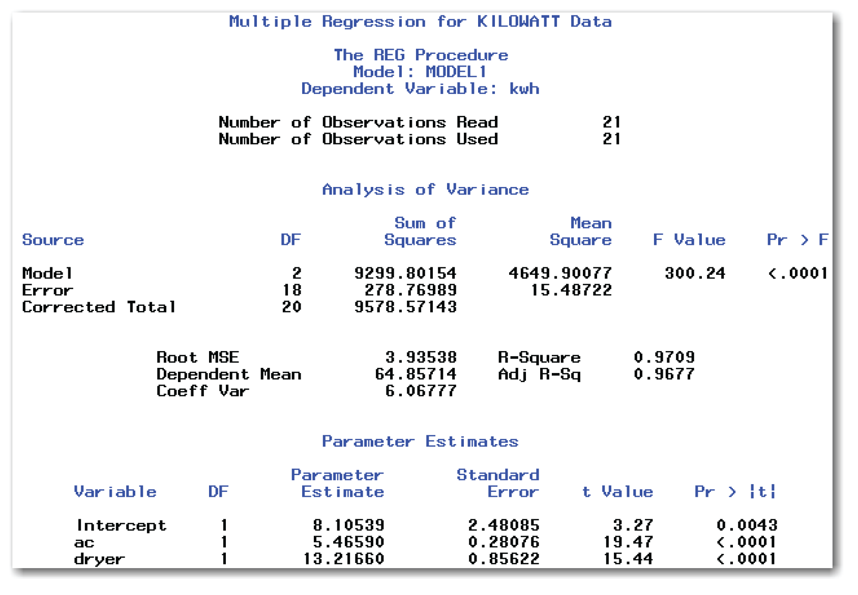
Figure 10.24 shows the same output tables as PROC REG shows for fitting a straight line or a curve. The next section explains how to interpret these results.

Understanding Results for Multiple Regression

Finding the Regression Equation

From the Parameter Estimates table in Figure 10.24, here is the fitted regression equation:

kwh = 8.11 + 5.47*ac + 13.22*dryer

The equation rounds the SAS parameter estimates to two decimal places. Interpret the coefficients as follows:

• The intercept is 8.11. It estimates the number of kilowatt-hours that were consumed on days when neither the air conditioner nor the dryer was used.
• The second term in the equation, 5.47*ac, indicates that the air conditioner uses 5.47 kwh an hour.
• The third term in the equation, 13.22*dryer, indicates that each dryer load uses 13.22 kwh.

You can specify values for ac and dryer, and then use the regression equation to predict the kwh that are consumed. PROC REG can create these predictions. See “Printing Predicted Values and Limits” later in this section.

Testing for Significance of Parameters

From the Parameter Estimates table in Figure 10.24, you conclude that all three coefficients are significantly different from 0. All three p-values are less than 0.05. The values for ac and dryer are both <.0001. These values provide overwhelming evidence of the significant effect of these variables on the kilowatt-hours that are consumed. The p-value for the intercept is 0.0043. This value provides evidence that a significant (nonzero) number of kilowatt-hours are consumed even when neither the air conditioner nor the dryer is used.

A significant regressor in multiple regression indicates that the variation explained by the regressor is significantly larger than the random variation in the data. For the kilowatt data, the electricity used by the ac and dryer is significantly larger than the random variation. Suppose the homeowner measured the number of times a small appliance, such as a coffee maker, was used. The amount of electricity the coffee maker uses is so small that it would probably not be detected. If you added coffeemaker to the model, you would probably find a large p-value, indicating that the coffee maker is not a significant source of variation.

Checking the Fit of the Model

In Figure 10.24, the Fit Statistics table shows an R-Square value of about 0.97, indicating that the fitted curve explains about 97% of the variation in the data. This is an excellent fit. Compare this fit with the R-Square value of 0.59 in Figure 10.12, which is for the model that contained only ac. Adding dryer to the model significantly improved the fit.

The Analysis of Variance table leads you to conclude that the fitted model with ac and dryer as regressors explains a significant amount of the variation in kwh. The p-value for the F test is <.0001. Statisticians typically examine the overall test of the fitted model before reviewing the details of parameter estimates.

Printing Predicted Values and Limits

Just as when you fit a straight line or a curve, you can print confidence limits for the mean, and confidence limits on an individual predicted value for multiple regression. Figure 10.25 shows the results from using the P, CLI, and CLM options in the MODEL statement.

Figure 10.25 for multiple regression shows the same SAS tables as Figure 10.19 for fitting a curve and Figure 10.13 for fitting a straight line.

Summarizing Multiple Regression

Multiple regression involves two or more independent variables. The same assumptions for fitting a straight line or a curve apply. In addition, the same analysis steps for fitting a straight line or a curve apply. Use PROC REG just as you use it for fitting a straight line or a curve, and interpret the results in the same way. You can print predicted values, confidence limits on the mean, and prediction limits.

After you fit the multiple regression, the next step is to perform diagnostics to check the fit of your model. Chapter 11 discusses a set of basic tools for regression diagnostics. The usual process of fitting a model is an iterative one. First, you fit a model, and then you look at the fit, revise the fit based on what you have learned from the diagnostic tools, look at the revised fit, and so on.

Summary

Key Ideas

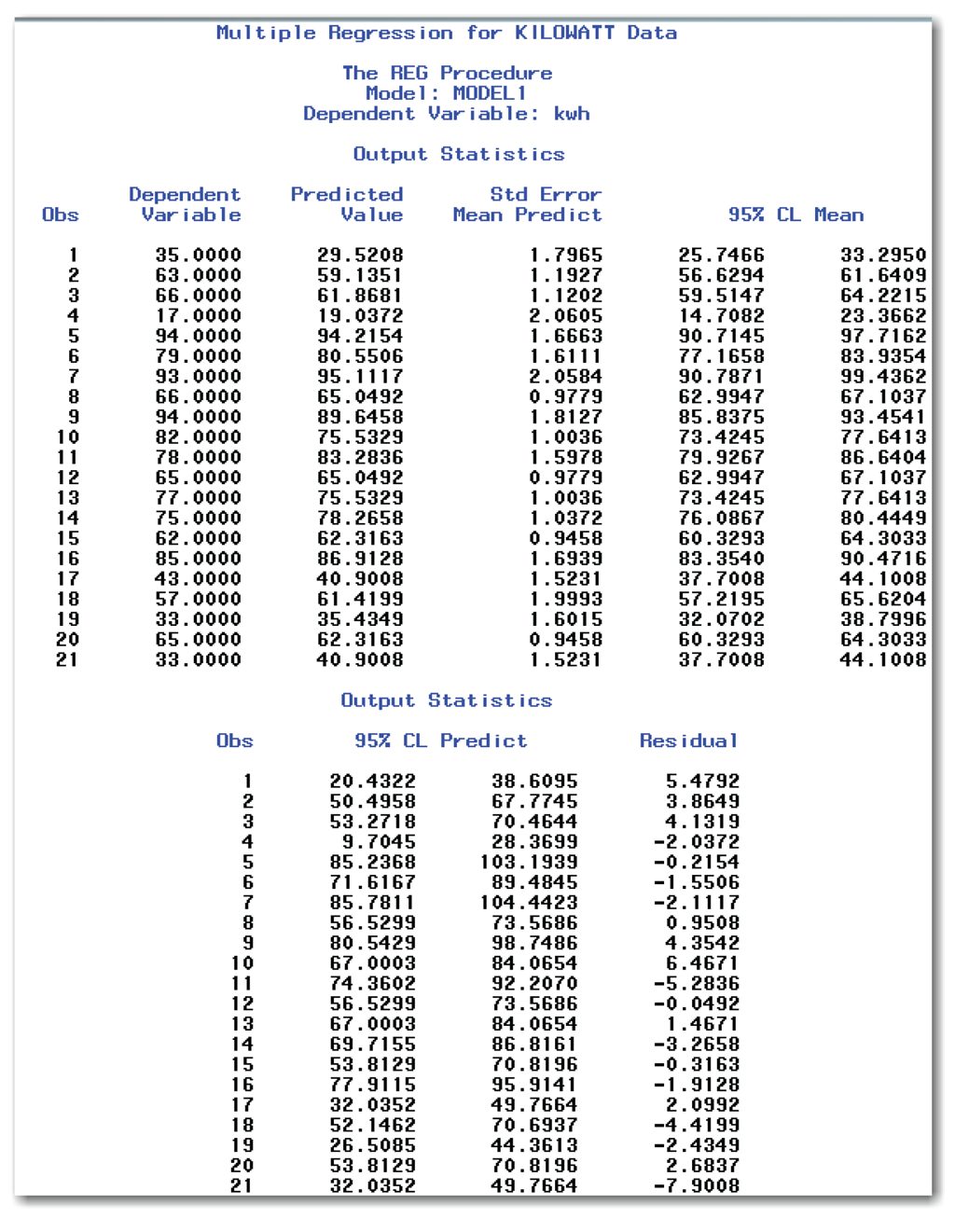
• Scatter plots show the relationship between two variables. A scatter plot matrix shows multiple relationships between pairs of variables.
• The Pearson correlation coefficient, r, measures the strength of the relationship between two variables. However, it does not describe the form of the relationship, and it does not show that one of the variables causes the other.
• PROC CORR creates scatter plots, a scatter plot matrix, summary statistics, correlation coefficients, and tests for the coefficients.
• Regression analysis describes relationships between variables. The simplest model fits a straight line that shows the relationship between one dependent variable (y) and one independent variable (x). Fitting a curve shows the relationship between one y variable, an x variable, and the square of x. Multiple regression shows the relationship between one y variable and two or more x variables.
• Least squares regression provides the best-fitting models. Here, the term “best-fitting” means that the fitted model minimizes the sum of squared differences between all of the data points and the fitted line, fitted curve, or multidimensional plane.
• Once regression analysis has been performed, use the fitted equation to predict future values at a given value of the independent variable.
• Prediction limits or confidence limits for individual values put bounds around a future value.
• Confidence limits for the mean put bounds around the mean value of the dependent variable at a given value of the independent variable.
• Plots of the actual data points, the regression equation itself, and prediction or confidence limits help you see how the regression equation fits the data.
• Regression analysis and regression diagnostics are intertwined. First, fit a model. Next, perform diagnostics to assess how well the model fits. Repeat this process until you find a suitable model. (Chapter 11 discusses performing diagnostics.)
• SAS provides many procedures that perform regression analysis. PROC REG is the simplest way to perform linear regression for lines, curves, and multiple regression. The procedure performs a test for the overall significance of the model, provides parameter estimates and significance tests for the estimates, and provides the R-Square statistic. Using options with PROC REG, you can print predicted values, prediction limits, and confidence limits for the mean. You can also produce plots that show the fitted line or curve.

Syntax

To summarize data with scatter plots and statistics

ODS GRAPHICS ON;

PROC CORR DATA=data-set-name options;

VAR variables;

ODS GRAPHICS OFF;

data-set-name

is the name of a SAS data set.

variables

are the variables you want to summarize. If you omit the variables from the VAR statement, then the procedure uses all numeric variables.

The PROC CORR statement options can be:

PLOTS=SCATTER(scatter-options)

creates a simple scatter plot for the variables.

SAS uses the first variable in the VAR statement for the x-axis, and the second variable for the y-axis. If you use more than two variables, then SAS creates a scatter plot for each pair of variables. The scatter-options can be one or more of the following:

NOINSET

suppresses an automatic summary that shows the number of observations and the correlation coefficient

ELLIPSE=NONE

suppresses the automatic prediction ellipse

If you use scatter-options, then the parentheses are required.

And, the PROC CORR statement options can be:

PLOTS=MATRIX(matrix-options)

creates a scatter plot matrix for the variables.

The matrix-options can be one or more of the following:

HISTOGRAM

adds a histogram for each variable along the diagonal of the matrix. This option is available starting with SAS 9.2.

NVAR=ALL

includes all variables in the scatter plot matrix. SAS automatically uses NVAR=5, so if your data has fewer than 5 variables, you can omit this option.

If you use matrix-options, then the parentheses are required.

You can use both PLOTS=SCATTER and PLOTS=MATRIX in the same PROC CORR statement.

To create correlation coefficients and tests

PROC CORR DATA=data-set-name options;

VAR variables;

The PROC CORR statement options can be as defined earlier and can also be:

NOMISS

excludes observations with missing values.

If you omit the variables from the VAR statement, then the procedure uses all numeric variables. Specify at least two variables for the output to be meaningful because the correlation of a variable with itself is always +1.

Other items in italic were defined earlier.

To perform regression to fit a line

PROC REG includes many other features and options that are not discussed in this chapter.

ODS GRAPHICS ON;

PROC REG DATA=data-set-name ALPHA=level plot-options;

ID variable;

MODEL y-variable=x-variable / P CLI CLM;

PRINT P CLI CLM;

PLOT y-variable*x-variable / options;

ODS GRAPHICS OFF;

data-set-name

is the name of a SAS data set.

variable

in the ID statement identifies observations.

y-variable

is the dependent variable.

x-variable

is the independent variable.

The PROC REG and MODEL statements are required. All other statements are optional.

PROC REG is an interactive procedure. The PROC REG, MODEL, and ID statements must be before the first RUN statement. The other statements can be before or after the first RUN statement. Use a QUIT statement to end the procedure when you are using PROC REG interactively.

In the PROC REG statement:

ALPHA=level

controls the confidence level for the limits. The value of level must be between 0 and 1. A level of 0.05 gives the automatic 95% limits.

The plot-options in the PROC REG statement require ODS graphics, and the plot-options discussed in this chapter require SAS 9.2 or later. The plot-options appropriate for a straight line are:

PLOTS(ONLY)=FIT(fit-options STATS=NONE)

ONLY

limits the plots to plots specified after the equal sign. PROC REG automatically produces several plots. Chapter 11 discusses the other plots, which are useful for regression diagnostics. When ONLY is used, the parentheses are required.

FIT

requests a plot with the data, fitted line, prediction limits, and confidence limits for the mean.

STATS=NONE

suppresses a table of statistics that automatically appears on the right side of the plot. When STATS=NONE is used, the parentheses are required.

The fit-options require parentheses. fit-options can be one of the following:

NOCLI

suppresses prediction limits.

NOCLM

suppresses confidence limits for the mean.

NOLIMITS

suppresses both prediction limits and confidence limits for the mean.

You can use the P, CLI, or CLM options in the MODEL or PRINT statement. You do not need to use the options in both statements. If you know in advance that you want the predicted values and limits, then use the options in the MODEL statement. If you want to check the fit of the line first, then use PROC REG interactively, and use the options in the PRINT statement.

P

requests predicted values. If you use the CLM or CLI option, then using P is not necessary.

CLI

requests prediction limits, which are confidence limits for an individual value.

CLM

requests confidence limits for the mean.

The PLOT statement can create a simple scatter plot, add the fitted line, and add limits, depending on the values of y-variable. (SAS documentation refers to graphics created with the PLOT statement as “traditional graphics.”) All plots should use the same x-variable. When you specify more than one y-variable, enclose the list of values for y-variable in parentheses. The y-variable can be the y-variable in the MODEL statement, or it can be one or more of the following statistical keywords:

P.

predicted value

LCL.

lower prediction limit

LCLM.

lower confidence limit for the mean

UCL.

upper prediction limit

UCLM.

upper confidence limit for the mean

The period after the statistical keyword is required.

The options in the PLOT statement can be:

NOSTAT

suppresses several automatic statistics that appear to the right of the graph.

CLINE=color

specifies the color of the regression line.

PRED

requests prediction limits.

CONF

requests confidence limits for the mean.

OVERLAY

overlays all y-variable requests onto a single plot.

To control the appearance of the plot, use SYMBOL statements:

SYMBOLn COLOR=color LINE=number;

n

has values from 1 to 6 for the straight-line regression plot. For the example code in this book, SYMBOL1 controls the color of the data points. SYMBOL2 controls the color and appearance of the fitted line. SYMBOL3 and SYMBOL4 control the color and appearance of the confidence limits for the mean. SYMBOL5 and SYMBOL6 control the color and appearance of the prediction limits.

COLOR=color

controls the color. This option in the SYMBOL statement overrides the CLINE= option.

LINE=number

controls the appearance of the line. For better graphs, use the same value for number for the upper and lower limits. SAS provides more than 45 line types.

To perform regression to fit a quadratic curve

Before fitting a curve, use a program statement in the DATA step to create the quadratic term in the regression equation:

quadratic-variable=independent-variable*independent-variable;

To fit a quadratic curve, and then print the predicted values and limits:

ODS GRAPHICS ON;

PROC REG DATA=data-set-name ALPHA=level plot-options;

ID variable;

MODEL y-variable=x-variable quadratic-variable / P CLI CLM;

PRINT P CLI CLM;

PLOT (y-variables)*x-variable / options;

ODS GRAPHICS OFF;

Items in italic were defined earlier. In the MODEL statement, the quadratic-variable is the new variable for the quadratic term. P, CLI, and CLM can be used in either the MODEL or PRINT statement.

The plot-options in the PROC REG statement require ODS graphics, and the plot-options discussed in this chapter require SAS 9.2 or later. The plot-options appropriate for a quadratic curve are:

PLOTS(ONLY)=PREDICTIONS(X=x-variable fit-options UNPACK)

ONLY

limits the plots to plots specified after the equal sign. PROC REG automatically produces several plots. Chapter 11 discusses the other plots, which are useful for regression diagnostics. When ONLY is used, the parentheses are required.

PREDICTIONS

requests a plot with the data, predicted curve, prediction limits, and confidence limits for the mean.The PREDICTIONS option is appropriate only for models that have terms for a single variable. The models can be a curve, cubic model, and so on. Models cannot have more than one x-variable.

X=x-variable

identifies the x-variable in the model.

UNPACK

separates the two plots that PROC REG automatically produces. Chapter 11 discusses the second plot, which is useful for regression diagnostics.

The fit-options require parentheses and are the same fit-options described for fitting a straight line.

The PLOT statement can create a simple scatter plot, add the fitted curve, and add limits, depending on the values of y-variables. (SAS documentation refers to graphics created with the PLOT statement as “traditional graphics.”) All plots should use the same x-variable. When you specify more than one y-variable, enclose the list of values for the y-variables in parentheses. The y-variables can be the y-variable in the MODEL statement, or it can be one or more of the following statistical keywords:

P.

predicted value

LCL.

lower prediction limit

LCLM.

lower confidence limit for the mean

UCL.

upper prediction limit

UCLM.

upper confidence limit for the mean

The period after the statistical keyword is required.

The options in the PLOT statement can be:

OVERLAY

places all plot requests on a single plot.

NOSTAT

suppresses several automatic statistics that appear to the right of the plot.

To control the appearance of the plot, use SYMBOL statements:

SYMBOLn VALUE=symbol COLOR=color LINE=number:

n

has values from 1 to 6. SYMBOL1 controls the appearance of the first y-variable in the PLOT statement. SYMBOL2 controls the appearance of the second y-variable, and so on.

VALUE=symbol

identifies the symbol used for the plotted point. SAS includes many automatic values, such as PLUS and DOT. You can also enter any single text character enclosed in double quotation marks.

COLOR= and LINE= are defined for fitting a line.

To perform multiple regression

To perform multiple regression, and then print the predicted values and limits:

PROC REG DATA=data-set-name ALPHA=level options;

ID variable;

MODEL y-variable=x-variable1 x-variable2 / P CLI CLM;

PRINT P CLI CLM;

Items in italic were defined earlier in the chapter. In the MODEL statement, x-variable1 is the first x-variable, x-variable2 is the second x-variable, and so on. P, CLI, and CLM can be used in either the MODEL or PRINT statement. With the exception of creating a simple scatter plot, ODS graphics and the PLOT statement are not appropriate for multiple regression.

As described in Chapter 4, you can use the ODS statement to control the output table that is printed. The table below identifies the ODS names of the PROC REG output tables and plots that are discussed in this chapter.

Example

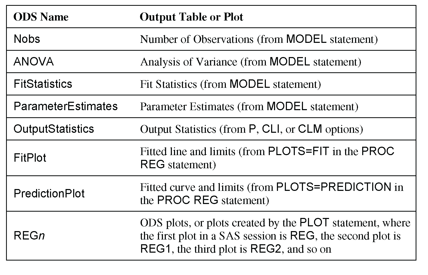
The program below produces the output shown in this chapter:

options ps=60 ls=80 nonumber nodate;

data kilowatt;

input kwh ac dryer @@;

datalines;

35 1.5 1 63 4.5 2 66 5.0 2 17 2.0 0 94 8.5 3 79 6.0 3

93 13.5 1 66 8.0 1 94 12.5 1 82 7.5 2 78 6.5 3 65 8.0 1

77 7.5 2 75 8.0 2 62 7.5 1 85 12.0 1 43 6.0 0 57 2.5 3

33 5.0 0 65 7.5 1 33 6.0 0

;

run;

ods select ScatterPlot;

ods graphics on;

proc corr data=kilowatt plots=scatter(noinset ellipse=none);

var ac kwh;

run;

ods graphics off;

ods graphics on;

ods select MatrixPlot;

proc corr data=kilowatt plots=matrix(histogram nvar=all);

var ac dryer kwh;

run;

ods graphics off;

ods select SimpleStats;

proc corr data=kilowatt;

var ac dryer kwh;

title 'Summary Statistics for KILOWATT Data Set';

run;

proc corr data=kilowatt;

var ac dryer kwh;

title 'Correlations for KILOWATT Data Set';

run;

data kilowatt2;

input kwh ac dryer @@;

datalines;

35 1.5 . 63 4.5 2 66 5.0 2 17 2.0 0 94 8.5 3 79 6.0 3

93 13.5 1 66 8.0 1 94 12.5 1 82 7.5 2 78 6.5 3 65 8.0 1

77 7.5 2 75 8.0 2 62 7.5 1 85 12.0 1 43 6.0 0 57 2.5 3

33 5.0 0 65 7.5 1 33 6.0 0

;

run;

proc corr data=kilowatt2;

var ac dryer kwh;

title 'Automatic Behavior with Missing Values for KILOWATT2';

run;

proc corr data=kilowatt2 nomiss;

var ac dryer kwh;

title 'NOMISS Option for KILOWATT2';

run;

proc reg data=kilowatt;

id ac;

model kwh=ac;

plot kwh*ac / nostat cline=red;

title 'Straight-line Regression for KILOWATT Data';

run;

print p clm cli;

run;

quit;

ods graphics on;

proc reg data=kilowatt plots(only)=fit(stats=none);

model kwh=ac / p clm cli;

title 'Straight-line Regression for KILOWATT Data';

run;

quit;

ods graphics off;

proc reg data=kilowatt;

model kwh=ac;

title 'Straight-line Regression for KILOWATT Data';

run;

symbol1 color=blue;

symbol2 color=red line=1;

symbol3 color=green line=2;

symbol4 color=green line=2;

symbol5 color=purple line=3;

symbol6 color=purple line=3;

plot kwh*ac / pred conf nostat;

run;

quit;

data engine;

input speed power @@;

speedsq=speed*speed;

datalines;

22.0 64.03 20.0 62.47 18.0 54.94 16.0 48.84 14.0 43.73

12.0 37.48 15.0 46.85 17.0 51.17 19.0 58.00 21.0 63.21

22.0 64.03 20.0 59.63 18.0 52.90 16.0 48.84 14.0 42.74

12.0 36.63 10.5 32.05 13.0 39.68 15.0 45.79 17.0 51.17

19.0 56.65 21.0 62.61 23.0 65.31 24.0 63.89

;

run;

ods graphics on;

ods select ScatterPlot;

proc corr data=engine plots=scatter(noinset ellipse=none);

var speed power;

title 'Scatterplot for ENGINE Data';

run;

ods graphics off;

proc reg data=engine;

id speed;

model power=speed speedsq / p cli clm;

title 'Fitting a Curve to the ENGINE Data';

run;

quit;

ods select OutputStatistics;

proc reg data=engine alpha=0.10;

model power=speed speedsq / p cli clm;

title '90% Limits for ENGINE Data';

run;

quit;

title;

ods graphics on;

ods select PredictionPlot;

proc reg data=engine alpha=0.10 plots(only)=predictions(x=speed unpack);

model power=speed speedsq ;

run;

quit;

ods graphics off;

proc reg data=engine alpha=0.10;

model power=speed speedsq ;

symbol1 value=plus color=blue;

symbol2 value=dot color=red;

symbol3 value="I" color=purple;

symbol4 value="M" color=green;

symbol5 value="I" color=purple;

symbol6 value="M" color=green;

plot (power p. lcl. lclm. ucl. uclm.)*speed / overlay nostat;

run;

quit;

proc reg data=kilowatt;

model kwh=ac dryer / p clm cli;

title 'Multiple Regression for KILOWATT Data';

run;

quit;

Special Topic: Line Printer Plots

Chapters 10 and 11 assume that you have the ability to create high-resolution graphics. These two chapters focus on graphs that you can create using either ODS graphics or high-resolution graphics. Each chapter includes a Special Topic section that discusses how to create line printer plots as an alternative. In some cases, you might not be able to create all of the plots in the chapter. Also, in some cases, SAS provides other procedures and other options. If you want line printer graphics, and the plots in this book do not meet your needs, then see the SAS documentation because graphic features that meet your needs might be available.

This section shows how to use PROC REG to create a line printer scatter plot of the data, a line printer scatter plot of the data and predicted values, and a line printer scatter plot that shows the data, predicted values, and limits.

To create a simple line printer scatter plot of the data with PROC REG:

options formchar="|----|+|---+=|-/<>*";

proc reg data=kilowatt lineprinter;

model kwh=ac;

plot kwh*ac="+";

title 'Straight-line Regression for KILOWATT Data';

run;

quit;

The OPTIONS statement includes the FORMCHAR= option, which specifies characters that are used for various aspects of the plot. SAS documentation recommends this specific value of the FORMCHAR= option to ensure consistent output on different computers.

The LINEPRINTER option specifies line printer plots. The PLOT statement specifies a simple scatter plot, and specifies that the data values appear as plus signs. You can specify any single character. Enclose the character in double quotation marks.

Figure ST10.1 shows the results.

To create a line printer scatter plot of the data and predicted values with PROC REG:

options formchar="|----|+|---+=|-/<>*";

proc reg data=kilowatt lineprinter;

model kwh=ac;

plot kwh*ac="+" p.*ac="p" / overlay;

title 'Straight-line Regression for KILOWATT Data';

run;

quit;

The PLOT statement includes two scatter plot requests. The OVERLAY option requests that the two scatter plots be placed on a single plot. P. specifies predicted values in the plot. For line printer plots, specify a symbol for each y*x request. Symbols will be helpful for understanding the plot. If symbols are omitted, then the plot shows the number of points at a given location as 1, 2, 3, and so on. The results can be confusing or difficult to interpret, especially for models where the predicted line or limits overlay the data values.

Figure ST10.2 shows the results.

Figure ST10.2 shows two question marks. PROC REG uses a question mark on a line printer plot when more than one value should be plotted. For this plot, the question marks indicate two places where the data value and the predicted value overlap and cannot be distinctly plotted.

To create a line printer scatter plot of the data, predicted values, and limits with PROC REG:

options formchar="|----|+|---+=|-/<>*";

proc reg data=kilowatt lineprinter;

model kwh=ac;

plot kwh*ac="+" p.*ac="p" lcl.*ac="I" lclm.*ac="M"

ucl.*ac="I" uclm.*ac="M" / overlay ;

title 'Straight-line Regression for KILOWATT Data';

run;

quit;

The PLOT statement includes several scatter plot requests. The OVERLAY option requests that all scatter plots be placed on a single plot. All of the output statistics in the plot requests end with a period. The plot requests use the letter “M” to represent the confidence limits for the mean, and “I” to represent the prediction limits.

Figure ST10.3 shows the results. Figure ST10.3 shows several question marks that indicate places where more than one point from the multiple plot requests overlap.

The general form of the statements to create line printer scatter plots in PROC REG is shown below:

OPTIONS FORMCHAR="|----|+|---+=|-/<>*";

PROC REG DATA=data-set-name LINEPRINTER options;

MODEL statement;

PLOT y*x="symbol" y*x="symbol" ... / OVERLAY;

Provide as many y*x plot requests as you want. The FORMCHAR= value ensures consistent output on different computers. OVERLAY requests that all of the y*x plot requests be placed on a single plot.

ENDNOTES