Chapter 9 Comparing More Than Two Groups
Suppose you are a greenhouse manager and you want to compare the effects of six different fertilizers on the growth of geraniums. You have 30 plants, and you randomly assigned five plants to each of the six fertilizer groups. You carefully controlled other factors: you used the same type of soil for all 30 plants, you made sure that they all received the same number of hours of light each day, and you applied the fertilizers on the same day and in the same amounts to all 30 plants. At the end of this designed experiment, you measured the height of each plant. Now, you want to compare the six fertilizer groups in terms of plant height. This chapter discusses the analysis of this type of situation. This chapter discusses the following topics:
- summarizing data from more than two groups
- building a statistical test of hypothesis to compare data in several groups
- performing a one-way analysis of variance
- performing a Kruskal-Wallis test
- exploring group differences with multiple comparison procedures
The methods that are discussed are appropriate when each group consists of measurements of different items. The methods are not appropriate when “groups” consist of measurements of the same item at different times (for example, if you measured the same 15 plants at two, four, and six weeks after applying fertilizer). (This is a repeated measures design. See Appendix 1, “Further Reading,” for information.)
This chapter discusses analysis methods for an ordinal or continuous variable as the measurement variable. The variable that classifies the data into groups should be nominal and can be either character or numeric.
Summarizing Data from Multiple Groups
Creating Comparative Histograms for Multiple Groups
Creating Side-by-Side Box Plots for Multiple Groups
Building Hypothesis Tests to Compare More Than Two Groups
Using Parametric and Nonparametric Tests
Performing the Analysis of Variance
Analysis of Variance with Unequal Variances
Performing a Kruskal-Wallis Test
Understanding Multiple Comparison Procedures
Performing Pairwise Comparisons with Multiple t-Tests
Performing the Tukey-Kramer Test
Using Dunnett’s Test When Appropriate
Summarizing Multiple Comparison Procedures
Summarizing Data from Multiple Groups
This section explains how to summarize data from multiple groups. These methods do not replace formal statistical tests, but they do provide a better understanding of the data and can help you understand the results from formal statistical tests.
Before you can summarize data, you need data to be in a SAS data set. Then, you check the data set for errors. For a small data set, you can print the data and compare the printout with the data that you collected. For a larger data set, you can use the methods discussed in Chapter 4. You can use the same SAS procedures to check for errors and to summarize the data.
Suppose you have data from an investigation of teachers’ salaries for different subject areas. You want to know whether the teachers’ salaries are significantly different for different subject areas. Table 9.1 shows the data.[1]
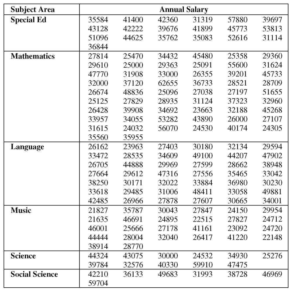
This data is available in the salary data set in the sample data for the book. The statements in the “Example” section at the end of the chapter create a SAS data set for the teacher salary data in Table 9.1.
To summarize the data in SAS, you can use the same methods that you use for two independent groups.
- PROC MEANS with a CLASS statement for a concise summary.
- PROC UNIVARIATE with a CLASS statement for a detailed summary.This summary contains output tables for each value of the class-variable. You can use the PLOT option to create line printer plots for each value of the class-variable.
- PROC UNIVARIATE with a CLASS statement and HISTOGRAM statement for comparative histograms.
- PROC CHART for side-by-side bar charts. These bar charts are a low-resolution alternative to comparative histograms.
- PROC BOXPLOT for side-by-side box plots.
Following the same approach as you do for two groups, use PROC MEANS. The SAS statements below produce a concise summary of the data:
proc means data=salary;
class subjarea;
var annsal;
title 'Brief Summary of Teacher Salaries';
run;
Figure 9.1 shows the results.

Figure 9.1 shows descriptive statistics for each group. Social Science teachers have the highest average annual salary, and Music teachers have the lowest average annual salary. The sizes of the groups vary widely, from only seven Social Science teachers to 56 Mathematics teachers.
Looking at the averages and standard deviations, you might think that there are salary differences for the different subject areas. To find out whether these differences are greater than what could have happened by chance requires a statistical test.
Creating Comparative Histograms for Multiple Groups
Chapter 8 discussed comparative histograms for two independent groups. You can use the same approach for multiple groups. PROC UNIVARIATE automatically creates two rows of histograms on a single page. This is ideal for two independent groups, but PROC UNIVARIATE prints on multiple pages when there are more than two groups. For multiple groups, you can use the NROWS= option to display all of the groups on a single page. For the teacher salary data, type the following:
proc univariate data=salary noprint;
class subjarea;
var annsal;
histogram annsal / nrows=6;
title 'Comparative Histograms by Subject Area';
run;
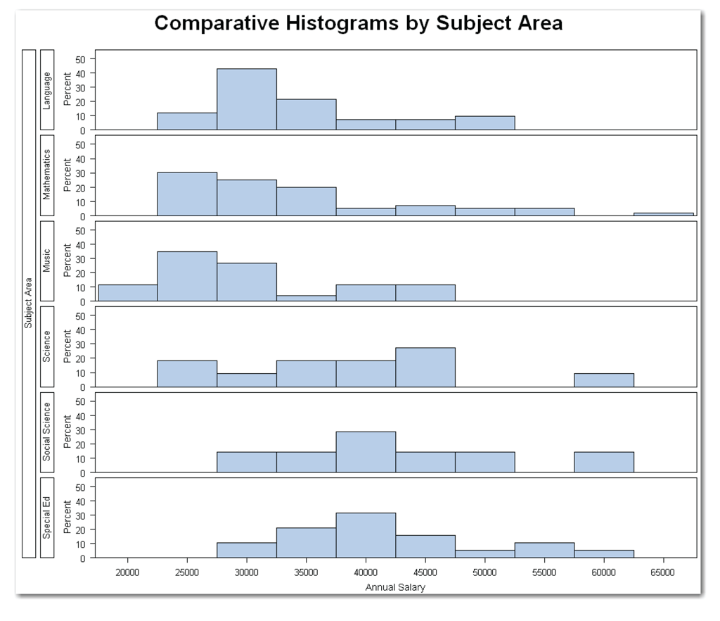
The statements use the NOPRINT option to suppress the display of the usual output tables. The NROWS=6 option specifies six rows of histograms, one row for each of the six subject areas. Figure 9.2 shows the results.
The histograms show the different distributions of salaries for the subject areas. Although there might be salary differences in the subject areas, you don’t know whether these differences are greater than what could have happened by chance.
The histograms also highlight potential outliers to investigate. For this data, the Mathematics group shows a bar separated from the other bars. If you investigate, you find that this is a valid data value for the teacher earning $62,655.
The general form of the statements to create comparative histograms for multiple groups using PROC UNIVARIATE is shown below:
PROC UNIVARIATE DATA=data-set-name NOPRINT;
CLASS class-variable;
VAR measurement-variables;
HISTOGRAM measurement-variables / NROWS=value;
data-set-name is the name of a SAS data set, class-variable is a variable that classifies the data into groups, and measurement-variables are the variables that you want to summarize.
To compare groups, the CLASS statement is required. The class-variable can be character or numeric and should be nominal. If you omit the measurement-variables from the VAR statement, then the procedure uses all numeric variables.
You can use the options described in Chapters 4 and 5 with PROC UNIVARIATE and a CLASS statement. You can omit the NOPRINT option and create the detailed summary and histograms at the same time.
The NROWS= option controls the number of histograms that appear on a single page. SAS automatically uses NROWS=2. For your data, choose a value equal to the number of groups.
If any option is used in the HISTOGRAM statement, then the slash is required.
Creating Side-by-Side Box Plots for Multiple Groups
Chapter 8 discussed side-by-side box plots for two independent groups. You can use the same approach for multiple groups. When group sizes vary widely, the BOXWIDTHSCALE=1 and BWSLEGEND options can be helpful. For the teacher salary data, type the following:
proc sort data=salary;
by subjarea;
run;
proc boxplot data=salary;
plot annsal*subjarea / boxwidthscale=1 bwslegend;
title 'Comparative Box Plots by Subject Area';
run;
PROC BOXPLOT expects the data to be sorted by the variable that classifies the data into groups. If your data is already sorted, you can omit the PROC SORT step.
The BOXWIDTHSCALE=1 option scales the width of the boxes based on the size of each group. The BWSLEGEND option adds a legend to the bottom of the comparative box plot. The legend explains the varying box widths. Figure 9.3 shows the results.

The box plots help you visualize the differences between the averages for the six subject areas. Looking at the median (the center line of the box), you can observe differences in the subject areas. But, you don’t know whether these differences are greater than what could have happened by chance. To find out requires a statistical test.
Using BOXWIDTHSCALE=1 scales the widths of the boxes based on the sample size for each group. You can see the small sizes for the Science, Social Science, and Special Ed subject areas.
Looking at the box plots highlights the wide range of points for several subject areas. When checking the data for errors, you investigate the extreme values (using PROC UNIVARIATE) and compare them with the original data. You find that all of the data values are valid.
The general form of the statements to create side-by-side box plots for multiple groups using PROC BOXPLOT is shown below:
PROC BOXPLOT DATA=data-set-name;
PLOT measurement-variable*class-variable
/ BOXWIDTHSCALE=1 BWSLEGEND;
Items in italic were defined earlier in the chapter. Depending on your data, you might need to first sort by the class-variable before creating the plots. The asterisk in the PLOT statement is required.
The BOXWIDTHSCALE=1 option scales the width of the boxes based on the sample size of each group. The BWSLEGEND option adds a legend to the bottom of the comparative box plot. The legend explains the varying box widths. If either option is used, then the slash is required. You can use the options alone or together, as shown above.
Building Hypothesis Tests to Compare More Than Two Groups
So far, this chapter has discussed how to summarize differences between groups. When you start a study, you want to know how important the differences between groups are, and whether the differences are large enough to be statistically significant. In statistical terms, you want to perform a hypothesis test. This section discusses hypothesis testing when comparing multiple groups. (See Chapter 5 for the general idea of hypothesis testing.)
When comparing multiple groups, the null hypothesis is that the means for the groups are the same, and the alternative hypothesis is that the means are different. The salary data has six groups. In this case, the notation is the following:
Ho: μA = μB = μC = μD =μE = μF
Ha: at least two means are different
Ho indicates the null hypothesis, Ha indicates the alternative hypothesis, and μA, μB, μC, μD, μE, and μF are the population means for the six groups. The alternative hypothesis does not specify which means are different from one another. It specifies simply that there are some differences among the means. The preceding notation shows the hypotheses for comparing six groups. For more groups or fewer groups, add or delete the appropriate number of means in the notation.
In statistical tests that compare multiple groups, the hypotheses are tested by partitioning the total variation in the data into variation due to differences between groups, and variation due to error. The error variation does not refer to mistakes in the data. It refers to the natural variation within a group (and possibly to the variation due to other factors that were not considered). The error variation is sometimes called the within group variation. The error variation represents the natural variation that would be expected by chance. If the variation between groups is large relative to the error variation, the means are likely to be different.
Because the hypothesis test analyzes the variation in the data, it is called an analysis of variance and is abbreviated as ANOVA. The specific case of analyzing only the variation between groups and the variation due to error is called a one-way ANOVA. Figure 9.4 shows how the total variation is partitioned into variation between groups and variation due to error.

Another way to think about this idea is to use the following model:
variation in the measurement-variable=
(variation between levels of the class-variable)+
(variation within levels of the class-variable)
Abbreviated for the salary example, this model is the following:
annsal = subjarea + error
For a one-way ANOVA, the only term in the model is the term for the class-variable, which identifies the groups.
Using Parametric and Nonparametric Tests
In this book, the term “ANOVA” refers specifically to a parametric analysis of variance, which can be used if the assumptions seem reasonable. If the assumptions do not seem reasonable, use the nonparametric Kruskal-Wallis test, which has fewer assumptions. In general, if the assumptions for the parametric ANOVA seem reasonable, use the ANOVA. Although nonparametric tests like the Kruskal-Wallis test have fewer assumptions, these tests typically are less powerful in detecting differences between groups.
If all of the groups have the same sample size, the data is balanced. If the sample sizes are different, the data is unbalanced.
This distinction can be important for follow-up tests to an ANOVA, or for other types of experimental designs. However, for a one-way ANOVA or a Kruskal-Wallis test, you don’t need to worry about whether the data is balanced. SAS automatically handles balanced and unbalanced data correctly in these analyses.
In either an ANOVA or a Kruskal-Wallis test, there are two possible results: the p-value is less than the reference probability, or it is not. (See Chapter 5 for discussions on significance levels and on understanding practical significance and statistical significance.)
Groups Significantly Different
If the p-value is less than the reference probability, the result is statistically significant, and you reject the null hypothesis. You conclude that the means for the groups are significantly different. You don’t know which means are different from one another; you know simply that some differences exist in the means.
Your next step might be to use a multiple comparison procedure to further analyze the differences between groups. An alternative to using a multiple comparison procedure is performing comparisons that you planned before you collected data. If you have certain comparisons that you know you want to make, consult a statistician for help in designing your study.
Groups Not Significantly Different
If the p-value is greater than the reference probability, the result is not statistically significant, and you fail to reject the null hypothesis. You conclude that the means for the groups are not significantly different.
Do not “accept the null hypothesis” and conclude that the means for the groups are the same.
This distinction is very important. You do not have enough evidence to conclude that the means are the same. The results of the test indicate only that the means are not significantly different. You never have enough evidence to conclude that the population is exactly as described by the null hypothesis. In statistical hypothesis testing, do not accept the null hypothesis. Instead, either reject or fail to reject the null hypothesis.
A larger sample might have led you to conclude that the groups are different. Perhaps there are other factors that were not controlled, and these factors influenced the experiment enough to obscure the differences between the groups. For a more detailed discussion of hypothesis testing, see Chapter 5.
This section discusses the assumptions for a one-way ANOVA, how to test the assumptions, how to use SAS, and how to interpret the results. The steps for performing the analyses to compare multiple groups are the same as the steps for comparing two groups:
1. Create a SAS data set.
2. Check the data set for errors.
3. Choose the significance level for the test.
4. Check the assumptions for the test.
5. Perform the test.
6. Make conclusions from the test results.
Steps 1 and 2 have been done. For step 3, compare the groups at the 10% significance level. For significance, the p-value needs to be less than the reference probability value of 0.10.
The assumptions for an analysis of variance are the following:
- Observations are independent. The measurement of one observation cannot affect the measurement of another observation.
- Observations are a random sample from a population with a normal distribution. If there are differences between groups, there might be a different normal distribution for each group. (The assumption of normality requires that the measurement variable is continuous. If your measurement variable is ordinal, go to the section on the Kruskal-Wallis test later in this chapter.)
- Groups have equal variances.
The assumption of independent observations seems reasonable because the annual salary for one teacher is unrelated to and unaffected by the annual salary for another teacher.
The assumption of normality is difficult to verify. Testing this assumption requires performing a test of normality on each group. For the subject areas that have a larger number of observations, this test could be meaningful. But, for the subject areas that have only a few observations, you don’t have enough data to perform an adequate test. And, because you need to verify the assumption of normality in each group, this is difficult. For now, assume normality, and perform an analysis of variance.
In general, if you have additional information (such as other data) that indicates that the population is normally distributed, and if your data is a representative sample of the population, you can usually proceed based on the idea that the assumption of normality seems reasonable. In addition, the analysis of variance works well even for data from non-normal populations. However, if you are uncomfortable with proceeding, or if you do not have other data or additional information about the distribution of measurements, or if you have large groups that don’t seem to be samples from normally distributed populations, you can use the Kruskal-Wallis test.
The assumption of equal variances seems reasonable. Look at the similarity of the standard deviations in Figure 9.1, and the relatively similar heights of the box plots in Figure 9.3. The standard deviations vary, but it is difficult to determine whether the variability is because of true changes in the variances or because of sample sizes. Look at the differences in sample sizes for the different subject areas. There are 7 observations for Social Science, and 56 observations for Mathematics. The standard deviations for these subject areas are relatively similar. However, compare the standard deviations for Social Science and Special Ed. It’s more difficult to determine whether the difference in standard deviations (which is larger) is because of true changes in the variances or because of less precise estimates of variances as a result of smaller sample sizes. For now, assume equal variances, and perform an analysis of variance. See “Analysis of Variance with Unequal Variances” later in the chapter for an alternative approach.
Performing the Analysis of Variance
SAS includes many procedures that perform an analysis of variance in different situations. PROC ANOVA is the simplest of these procedures and assumes that the data is balanced. For balanced data, PROC ANOVA is more efficient (runs faster) than the other SAS procedures for analysis of variance.
For the special case of a one-way ANOVA, you can use PROC ANOVA for both balanced and unbalanced data. In general, however, you should use PROC GLM for unbalanced data.
To perform a one-way ANOVA for the salary data, type the following:
proc anova data=salary;
class subjarea;
model annsal=subjarea;
title 'ANOVA for Teacher Salaries';
run;
The CLASS statement identifies the variable that classifies the data into groups. The MODEL statement describes the relationship that you want to investigate. In this case, you want to find out how much of the variation in the salaries (annsal) is due to differences between the subject areas (subjarea). Figure 9.5 shows the results.
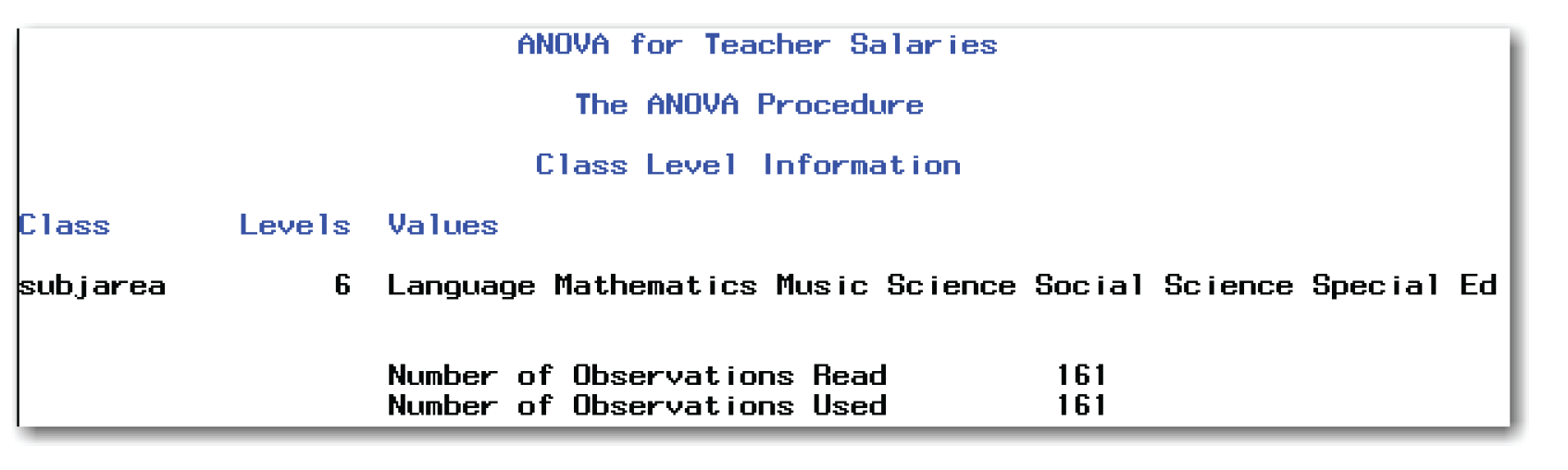
Figure 9.5 Analysis of Variance for Salary Data (continued)
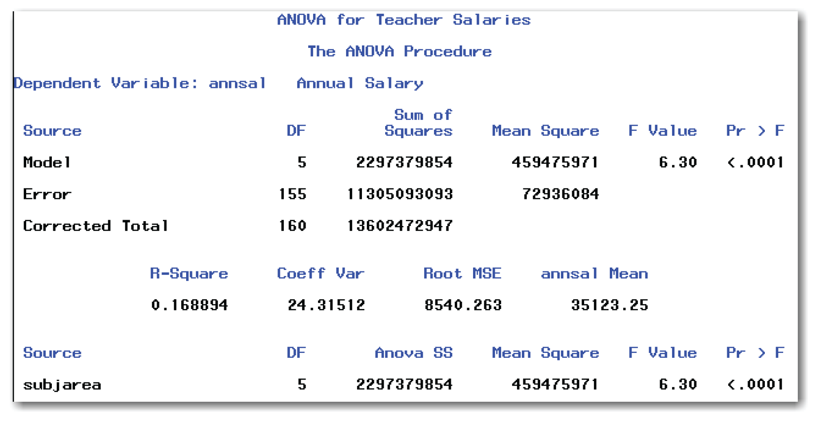
Figure 9.5 shows the details of the one-way ANOVA. First, answer the research question, “Are the mean salaries different for subject areas?”
Finding the p-value
To find the p-value in the salary data, look in Figure 9.5 at the line listed in the Source column labeled subjarea. Then look at the column labeled Pr > F. The number in this column is the p-value for comparing groups. Figure 9.5 shows a value of <.0001. Because 0.0001 is less than the reference probability of 0.10, you conclude that the mean salaries for subject areas are significantly different.
To find the p-value in your data, find the Source line labeled with the name of the variable in the CLASS statement. The p-value is listed in the Pr > F column. It gives you the results of the hypothesis test for comparing the means of multiple groups.
In general, to perform the test at the 5% significance level, you conclude that the means for the groups are significantly different if the p-value is less than 0.05. To perform the test at the 10% significance level, you conclude that the means for the groups are significantly different if the p-value is less than 0.10. Conclusions for tests at other significance levels are made in a similar manner.
Understanding the First Page of Output
The first page of output contains two tables. The Class Level table identifies the class-variable, number of levels for this variable, and values for this variable. The Number of Observations table identifies the number of observations read from the data set, and the number of observations that PROC ANOVA used in analysis. For data for a one-way ANOVA with no missing values, these two numbers will be the same.
Understanding the Second Page of Output
The first line of the second page of output identifies the measurement-variable with the label Dependent Variable. For the salary data, the variable is annsal. Because the variable has a label in the data set, PROC ANOVA also displays the label. For your particular data, the procedure will display the measurement-variable name and might display the label.
After this first heading, the second page of output contains three tables. The Overall ANOVA table shows the analysis with terms for Model and Error. The Fit Statistics table contains several statistics. The Model ANOVA table contains the one-way ANOVA and the p-value.
For a one-way ANOVA, the only term in the model is class-variable, which identifies the variable that classifies the data into groups. As a result, for a one-way ANOVA, the p-values in the Overall ANOVA table and in the Model ANOVA table are the same.
The list below describes items in the Overall ANOVA table:
Source
lists the sources of variation in the data. For a one-way ANOVA, this table summarizes all sources of variation. Because the model has only one source of variation (the groups), the values in the line for Model in this table match the corresponding values in the Model ANOVA table.
DF
is degrees of freedom. For a one-way ANOVA, the DF for Corrected Total is the number of observations minus 1 (160=161-1). The DF for Model is the number of groups minus 1. For the salary data, 5=6-1. For your data, the DF for Model will be one less than the number of groups. The DF for Error is the difference between these two values (155=160-5).
Sum of Squares
Measures the amount of variation that is attributed to a given source. In this table, the Sum of Squares measures the amount of variation for the entire model. Sum of Squares is often abbreviated as SS. For the one-way ANOVA, the Model SS and the subjarea SS are the same. This is not true for more complicated models.
The Sum of Squares for the Model and Error sum to be equal to the Corrected Total Sum of Squares.
Mean Square
is the Sum of Squares divided by DF. SAS uses Mean Square to construct the statistical test for the model.
F Value
is the value of the test statistic. The F Value is the Mean Square for Model divided by the Mean Square for Error.
Pr > F
gives the p-value for the test for the overall model. Because the model for an ANOVA contains only one term, this p-value is the same as the p-value to compare groups.
The list below describes items in the Fit Statistics table:
R-square
for a one-way analysis of variance, describes how much of the variation in the data is due to differences between groups. This number ranges from 0 to 1; the closer it is to 1, the more variation in the data is due to differences between groups.
Coeff Var
gives the coefficient of variation, which is calculated by multiplying the standard deviation by 100, and then dividing this value by the average.
Root MSE
gives an estimate of the standard deviation after accounting for differences between groups. This is the square root of the Mean Square for Error.
annsal Mean
gives the overall average for the measurement-variable. For your data, the value will list the name of your measurement-variable.
The list below describes items in the Model ANOVA table:
Source
lists the sources of variation in the data. For a one-way ANOVA, this table identifies the variable that classifies the data into groups (subjarea in this example). Because the model has only one source of variation (the groups), the values for subjarea in this table match the corresponding values in the Overall ANOVA table.
DF
is degrees of freedom for the variable that classifies the data into groups (subjarea in this example). The value should be the same as DF for Model because the model has only one source of variation (the groups).
Anova SS
in this table, the Anova SS measures the amount of variation that is attributed to the variable that classifies the data into groups (subjarea in this example).
Mean Square
is the Anova SS divided by DF. SAS uses Mean Square to construct the statistical test to compare groups.
F Value
is the value of the test statistic. This is the Mean Square for the variable that classifies the data into groups (subjarea in this example) divided by the Mean Square for Error. An analysis of variance involves partitioning the variation and testing to find out how much variation is because of differences between groups. Partitioning is done by the F test, which involves calculating an F-value from the mean squares.
Pr > F
gives the p-value for the test to compare groups. Compare this value with the reference probability value that you selected before you ran the test.
Analysis of Variance with Unequal Variances
Earlier, this chapter discussed the assumption of equal variances, and an ANOVA was performed after looking at standard deviations and box plots. Some statisticians perform an ANOVA without testing for equal variances. Unless the variances in the groups are very different, or unless there are many groups, an ANOVA detects appropriate differences when all of the groups are about the same size.
SAS provides tests for unequal variances, and provides an alternative to the usual ANOVA when the assumption of equal variances does not seem reasonable.
For the salary data, suppose you want to test for equal variances at the 10% significance level. This decision gives a reference probability of 0.10. To test the assumption of equal variances in SAS, type the following:
proc anova data=salary;
class subjarea;
model annsal=subjarea;
means subjarea / hovtest;
title 'Testing for Equal Variances';
run;
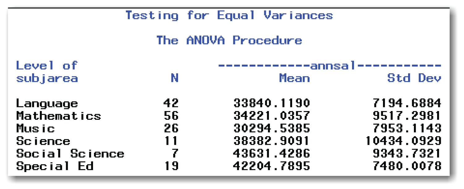
These statements produce the results shown in Figure 9.5. The MEANS statement is new and produces the results shown in Figures 9.6 and 9.7.
The HOVTEST option tests for homogeneity of variances, which is another way of saying equal variances. SAS automatically performs Levene’s test for equal variances. Levene’s test has a null hypothesis that the variances are equal, and an alternative hypothesis that they are not equal. This test is most widely used by statisticians and is considered to be the standard test. SAS provides options for other tests, which are discussed in the SAS documentation.
Figure 9.6 shows descriptive statistics for each of the groups.
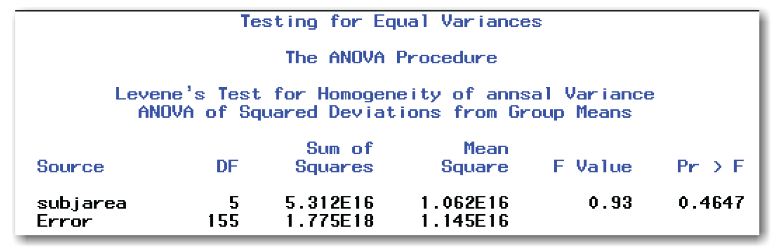
To find the p-value, find the line labeled subjarea and look at the column labeled Pr > F. The number in this column is the p-value for testing the assumption of equal variances. Because the p-value of 0.4647 is much greater than the significance level of 0.10, do not reject the null hypothesis of equal variances for the groups. In fact, there is almost a 47% chance that this result occurred by random chance. You conclude that there is not enough evidence that the variances in annual salaries for the six subject areas are significantly different. You proceed, based on the assumption that the variances for the groups are equal.
In general, compare the p-value to the reference probability. If the p-value is greater than the reference probability, proceed with the ANOVA based on the assumption that the variances for the groups are equal. If the p-value is less than the reference probability, use the Welch ANOVA (discussed in the next topic) to compare the means of the groups.
This table also contains other details for Levene’s test, including the degrees of freedom, sum of squares, mean square, and F-value. See the SAS documentation for more information about Levene’s test.
Welch’s ANOVA tests for differences in the means of the groups, while allowing for unequal variances across groups. To perform Welch’s ANOVA in SAS, type the following:
proc anova data=salary;
class subjarea;
model annsal=subjarea;
means subjarea / welch;
title 'Welch ANOVA for Salary Data';
run;
These statements produce the results shown in Figures 9.5 and 9.6. The WELCH option in the MEANS statement performs the Welch’s ANOVA and produces the output in Figure 9.8.

Find the column labeled Pr > F under the Welch’s ANOVA heading. The number in this column is the p-value for testing for differences in the means of the groups. For the salary data, this value is 0.0002. You conclude that the mean salaries are significantly different across subject areas. For the salary data, this is for example only. You already know that the assumption of equal variances seems reasonable and that you can apply the usual ANOVA test.
The F Value gives the value of the test statistic. DF gives the degrees of freedom for the Source. For the class-variable (subjarea in Figure 9.8), the degrees of freedom are calculated as the number of groups minus 1. The degrees of freedom for Error has a more complicated formula. See the SAS documentation for formulas.
If Welch’s ANOVA test is used, then multiple comparison procedures (discussed later in the chapter) are not appropriate.
The general form of the statements to perform a one-way ANOVA, test the assumption of equal variances, and perform Welch’s ANOVA using PROC ANOVA is shown below:
PROC ANOVA DATA=data-set-name;
CLASS class-variable;
MODEL measurement-variable=class-variable;
MEANS class-variable / HOVTEST WELCH;
Items in italic were defined earlier in the chapter.
The PROC ANOVA, CLASS, and MODEL statements are required.
The HOVTEST option performs a test for equal variances across the groups. The WELCH option performs the Welch ANOVA when there are unequal variances. If either option is used, then the slash is required. You can use the options alone or together, as shown above.
You can use the BY statement in PROC ANOVA to perform several one-way ANOVAs for levels of another variable. However, another statistical analysis might be more appropriate. Consult a statistical text or a statistician before you do this analysis.
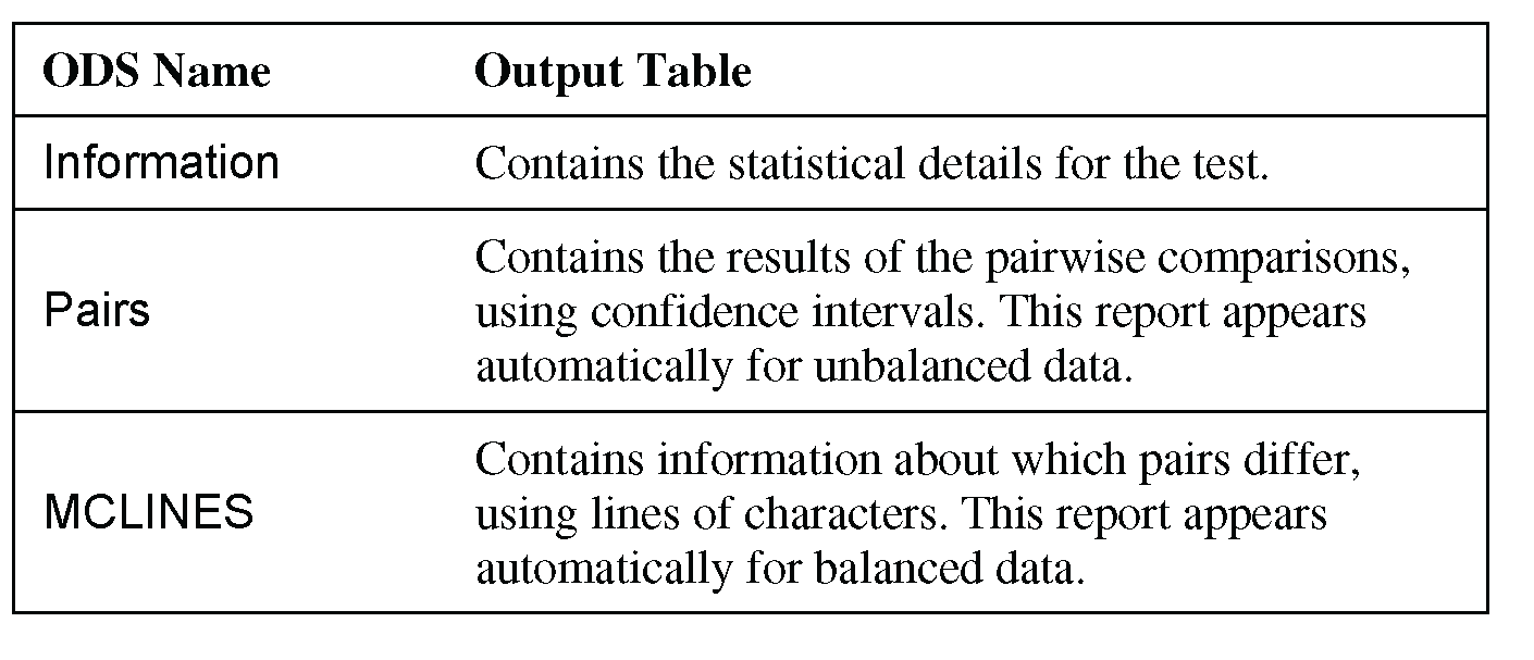
As discussed in Chapter 4, you can use the ODS statement to choose the output tables to display. Table 9.2 identifies the output tables for PROC ANOVA.

Performing a Kruskal-Wallis Test
The Kruskal-Wallis test is a nonparametric analogue to the one-way ANOVA. Use this test when the normality assumption does not seem reasonable for your data. If you do have normally distributed data, this test can be conservative and can fail to detect differences between groups. The steps of the analysis are the same as for an ANOVA.
In practice, the Kruskal-Wallis test is used for ordinal or continuous variables. The null hypothesis is that the populations for the groups are the same.
You have already performed the first three steps of the analysis. As for the ANOVA, use a 10% significance level to test for differences between groups.
To perform the fourth step for analysis, check the assumptions for the test.
The only assumption for this test is that the observations are independent.
For the salary data, this assumption seems reasonable because the salary for one teacher is independent of the salary for another teacher.
To perform a Kruskal-Wallis test with SAS, use PROC NPAR1WAY:
proc npar1way data=salary wilcoxon;
class subjarea;
var annsal;
title 'Nonparametric Tests for Teacher Salary Data';
run;
The CLASS statement identifies the variable that classifies the data into groups. The VAR statement identifies the variable that you want to analyze. Figure 9.9 shows the results.
Figure 9.9 shows two output tables. The first table contains Wilcoxon scores, and has the same information that Chapter 8 discussed for the Wilcoxon Rank Sum test. (In Chapter 8, see “Using PROC NPAR1WAY for the Wilcoxon Rank Sum Test” for details.) You can think of the Kruskal-Wallis test as an extension of the Wilcoxon Rank Sum test for more than two groups. The second table contains the results of the Kruskal-Wallis test.

First, answer the research question, “Are the mean salaries different for subject areas?”
Finding the p-value
Find the line labeled Pr > Chi-Square in Figure 9.9. The number in this line is the p-value for comparing groups. Figure 9.9 shows a value of <.0001. Because 0.0001 is less than the reference probability of 0.10, you can conclude that the mean salaries are significantly different across subject areas.
In general, to interpret results, look at the p-value in Pr > Chi-Square. If the p-value is less than the significance level, you conclude that the means for the groups are significantly different. If the p-value is greater, you conclude that the means for the groups are not significantly different. Do not conclude that the means for the groups are the same.
Understanding Other Items in the Tables
See “Using PROC NPAR1WAY for the Wilcoxon Rank Sum Test” in Chapter 8 for details on the items in the Wilcoxon Scores table.
The Kruskal-Wallis Test table displays the statistic for the test (Chi-Square) and the degrees of freedom for the test (DF). The degrees of freedom are calculated by subtracting 1 from the number of groups. For the salary data, this is 5=6–1.
The general form of the statements to perform tests to compare multiple groups using PROC NPAR1WAY is shown below:
PROC NPAR1WAY DATA=data-set-name WILCOXON;
CLASS class-variable;
VAR measurement-variables;
Items in italic were defined earlier in the chapter.
The CLASS statement is required.
While the VAR statement is not required, you should use it. If you omit the VAR statement, then PROC NPAR1WAY performs analyses for every numeric variable in the data set.
You can use the BY statement in PROC NPAR1WAY to perform several analyses for levels of another variable. However, another statistical analysis might be more appropriate. Consult a statistical text or a statistician before you do this analysis.
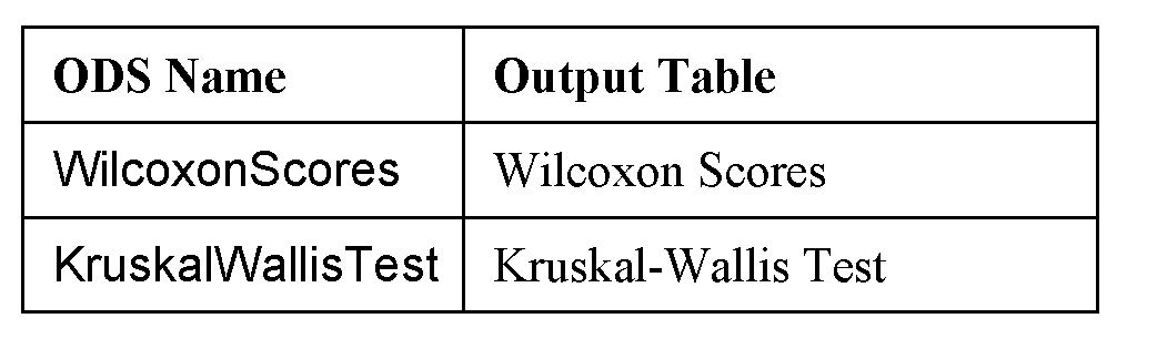
As discussed in Chapter 4, you can use the ODS statement to choose the output tables to display. Table 9.3 identifies the output tables for PROC NPAR1WAY and the Kruskal-Wallis test.
Understanding Multiple Comparison Procedures
When you conclude that the means are significantly different after performing an ANOVA, you still don’t know enough detail to take action. Which means differ from other means? At this point, you know only that some means differ from other means. Your next step is to use a multiple comparison procedure, or a test that makes two or more comparisons of the group means.
Many statisticians agree that multiple comparison procedures should be used only after a significant ANOVA test. Technically, this significant ANOVA test is called a “prior significant F test” because the ANOVA performs an F test.
To make things more complicated, statisticians disagree about which tests to use and which tests are best. This chapter discusses some of the tests available in SAS. If you need a specific test, then check SAS documentation because the test might be available in SAS.
Chapter 5 compared choosing an alpha level to choosing the level of risk of making a wrong decision. To use multiple comparison procedures, you consider risk again. Specifically, you decide whether you want to control the risk of making a wrong decision (deciding that means are different when they are not) for all comparisons overall, or if you want to control the risk of making a wrong decision for each individual comparison.
To make this decision process a little clearer, think about the salary data. There are 6 subject areas, so there are 15 combinations of 2 means to compare. Do you want to control the risk of making a wrong decision (deciding that the 2 means are different when they are not) for all 15 comparisons at once? If you do, you are controlling the risk for the experiment overall, or the experimentwise error rate. Some statisticians call this the overall error rate. On the other hand, do you want to control the risk of making a wrong decision for each of the 15 comparisons? If you do, you are controlling the risk for each comparison, or the comparisonwise error rate. SAS documentation uses the abbreviation CER for the comparisonwise error rate, and the abbreviation MEER for the maximum experimentwise error rate.
Performing Pairwise Comparisons with Multiple t-Tests
Assume that you have performed an ANOVA in SAS, and you have concluded that there are significant differences between the means. Now, you want to compare all pairs of means. You already know one way to control the comparisonwise error rate when comparing pairs of means. You simply use the two-sample t-test at the appropriate α-level. The test does not adjust for the fact that you might be making many comparisons. In other words, the test controls the comparisonwise error rate, but not the experimentwise error rate. See “Technical Details: Overall Risk” for more discussion.
To perform multiple comparison procedures in an analysis of variance, use the MEANS statement in PROC ANOVA, and add an option to specify the test you want performed. To perform multiple pairwise t-tests, use the T option:
proc anova data=salary;
class subjarea;
model annsal=subjarea;
means subjarea / t;
title 'Multiple Comparisons with t Tests';
run;
These statements produce the results shown in Figures 9.5 and 9.6. Figure 9.10 shows the results from the T option for the multiple pairwise t-tests.
Deciding Which Means Differ
Figure 9.10 shows a 95% confidence interval for the difference between each pair of means. When the confidence interval for the difference encloses 0, the difference between the two means is not significant. A confidence limit that encloses 0 says that the difference in means for the two groups might be 0 so there cannot be a significant difference between the two groups. A confidence limit that doesn’t enclose 0 says that the difference in means for the two groups is not 0 so there is a significant difference between the two groups.
SAS highlights comparisons that are significant with three asterisks (***) in the right-most column. From these results, you can conclude the following:
- The mean annual salaries for Social Science and Special Ed are significantly different from Mathematics, Language, and Music.
- The mean annual salary for Science is significantly different from Music.
- The mean annual salaries for other pairs of subject areas are not significantly different.
Books sometimes use connecting lines to summarize multiple comparisons. For the salary data, a connecting lines report for multiple pairwise t-tests would look like the following:

Subject areas without connecting lines are significantly different. For example, Social-Science does not have any line connecting it to Math, so the two groups have significantly different mean annual salaries. In contrast, Science and Math do have a connecting line, so the two groups do not have significantly different mean annual salaries.
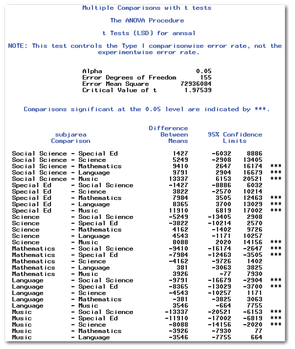
Figure 9.10 shows the subjarea comparisons twice. As an example, the comparison between science and special ed appears both as Science - Special Ed and as Special Ed - Science. The statistical significance is the same for both comparisons.
Figure 9.10 contains a note reminding you that this test controls the comparisonwise error rate. The output gives you additional information about the tests that were performed.
Understanding Other Items in the Report
Figure 9.10 contains two reports. The first report is the Information report, which contains the statistical details for the tests. The second report is the Pairs report, which contains the results of the pairwise comparisons.
The heading for both reports is t Tests (LSD) for annsal. For your data, the heading will contain the measurement-variable that you specify in the MODEL statement.
The LSD abbreviation in the heading appears because performing multiple t-tests when all group sizes are equal is the same as using a test known as Fisher’s Least Significant Difference test. This test is usually referred to as Fisher’s LSD test. You don’t need to worry about whether your sample sizes are equal or not. If you request multiple pairwise t-tests, SAS performs Fisher’s LSD test if it can be used.
The list below summarizes items in the Information report:
Alpha
is the α-level for the test. SAS automatically uses 0.05.
Error Degrees of Freedom
is the same as the degrees of freedom for Mean Square for Error in the ANOVA table.
Error Mean Square
is the same as the Mean Square for Error in the ANOVA table.
Critical Value of t
is the critical value for the tests. If the test statistic is greater than the critical value, the difference between the means of two groups is significant at the level given by Alpha.
The Pairs report also contains a column that identifies the comparison. For your data, the column heading will contain the measurement-variable. The report contains a column for Difference Between Means, which shows the difference between the two group averages in the row.
Technical Details: Overall Risk
When you perform multiple comparison procedures that control the comparisonwise error rate, you control the risk of making a wrong decision about each comparison. Here, the word “wrong” means concluding that groups are significantly different when they are not.
Controlling the comparisonwise error rate at 0.05 might give you a false sense of security. The more comparison-wise tests you perform, the higher your overall risk of making a wrong decision.
The salary data has 15 two-way comparisons for the 6 groups. Here is the overall risk of making a wrong decision:
1 - (0.95)15 = 0.537
This means that there is about a 54% chance of incorrectly concluding that two means are different in the salary data when the multiple pairwise t-tests are used. Most statisticians agree that this overall risk is too high to be acceptable.
In general, here is the overall risk:
1 - (0.95)m
m is the number of pairwise comparisons to be performed. These formulas assume that you perform each test at the 95% confidence level, which controls the comparisonwise error rate at 0.05. You can apply this formula to your own data to help you understand the overall risk of making a wrong decision.
The Bonferroni approach and the Tukey-Kramer test are two solutions for controlling the experimentwise error rate.
To control the experimentwise error rate with multiple pairwise t-tests, you can use the Bonferroni approach. With the Bonferroni approach, you decrease the alpha level for each test so that the overall risk of incorrectly concluding that the means are different is 5%. Basically, each test is performed using a very low alpha level. If you have many groups, the Bonferroni approach can be very conservative and can fail to detect significant differences between groups.
For the salary data, you want to control the experimentwise error rate at 0.05. There are 15 two-way comparisons. Essentially, performing each test to compare two means results in the following:
α= 0.05 / 15 = 0.0033
To use the Bonferroni approach, use the BON option in the MEANS statement in PROC ANOVA:
proc anova data=salary;
class subjarea;
model annsal=subjarea;
means subjarea / bon;
title 'Multiple Comparisons with Bonferroni Approach';
run;
These statements produce the results shown in Figures 9.5 and 9.6. Figure 9.11 shows the results for the multiple comparisons using the Bonferroni approach (produced by the BON option).
Deciding Which Means Differ
Figure 9.11 is very similar to Figure 9.10. It shows a 95% confidence interval for the difference between each pair of means.
SAS highlights comparisons that are significant with three asterisks (***) in the right-most column. From these results, you can conclude the following:
- The mean annual salary for Social Science is significantly different from Music.
- The mean annual salary for Special Ed is significantly different from Mathematics, Language, and Music.
- The mean annual salaries for other pairs of subject areas are not significantly different.
Compare the Bonferroni conclusions with the conclusions from the multiple pairwise t-tests. When controlling the experimentwise error rate, you find fewer significant differences between groups. However, you decrease your risk of incorrectly concluding that the means are different from each other.
In contrast, the results from the multiple pairwise t-tests detect more significant differences between groups. You have an increased overall risk of making incorrect decisions. Although you know that each comparison has an alpha level of 0.05, you don’t know the alpha level for the overall experiment.
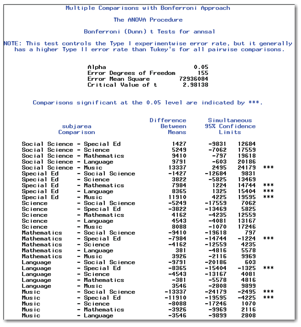
Understanding Other Items in the Report
Figure 9.11 contains two reports. Both are very similar to the reports in Figure 9.10. The first report is the Information report, which contains the statistical details for the tests. The second report is the Pairs report, which contains the results of the pairwise comparisons. See the information for Figure 9.10 for details on items in Figure 9.11.
The Critical Value of t in Figure 9.11 is higher than it is in Figure 9.10. This is a result of the lower per-comparison alpha level for the tests.
The heading for the reports in Figure 9.11 identifies the alternate name “Dunn” for the Bonferroni tests. The note below this heading refers to the Tukey-Kramer test, which is discussed in the next section. This note explains that the Bonferroni approach controls the experimentwise error rate.
Performing the Tukey-Kramer Test
The Tukey-Kramer test controls the experimentwise error rate. Many statisticians prefer this test to using the Bonferroni approach. This test is sometimes called the HSD test, or the honestly significant difference test in the case of equal group sizes.
To perform the Tukey-Kramer test, use the TUKEY option in the MEANS statement in PROC ANOVA:
proc anova data=salary;
class subjarea;
model annsal=subjarea;
means subjarea / tukey;
title 'Multiple Comparisons with Tukey-Kramer Test';
run;
These statements produce the results shown in Figures 9.5 and 9.6. Figure 9.12 shows the results for the multiple comparisons using the Tukey-Kramer test (produced by the TUKEY option).
The heading for the reports in Figure 9.12 identifies the test. The note below this heading explains that the Tukey-Kramer test controls the experimentwise error rate.

Deciding Which Means Differ
Figure 9.12 is very similar to Figure 9.10 and Figure 9.11. It shows a 95% confidence interval for the difference between each pair of means.
SAS highlights comparisons that are significant with three asterisks (***) in the right-most column. From these results, you can conclude the following:
- The mean annual salary for Social Science is significantly different from Music.
- The mean annual salary for Special Ed is significantly different from Mathematics, Language, and Music.
- The mean annual salaries for other pairs of subject areas are not significantly different.
These results are the same as the Bonferroni results, which makes sense because both tests control the experimentwise error rate. For your data, however, you might not get the exact same results from these two tests.
Understanding Other Items in the Report
Figure 9.12 contains two reports. Both are very similar to the reports in Figure 9.10 and Figure 9.11. The first report is the Information report, which contains the statistical details for the tests. The second report is the Pairs report, which contains the results of the pairwise comparisons. See the information for Figure 9.10 for details on items in Figure 9.12.
The Critical Value of Studentized Range in Figure 9.12 identifies the test statistic for the Tukey-Kramer test.
SAS automatically performs multiple comparison procedures and creates confidence intervals at the 95% confidence level. You can change the confidence level for any of the multiple comparison procedures with the ALPHA= option in the MEANS statement:
proc anova data=salary;
class subjarea;
model annsal=subjarea;
means subjarea / tukey alpha=0.10;
title 'Tukey-Kramer Test at 90%';
run;
These statements produce the results shown in Figures 9.5 and 9.6. Figure 9.13 shows the results for the multiple comparisons using the Tukey-Kramer test with a 0.10 alpha level (produced by the TUKEY and ALPHA= options).

Figure 9.13 is very similar to Figure 9.12. The key differences in appearance are the Alpha value in the Information report, and the column heading that indicates Simultaneous 90% Confidence Limits in the Pairs report.
Deciding Which Means Differ
SAS highlights comparisons that are significant with three asterisks (***) in the right-most column. From these results, you can conclude the following:
- The mean annual salaries for Social Science and Special Ed are significantly different from Mathematics, Language, and Music.
- The mean annual salary for Science is significantly different from Music.
- The mean annual salaries for other pairs of subject areas are not significantly different.
Because you used a lower confidence level (90% instead of 95%), it makes sense that you find more significant differences between groups.
Using Dunnett’s Test When Appropriate
Some experiments have a control group. For example, clinical trials to investigate the effectiveness of a new drug often include a placebo group, where the patients receive a look-alike pill. The placebo group is the control group. Dunnett’s test is designed for this situation. For example purposes only, assume that Mathematics is the control group for the salary data:
proc anova data=salary;
class subjarea;
model annsal=subjarea;
means subjarea / dunnett('Mathematics'),
title 'Means Comparisons with Mathematics as Control';
run;
The DUNNETT option performs the test. For your data, provide the value of the control group in parentheses. These statements produce the results shown in Figures 9.5 and 9.6. Figure 9.14 shows the results for the multiple comparisons using Dunnett’s test.
Figure 9.14 contains the Information report and the Pairs report. The heading for the reports identifies the test. The note below this heading explains that Dunnett’s test controls the experimentwise error rate in the situation of comparing all groups against a control group.

Deciding Which Means Differ
SAS highlights comparisons that are significant with three asterisks (***) in the right-most column. From these results, you can conclude the following:
- The mean annual salaries for Social Science and Special Ed are significantly different from Mathematics.
- The mean annual salaries for other subject areas are not significantly different from the control group of Mathematics.
Understanding Other Items in the Report
Figure 9.14 contains two reports. Both are very similar to the reports in Figure 9.10. The first report is the Information report, which contains the statistical details for the tests. The second report is the Pairs report, which contains the results of the pairwise comparisons. See the information for Figure 9.10 for details on items in Figure 9.14.
The Critical Value of Dunnett’s t in Figure 9.14 identifies the test statistic for Dunnett’s test.
First, use a multiple comparison test only after an analysis of variance is significant. If the ANOVA indicates that the means are not significantly different, then multiple comparison procedures are not appropriate. All of the multiple comparison procedures are available as options in the MEANS statement.
If you are interested in comparing all pairwise comparisons, and you want to control only the comparisonwise error rate, you can use the multiple pairwise t-tests with the T option.
If you have a few pre-planned comparisons between groups, and you want to control the experimentwise error rate, you can use the Bonferroni approach with the BON option.
If you want to compare all of the means between groups, and you want to control the experimentwise error rate, use either the Tukey-Kramer test or the Bonferroni approach. The Bonferroni approach is more conservative, and many statisticians prefer the Tukey-Kramer test. Use the TUKEY option for the Tukey-Kramer test.
If you have the special case of a known control group, you can use Dunnett’s test with the DUNNETT option.
Summarizing Multiple Comparison Procedures
SAS automatically displays results from multiple comparison procedures using confidence intervals when the data is unbalanced. The confidence intervals help you understand how much the group means differ. Confidence intervals also help you to assess the practical significance of the differences between groups. You can specify confidence intervals with the CLDIFF option.
SAS automatically uses connecting letters when the data is balanced, as shown in the next section. You can specify connecting letters with the LINES option. Consult with a statistician before using the LINES option with unbalanced data because differences in group sizes can mean that the approach is not appropriate.
The general form of the statements to perform multiple comparison procedures using PROC ANOVA is shown below:
PROC ANOVA DATA=data-set-name;
CLASS class-variable;
MODEL measurement-variable=class-variable;
MEANS class-variable / options;
The PROC ANOVA, CLASS, and MODEL statements are required.
The MEANS statement options can be one or more of the following:
T
multiple pairwise t-tests for pairwise comparisons.
BON
Bonferroni approach for multiple pairwise t-tests.
TUKEY
Tukey-Kramer test.
DUNNETT(‘control ’)
Dunnett’s test, where ‘control ’ identifies the control group. If you use formats in the data set, then use the formatted value in this option.
ALPHA=level
controls the significance level. Choose a level between 0.0001 and 0.9999. SAS automatically uses 0.05.
CLDIFF
shows differences with confidence intervals. SAS automatically uses confidence intervals for unequal group sizes.
LINES
shows differences with connecting letters. SAS automatically uses connecting letters for equal group sizes.
If any option is used, then the slash is required. You can use the options alone or together, as shown above.
PROC ANOVA has options for many other multiple comparison procedures. See the SAS documentation or the references in Appendix 1, “Further Reading,” for information.
Other items were defined earlier.
As discussed in Chapter 4, you can use the ODS statement to choose the output tables to display. Table 9.4 identifies the output tables for PROC ANOVA and multiple comparison procedures.
Using PROC ANOVA Interactively
PROC ANOVA is an interactive procedure. If you use line mode or the windowing environment mode, you can perform an analysis of variance, and then perform multiple comparison procedures without rerunning the analysis of variance. Type the PROC ANOVA, CLASS, and MODEL statements, and then add a RUN statement to see the analysis of variance. Then, add a MEANS statement, and a second RUN statement to perform multiple comparison procedures. These statements produce the results shown in Figures 9.5, 9.6, and 9.10:
proc anova data=salary;
class subjarea;
model annsal=subjarea;
title 'ANOVA for Teacher Salary Data';
run;
means subjarea / t;
title 'Multiple Comparisons with t Tests';
run;
quit;
When you use the statements above, the second RUN statement does not end PROC ANOVA because the procedure is waiting to receive additional statements. The QUIT statement ends the procedure. The form of the QUIT statement is simply the word QUIT followed by a semicolon.
Although you can end the procedure by starting another DATA or PROC step, you might receive an error. If you use an ODS statement before the next PROC step, and the table you specify in the ODS statement is not available in PROC ANOVA (which is running interactively), SAS prints an error in the log and does not create output. To avoid this situation, use the QUIT statement.
This section summarizes the steps for performing the analyses to compare multiple groups. This data has equal group sizes, so it is balanced.
Step 1: Create a SAS data set.
The data is from an experiment that compares muzzle velocities for different types of gunpowder. The muzzle velocity is measured for eight cartridges from each of the three types of gunpowder. Table 9.5 shows the data.

This data is available in the bullets data set in the sample data for the book. The following SAS statements create the data set:
data bullets;
input powder $ velocity @@;
datalines;
BLASTO 27.3 BLASTO 28.1 BLASTO 27.4 BLASTO 27.7
BLASTO 28.0 BLASTO 28.1 BLASTO 27.4 BLASTO 27.1
ZOOM 28.3 ZOOM 27.9 ZOOM 28.1 ZOOM 28.3 ZOOM 27.9
ZOOM 27.6 ZOOM 28.5 ZOOM 27.9 KINGPOW 28.4 KINGPOW 28.9 KINGPOW 28.3 KINGPOW 27.9 KINGPOW 28.2 KINGPOW 28.9
KINGPOW 28.8 KINGPOW 27.7
;
run;
Step 2: Check the data set for errors.
Following similar steps as you did for the salary data, use PROC MEANS and PROC BOXPLOT to summarize the data and check it for errors:
proc means data=bullets;
class powder;
var velocity;
title 'Brief Summary of Bullets Data';
run;
proc boxplot data=bullets;
plot velocity*powder / boxwidthscale=1 bwslegend;
title 'Comparative Box Plots by Gunpowder';
run;
Figures 9.15 and 9.16 show the results.
From the statistics and the box plots, you initially conclude that KINGPOW has a higher mean velocity than the other two types of gunpowder. But, you don’t know whether this observed difference is statistically significant. Because the three groups are the same size, the box widths are all the same. Because PROC BOXPLOT does not scale the box widths, the graph does not contain a legend.
The box plots don’t reveal any outlier points or potential errors in the data. Proceed with the analysis.

Step 3: Choose the significance level for the test.
Test for differences between the three groups of gunpowder using the 5% significance level. The reference value is 0.05.

Step 4: Check the assumptions for the test.
In checking the assumptions for an analysis of variance, note that the observations are independent. The standard deviations for the three groups are similar. With only eight observations per group, it is difficult to test for normality. For completeness, to check these assumptions, type the following:
ods select HOVFTest;
proc anova data=bullets;
class powder;
model velocity=powder;
means powder / hovtest;
title 'Testing Equal Variances for Bullets Data';
run;
quit;
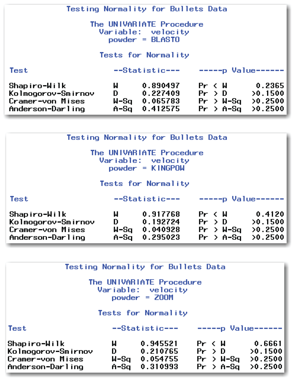
ods select TestsForNormality;
proc univariate data=bullets normal;
class powder;
var velocity;
title 'Testing Normality for Bullets Data';
run;
Figure 9.17 shows the results from testing for equal variances. Proceed with the analysis based on the assumption that the variances for the three groups are the same.
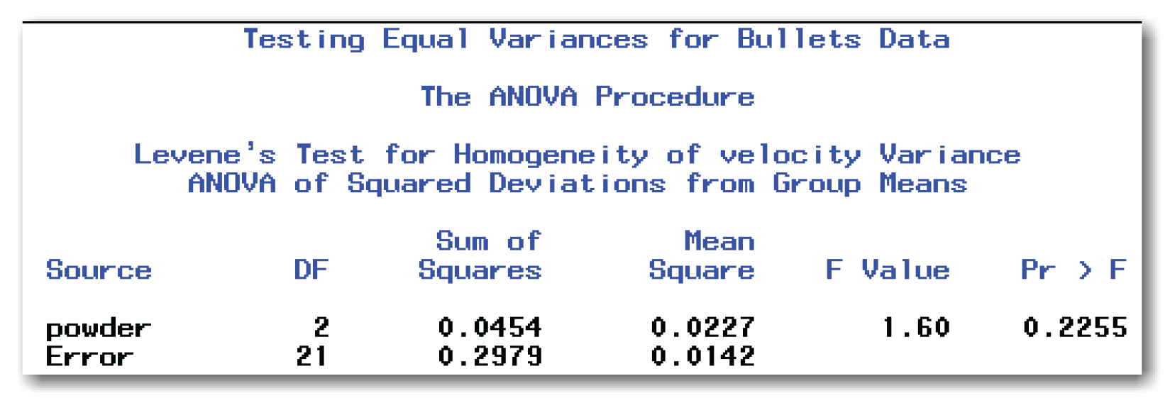
Figure 9.18 shows the resulting text reports from testing for normality in each group. Even though the sample sizes are small, these results indicate that you can assume normality and proceed with the analysis. For completeness, you might want to perform informal checks using histograms, normal probability plots, skewness, and kurtosis. These informal checks can be difficult with such small groups, so this chapter does not show them.
Step 5: Perform the test.
Use PROC ANOVA to perform an analysis of variance. For example purposes only, this step also shows the results of the Kruskal-Wallis test.
proc anova data=bullets;
class powder;
model velocity=powder;
means powder / hovtest;
title 'ANOVA for Bullets Data';
run;
quit;
proc npar1way data=bullets wilcoxon;
class powder;
var velocity;
title 'Nonparametric Tests for Bullets Data';
run;
Figure 9.19 shows the results from the analysis of variance. Figure 9.20 shows the results from the Kruskal-Wallis test. PROC ANOVA prints a first page that shows the CLASS variable, the levels of the CLASS variable, and the values. It also shows the number of observations for the analysis. This first page is similar to the first page shown for the salary data in Figure 9.5.


Step 6: Make conclusions from the test results.
The p-value for comparing groups is 0.0033, which is less than the reference probability value of 0.05. You conclude that the mean velocity is significantly different between the three types of gunpowder. If the analysis of variance assumptions had not seemed reasonable, then the Kruskal-Wallis test would have led to the same conclusion, with p=0.0131.
Next, perform the Tukey-Kramer test. Use the following MEANS statement:
means powder / tukey;
title 'Tukey Kramer Test for Bullets Data';
run;
Figure 9.21 shows the results. The note for the test refers to another multiple comparison test, REGWQ, which is not discussed in this book. Compare Figures 9.21 and 9.12. When PROC ANOVA shows the results of the Tukey-Kramer test using confidence intervals, the heading for the test is slightly different from when the procedure shows the results using connecting lines.
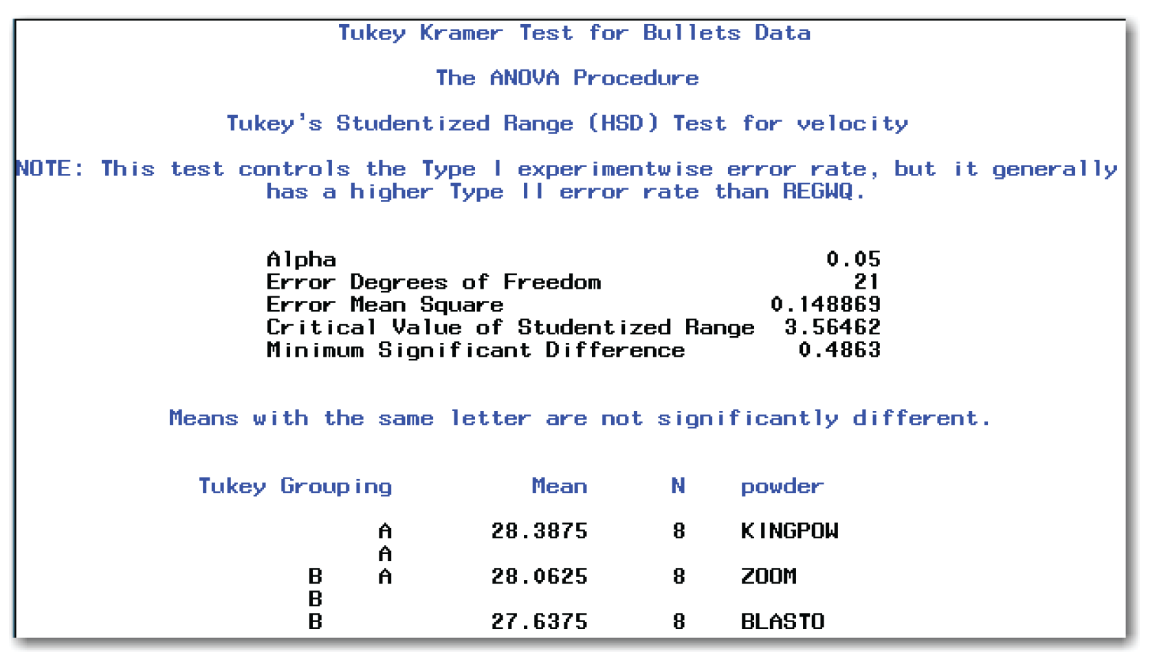
You conclude that the mean muzzle velocity for KINGPOW is significantly different from BLASTO. The mean muzzle velocities for other pairs of types of gunpowder are not significantly different. These conclusions should make sense at an intuitive level when you look at the side-by-side box plots from PROC UNIVARIATE. However, now you know that the differences between groups are greater than could be expected by chance. Without the statistical test, you only knew that the groups seemed different, but you didn’t know how likely the observed differences were.
- To summarize data from more than two groups, separate the data into groups, and get summary information for each group using one or more SAS procedures. See “Syntax” for more detail.
- The steps for analyses are:
1. Create a SAS data set.
2. Check the data set for errors.
3. Choose the significance level for the test.
4. Check the assumptions for the test.
5. Perform the test.
6. Make conclusions from the test results.
- An analysis of variance (ANOVA) is a test for comparing the means of multiple groups at once. This test assumes that the observations are independent random samples from normally distributed populations, and that the groups have equal variances.
- The Welch’s ANOVA compares the means of multiple groups when the assumption of equal variances does not seem reasonable.
- If the normality assumption does not seem reasonable, the Kruskal-Wallis test provides a nonparametric analogue.
- Compare the p-value for the test with the significance level.
- If the p-value is less than the significance level, then reject the null hypothesis. Conclude that the means for the groups are significantly different.
- If the p-value is greater than the significance level, then you fail to reject the null hypothesis. Conclude that the means for the groups are not significantly different. Do not conclude that the means for the groups are the same.
- Multiple comparisons tests show which means differ from other means. Use multiple comparison procedures only after an analysis of variance shows significant differences between groups. Multiple pairwise t-tests control the comparisonwise error rate, but increase the overall risk of incorrectly concluding that the means are different. The Tukey-Kramer test and Bonferroni approach control the experimentwise error rate. Dunnett’s test is useful in the special case of a known control group.
To summarize data from multiple groups
- To create a concise summary of multiple groups, use PROC MEANS with a CLASS statement.
- To create a detailed summary of multiple groups, use PROC UNIVARIATE with a CLASS statement. This summary contains output tables for each value of the class-variable. You can use the PLOT option to create line printer plots for each value of the class-variable.
- To create a detailed summary of multiple groups with comparative histograms:
PROC UNIVARIATE DATA=data-set-name NOPRINT;
CLASS class-variable;
VAR measurement-variables;
HISTOGRAM measurement-variables / NROWS=value;
data-set-name
is the name of a SAS data set.
class-variable
is the variable that classifies the data into groups.
measurement-variables
are the variables you want to summarize.
The CLASS statement is required. The class-variable can be character or numeric and should be nominal. If you omit the measurement-variables from the VAR statement, then the procedure uses all numeric variables.
You can use the options described in Chapters 4 and 5 with PROC UNIVARIATE and a CLASS statement. You can omit the NOPRINT option and create the detailed summary and histograms at the same time.
The NROWS= option controls the number of histograms that appear on a single page. SAS automatically uses NROWS=2. For your data, choose a value equal to the number of groups.
If any option is used in the HISTOGRAM statement, then the slash is required.
- To create a detailed summary of multiple groups with side-by-side bar charts, use PROC CHART. This is a low-resolution alternative to comparative histograms.
- To create side-by-side box plots:
PROC BOXPLOT DATA=data-set-name;
PLOT measurement-variable*class-variable
/ BOXWIDTHSCALE=1 BWSLEGEND;
Items in italic were defined earlier in the chapter. Depending on your data, you might need to first sort by the class-variable before creating the plots. The asterisk in the PLOT statement is required.
The BOXWIDTHSCALE=1 option scales the width of the box based on the sample size of each group. The BWSLEGEND option adds a legend to the bottom of the box plot. The legend explains the varying box widths. If either option is used, then the slash is required. You can use the options alone or together, as shown above.
To check the assumptions (step 4)
- To check the assumption of independent observations, you need to think about your data and whether this assumption seems reasonable. This is not a step where using SAS will answer this question.
- To check the assumption of normality, use PROC UNIVARIATE. For multiple groups, check each group separately.
- To test the assumption of equal variances:
PROC ANOVA DATA=data-set-name;
CLASS class-variable;
MODEL measurement-variable=class-variable;
MEANS class-variable / HOVTEST;
Items in italic were defined earlier in the chapter.
The PROC ANOVA, CLASS, and MODEL statements are required.
To perform the test (step 5)
- If the analysis of variance assumptions seem reasonable:
PROC ANOVA DATA=data-set-name;
CLASS class-variable;
MODEL measurement-variable=class-variable;
Items in italic were defined earlier in the chapter.
The PROC ANOVA, CLASS, and MODEL statements are required.
- If the equal variances assumption does not seem reasonable:
PROC ANOVA DATA=data-set-name;
CLASS class-variable;
MODEL measurement-variable=class-variable;
MEANS class-variable / WELCH;
Items in italic were defined earlier in the chapter.
The PROC ANOVA, CLASS, and MODEL statements are required.
If the Welch ANOVA is used, then multiple comparison procedures are not appropriate.
- If you use PROC ANOVA interactively in the windowing environment mode, then end the procedure with the QUIT statement:
QUIT;
- For non-normal data:
PROC NPAR1WAY DATA=data-set-name WILCOXON;
CLASS class-variable;
VAR measurement-variables;
Items in italic were defined earlier in the chapter.
The CLASS statement is required.
While the VAR statement is not required, you should use it. If you omit the VAR statement, then PROC NPAR1WAY performs analyses for every numeric variable in the data set.
For performing multiple comparison procedures
- First, compare groups and perform multiple comparison procedures only when you conclude that the groups are significantly different.
PROC ANOVA DATA=data-set-name;
CLASS class-variable;
MODEL measurement-variable=class-variable;
MEANS class-variable / options;
Other items were defined earlier.
The PROC ANOVA, CLASS, and MODEL statements are required.
The MEANS statement options can be one or more of the following:
T
multiple pairwise t-tests for pairwise comparisons.
BON
Bonferroni approach for multiple pairwise t-tests.
TUKEY
Tukey-Kramer test.
DUNNETT(‘control ’)
Dunnett’s test, where ‘control ’ identifies the control group. If you use formats in the data set, then use the formatted value in this option.
ALPHA=level
controls the significance level. Choose a level between 0.0001 and 0.9999. SAS automatically uses 0.05.
CLDIFF
shows differences with confidence intervals. SAS automatically uses confidence intervals for unequal group sizes.
LINES
shows differences with connecting letters. SAS automatically uses connecting letters for equal group sizes.
If any option is used, then the slash is required. You can use the options alone or together.
PROC ANOVA has options for many other multiple comparison procedures. See the SAS documentation or the references in Appendix 1, “Further Reading,” for information.
The program below produces the output shown in this chapter:
options nodate nonumber ps=60 ls=80;
proc format;
value $subtxt
'speced' = 'Special Ed'
'mathem' = 'Mathematics'
'langua' = 'Language'
'music' = 'Music'
'scienc' = 'Science'
'socsci' = 'Social Science';
run;
data salary;
input subjarea $ annsal @@;
label subjarea='Subject Area'
annsal='Annual Salary';
format subjarea $subtxt.;
datalines;
speced 35584 mathem 27814 langua 26162 mathem 25470
speced 41400 mathem 34432 music 21827 music 35787 music 30043
mathem 45480 mathem 25358 speced 42360 langua 23963 langua 27403
mathem 29610 music 27847 mathem 25000 mathem 29363 mathem 25091
speced 31319 music 24150 langua 30180 socsci 42210 mathem 55600
langua 32134 speced 57880 mathem 47770 langua 33472 music 21635
mathem 31908 speced 43128 mathem 33000 music 46691 langua 28535
langua 34609 music 24895 speced 42222 speced 39676 music 22515
speced 41899 music 27827 scienc 44324 scienc 43075 langua 49100
langua 44207 music 46001 music 25666 scienc 30000 mathem 26355
mathem 39201 mathem 32000 langua 26705 mathem 37120 langua 44888
mathem 62655 scienc 24532 mathem 36733 langua 29969 mathem 28521
langua 27599 music 27178 mathem 26674 langua 28662 music 41161
mathem 48836 mathem 25096 langua 27664 music 23092 speced 45773
mathem 27038 mathem 27197 music 44444 speced 51096 mathem 25125
scienc 34930 speced 44625 mathem 27829 mathem 28935 mathem 31124
socsci 36133 music 28004 mathem 37323 music 32040 scienc 39784
mathem 26428 mathem 39908 mathem 34692 music 26417 mathem 23663
speced 35762 langua 29612 scienc 32576 mathem 32188 mathem 33957
speced 35083 langua 47316 mathem 34055 langua 27556 langua 35465
socsci 49683 langua 38250 langua 30171 mathem 53282 langua 32022
socsci 31993 speced 52616 langua 33884 music 41220 mathem 43890
scienc 40330 langua 36980 scienc 59910 mathem 26000 langua 29594
socsci 38728 langua 47902 langua 38948 langua 33042 mathem 29360
socsci 46969 speced 39697 mathem 31624 langua 30230 music 29954
mathem 45733 music 24712 langua 33618 langua 29485 mathem 28709
music 24720 mathem 51655 mathem 32960 mathem 45268 langua 31006
langua 48411 socsci 59704 music 22148 mathem 27107 scienc 47475
langua 33058 speced 53813 music 38914 langua 49881 langua 42485
langua 26966 mathem 31615 mathem 24032 langua 27878 mathem 56070
mathem 24530 mathem 40174 langua 27607 speced 31114 langua 30665
scienc 25276 speced 36844 mathem 24305 mathem 35560 music 28770
langua 34001 mathem 35955
;
run;
proc means data=salary;
class subjarea
var annsal;
title 'Brief Summary of Teacher Salaries';
run;
proc univariate data=salary noprint;
class subjarea;
var annsal;
histogram annsal / nrows=6;
title 'Comparative Histograms by Subject Area';
run;
proc sort data=salary;
by subjarea;
run;
proc boxplot data=salary;
plot annsal*subjarea / boxwidthscale=1 bwslegend;
title 'Comparative Box Plots by Subject Area';
run;
proc anova data=salary;
class subjarea;
model annsal=subjarea;
title 'ANOVA for Teacher Salaries';
run;
quit;
ods select means HOVFtest;
proc anova data=salary;
class subjarea;
model annsal=subjarea;
means subjarea / hovtest;
title 'Testing for Equal Variances';
run;
quit;
ods select Welch;
proc anova data=salary;
class subjarea;
model annsal=subjarea;
means subjarea / welch;
title 'Welch ANOVA for Salary Data';
run;
proc npar1way data=salary wilcoxon;
class subjarea;
var annsal;
title 'Nonparametric Tests for Teacher Salaries' ;
run;
proc anova data=salary;
class subjarea;
model annsal=subjarea;
means subjarea / t;
title 'Multiple Comparisons with t tests';
run;
means subjarea / bon ;
title 'Multiple Comparisons with Bonferroni Approach' ;
run;
means subjarea / tukey;
title 'Means Comparisons with Tukey-Kramer Test';
run;
means subjarea / tukey alpha=0.10 ;
title 'Tukey-Kramer Test at 90%';
run;
means subjarea / dunnett('Mathematics') ;
title 'Means Comparisons with Mathematics as Control';
run;
data bullets;
input powder $ velocity @@;
datalines;
BLASTO 27.3 BLASTO 28.1 BLASTO 27.4 BLASTO 27.7 BLASTO 28.0
BLASTO 28.1 BLASTO 27.4 BLASTO 27.1 ZOOM 28.3 ZOOM 27.9
ZOOM 28.1 ZOOM 28.3 ZOOM 27.9 ZOOM 27.6 ZOOM 28.5 ZOOM 27.9
KINGPOW 28.4 KINGPOW 28.9 KINGPOW 28.3 KINGPOW 27.9
KINGPOW 28.2 KINGPOW 28.9 KINGPOW 28.8 KINGPOW 27.7
;
run;
proc means data=bullets;
class powder;
var velocity;
title 'Brief Summary of Bullets Data';
run;
proc boxplot data=bullets;
plot velocity*powder / boxwidthscale=1 bwslegend;
title 'Comparative Box Plots by Gunpowder';
run;
ods select HOVFtest;
proc anova data=bullets;
class powder;
model velocity=powder;
means powder / hovtest;
title 'Testing Equal Variances for Bullets Data';
run;
quit;
ods select TestsForNormality;
proc univariate data=bullets normal;
class powder;
var velocity;
title 'Testing Normality for Bullets Data';
run;
proc anova data=bullets;
class powder;
model velocity=powder;
title 'ANOVA for Bullets Data';
run;
means powder / tukey;
title 'Tukey Kramer Test for Bullets Data';
run;
quit;
proc npar1way data=bullets wilcoxon;
class powder;
var velocity;
title 'Nonparametric Tests for Bullets Data' ;
run;
ENDNOTE
[1] Data is from Dr. Ramon Littell, University of Florida. Used with permission.