Chapter 8 Comparing Two Independent Groups
Do male accountants earn different salaries than female accountants? Do people who are given a new shampoo use a different amount of shampoo than people who are given an old shampoo? Do cows that are fed a grain supplement and hay gain a different amount of weight than cows that are fed only hay?
These questions involve comparing two independent groups of data (as defined in the previous chapter). The variable that classifies the data into two groups should be nominal. The response variable can be ordinal or continuous, but must be numeric. This chapter discusses the following topics:
- summarizing data from two independent groups
- building a statistical test of hypothesis to compare the two groups
- deciding which statistical test to use
- performing statistical tests for independent groups
For the various tests, this chapter shows how to use SAS to perform the test, and how to interpret the test results.
Deciding between Independent and Paired Groups
Using PROC MEANS for a Concise Summary
Using PROC UNIVARIATE for a Detailed Summary
Adding Comparative Histograms to PROC UNIVARIATE
Using PROC CHART for Side-by-Side Bar Charts
Using PROC BOXPLOT for Side-by-Side Box Plots
Building Hypothesis Tests to Compare Two Independent Groups
Deciding Which Statistical Test to Use
Performing the Two-Sample t-test
Changing the Alpha Level for Confidence Intervals
Performing the Wilcoxon Rank Sum Test
Using PROC NPAR1WAY for the Wilcoxon Rank Sum Test
Deciding between Independent and Paired Groups
When comparing two groups, you want to know whether the means for the two groups are different. The first step is to decide whether you have independent or paired groups. See Chapter 7 for more detail on this decision.
This section explains how to summarize data from two independent groups. These methods provide additional understanding of the statistical results.
Table 8.1 shows the percentages of body fat for several men and women. These people participated in unsupervised aerobic exercise or weight training (or both) about three times per week for a year. Then, they were measured once at the end of the year. Chapter 1 introduced this data, and Chapter 4 summarized the frequency counts for men and women in the fitness program.
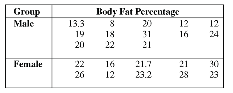
This data is available in the bodyfat data set in the sample data for the book.
The next five topics discuss methods for summarizing this data.
Using PROC MEANS for a Concise Summary
Just as you can use PROC MEANS for a concise summary of one variable, you can use the procedure for a concise summary of two independent groups. You add the CLASS statement to identify the variable that classifies the data into groups. The SAS statements below create the data set and provide a brief summary of the body fat percentages for men and women.
proc format;
value $gentext 'm' = 'Male'
'f' = 'Female';
run;
data bodyfat;
input gender $ fatpct @@;
format gender $gentext.;
label fatpct='Body Fat Percentage';
datalines;
m 13.3 f 22 m 19 f 26 m 20 f 16 m 8 f 12 m 18 f 21.7
m 22 f 23.2 m 20 f 21 m 31 f 28 m 21 f 30 m 12 f 23
m 16 m 12 m 24
;
run;
proc means data=bodyfat;
class gender;
var fatpct;
title 'Brief Summary of Groups';
run;
Figure 8.1 shows the results.
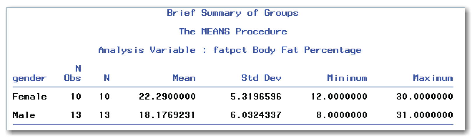
Figure 8.1 shows descriptive statistics for each gender. The column labeled gender identifies the levels of the CLASS variable, and the other columns provide descriptive statistics. For example, the average percentage of body fat for women is 22.29. The average percentage of body fat for men is 18.18. The standard deviation for women is 5.32, and for men it is 6.03. The range of values for women is 12 to 30, and for men it is 8 to 31. If you plotted these values on a number line, you would see a wide range of overlapping values.
From this summary, you might initially conclude that the means for the two groups are different. You don’t know whether this difference is greater than what could happen by chance. Finding out whether the difference is due to chance or is real requires a statistical test. This statistical test is discussed in “Building Hypothesis Tests to Compare Two Independent Groups” later in this chapter.
The general form of the statements to create a concise summary of two independent groups using PROC MEANS is shown below:
PROC MEANS DATA=data-set-name;
CLASS class-variable;
VAR measurement-variables;
data-set-name is the name of a SAS data set, class-variable is a variable that classifies the data into groups, and measurement-variables are the variables that you want to summarize.
To compare two independent groups, the CLASS statement is required. The class-variable can be character or numeric and should be nominal. If you omit the measurement-variables from the VAR statement, then the procedure uses all numeric variables.
You can use the statistical-keywords described in Chapter 4 with PROC MEANS and a CLASS statement.
Using PROC UNIVARIATE for a Detailed Summary
Just as you can use PROC UNIVARIATE for a detailed summary of one variable, you can use the procedure for a detailed summary of two independent groups. You add the CLASS statement to identify the variable that classifies the data into groups. The SAS statements below provide a detailed summary of the body fat percentages for men and women.
ods select moments basicmeasures extremeobs plots;
proc univariate data=bodyfat plot;
class gender;
var fatpct;
title 'Detailed Summary of Groups';
run;
The ODS statement controls the tables displayed in the output. Figure 8.2 shows the results.
Figure 8.2 shows descriptive statistics for each gender. For each of the tables that PROC UNIVARIATE creates, the output shows the statistics for each level of the CLASS variable. For example, look at the Basic Statistical Measures tables. The gender=Female table identifies statistics for women, and the gender=Male table identifies statistics for men.
Figure 8.2 shows a missing mode for the females. For data where no repetition of a value occurs, PROC UNIVARIATE does not print a mode. Table 8.1 shows the data, and you can see that each value of the body fat percentage is unique for the women. For the men, the values of 12 and 20 each occur twice. Figure 8.2 shows the mode for men as 12, and prints a note stating that this is the smallest of two modes in the data.
The PLOT option creates box plots, stem-and-leaf plots, and normal quantile plots for each gender. Figure 8.2 does not show the normal quantile plots. Chapter 4 discusses using these plots to check for errors in the data. Chapter 5 discusses how these plots are useful in checking the data for normality. You can visually compare the plots for the two groups. However, you might prefer comparative plots instead. See the next three topics for comparative histograms, comparative bar charts, and side-by-side box plots.
This more extensive PROC UNIVARIATE summary supports your initial thoughts that the means for the two groups are different. Finding out whether the difference is due to chance or is real requires a statistical test. This statistical test is discussed in “Building Hypothesis Tests to Compare Two Independent Groups” later in this chapter.
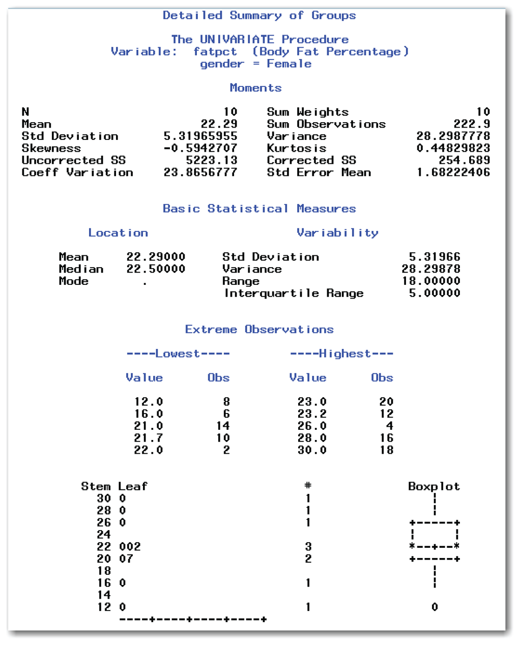
Figure 8.2 Detailed Summary of Two Independent Groups (continued)

The general form of the statements to create a detailed summary of two independent groups using PROC UNIVARIATE is shown below:
PROC UNIVARIATE DATA=data-set-name;
CLASS class-variable;
VAR measurement-variables;
Items in italic were defined earlier in the chapter.
To compare two independent groups, the CLASS statement is required. The class-variable can be character or numeric and should be nominal. If you omit the measurement-variables from the VAR statement, then the procedure uses all numeric variables.
You can use the options described in Chapters 4 and 5 with PROC UNIVARIATE and a CLASS statement.
Adding Comparative Histograms to PROC UNIVARIATE
Just as you can use PROC UNIVARIATE for a histogram of one variable, you can use the procedure for comparative histograms of two independent groups. You add the CLASS statement to identify the variable that classifies the data into groups. You also add the HISTOGRAM statement to request histograms. (To create high-resolution histograms, you must have SAS/GRAPH software licensed.) The SAS statements below provide comparative histograms. The NOPRINT option suppresses the printed output tables with the detailed summary of the body fat percentages for men and women.
proc univariate data=bodyfat noprint;
class gender;
var fatpct;
histogram fatpct;
title 'Comparative Histograms of Groups';
run;
Figure 8.3 shows the results.

The HISTOGRAM statement creates the pair of histograms in Figure 8.3. These histograms are plotted on the same axis scales. This approach helps you visually compare the distribution of the two groups.
The distribution of values for the men is more symmetrical and more spread out. It has more values at the lower end of the range. These graphs support your initial thoughts that the means for the two groups are different.
The general form of the statements to create comparative histograms of two independent groups using PROC UNIVARIATE is shown below:
PROC UNIVARIATE DATA=data-set-name NOPRINT;
CLASS class-variable;
VAR measurement-variables;
HISTOGRAM measurement-variables;
Items in italic were defined earlier in the chapter. You can omit the NOPRINT option and create the detailed summary and histograms at the same time. If you omit the measurement-variables from the HISTOGRAM statement, then the procedure uses all numeric variables in the VAR statement. If you omit the measurement-variables from the HISTOGRAM and VAR statements, then the procedure uses all numeric variables. You cannot specify variables in the HISTOGRAM statement unless the variables are also specified in the VAR statement.
Using PROC CHART for Side-by-Side Bar Charts
Figure 8.2 shows the line printer stem-and-leaf plots separately for the men and women in the fitness program. Figure 8.3 shows high-resolution histograms for these two independent groups. If you do not have SAS/GRAPH software licensed, you can use PROC CHART to create side-by-side bar charts that are low resolution (line printer quality).
proc chart data=bodyfat;
vbar fatpct / group=gender;
title 'Charts for Fitness Program';
run;
You can list only one variable in the GROUP= option. This variable can be either character or numeric, and it should have a limited number of levels. Variables such as height, weight, and temperature are not appropriate variables for the GROUP= option because they have many levels. Producing a series of side-by-side bar charts with one observation in each bar does not summarize the data well.
PROC CHART arranges the levels of the grouping variable in increasing numeric or alphabetical order. It uses the same bar midpoints for each group.
Figure 8.4 shows the results.
These bar charts are similar to the histograms in that they help you visually compare the distribution of the two groups. Again, the distribution of values for the men is more spread out than for the women, and has more values at the lower end of the range. These graphs support your initial thoughts that the means for the two groups are different.
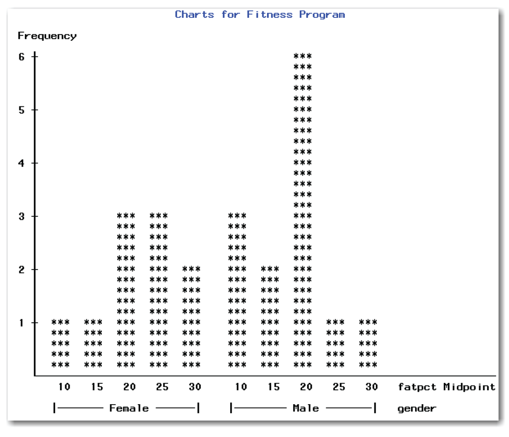
Compare Figures 8.3 and 8.4, which have different midpoints for the bars. In Figure 8.4, the symmetry of the distribution of values for the men is not as obvious as in Figure 8.3.
The general form of the statements to create comparative bar charts for two independent groups using PROC CHART is shown below:
PROC CHART DATA=data-set-name;
VBAR measurement-variables / GROUP=class-variable;
Items in italic were defined earlier in the chapter. For comparative horizontal bar charts, replace VBAR with HBAR.
Like other options in PROC CHART, the GROUP= option appears after the slash. You can use the GROUP= option with other PROC CHART options discussed in Chapter 4.
Although you can list only one variable in the GROUP= option, you can specify several measurement-variables to be charted, and you can produce several side-by-side bar charts simultaneously. If you list several measurement-variables before the slash, SAS creates side-by-side bar charts for each variable. Suppose you measure the calories, calcium content, and vitamin D content of several cartons of regular and skim milk. The variable that classifies the data into groups is milktype. Suppose you want side-by-side bar charts for each of the three measurement variables. In SAS, you type the statements below:
proc chart data=dairy;
vbar calories calcium vitamind / group=milktype;
run;
The statements produce three side-by-side bar charts, one for each of the measurement variables listed.
Using PROC BOXPLOT for Side-by-Side Box Plots
Figure 8.2 shows separate line printer box plots for the men and women in the fitness program. You can use PROC BOXPLOT to create high-resolution plots and display side-by-side box plots. (To create high-resolution box plots, you must have SAS/GRAPH software licensed.) The SAS statements below provide comparative box plots:
proc sort data=bodyfat;
by gender;
run;
proc boxplot data=bodyfat;
plot fatpct*gender;
title 'Comparative Box Plots of Groups';
run;
PROC BOXPLOT expects the data to be sorted by the variable that classifies the data into groups. If your data is already sorted, you can omit the PROC SORT step. The first variable in the PLOT statement identifies the measurement variable, and the second variable identifies the variable that classifies the data into groups. Figure 8.5 shows the results.

From the box plots, the distribution of values for males is wider than it is for females. You can also see this in the comparative histograms in Figure 8.3 and the bar charts in Figure 8.4. The box plots add the ability to display the mean, median, and interquartile range for each group. The lines at the ends of the whiskers are the minimum and maximum values for each group. Figure 8.5 shows the mean and median for males are lower than the mean and median for females. Figure 8.5 also shows the ends of the box for males (the 25th and 75th percentiles) are lower than the ends of the box for females. The box plots support your initial thoughts that the means for the two groups are different.
The general form of the statements to create side-by-side box plots for two independent groups using PROC BOXPLOT is shown below:
PROC BOXPLOT DATA=data-set-name;
PLOT measurement-variable*class-variable;
Items in italic were defined earlier in the chapter. Depending on your data, you might need to first sort by the class-variable before creating the plots. The asterisk in the PLOT statement is required.
Building Hypothesis Tests to Compare Two Independent Groups
So far, this chapter has discussed how to summarize differences between two independent groups. Suppose you want to know how important the differences are, and if the differences are large enough to be significant. In statistical terms, you want to perform a hypothesis test. This section discusses hypothesis testing when comparing two independent groups. (See Chapter 5 for the general idea of hypothesis testing.)
In building a test of hypothesis, you work with two hypotheses. When comparing two independent groups, the null hypothesis is that the two means for the independent groups are the same, and the alternative hypothesis is that the two means are different. In this case, the notation is the following:
Ho: μA = μB
Ha: μA ≠ μB
Ho indicates the null hypothesis, Ha indicates the alternative hypothesis, and μa and μB are the population means for independent groups A and B.
In statistical tests that compare two independent groups, the hypotheses are tested by calculating a test statistic from the data, and then comparing its value to a reference value that would be the result if the null hypothesis were true. The test statistic is compared to different reference values that are based on the sample size. In part, this is because smaller differences can be detected with larger sample sizes. As a result, if you use the reference value for a large sample size on a smaller sample, you are more likely to incorrectly conclude that the means for the groups are different when they are not.
This concept is similar to the concept of confidence intervals, in which different t-values are used (discussed in Chapter 6). With confidence intervals, the t-value is based on the degrees of freedom, which were determined by the sample size. Similarly, when comparing two independent groups, the degrees of freedom for a reference value are based on the sample sizes of the two groups. Specifically, the degrees of freedom are equal to N-2, where N is the total sample size for the two groups.
Deciding Which Statistical Test to Use
Because you test different hypotheses for independent and paired groups, you use different tests. In addition, there are parametric and nonparametric tests for each type of group. When deciding which statistical test to use, first, decide whether you have independent groups or paired groups.
Then, decide whether you should use a parametric or a nonparametric test. This second decision is based on whether the assumptions for the parametric test seem reasonable. In general, if the assumptions for the parametric test seem reasonable, use the parametric test. Although nonparametric tests have fewer assumptions, these tests typically are less powerful in detecting differences between groups.
The rest of this chapter describes the test to use for two independent groups. See Chapter 7 for details on the tests for the two situations for paired groups. Table 8.3 summarizes the tests.

The steps for performing the analyses to compare independent groups are the following:
1. Create a SAS data set.
2. Check the data set for errors.
3. Choose the significance level for the test.
4. Check the assumptions for the test.
5. Perform the test.
6. Make conclusions from the test results.
The rest of this chapter uses these steps for all analyses.
For each of the four tests in Table 8.3, there are two possible results: the p-value is less than the reference probability, or it is not. (See Chapter 5 for discussions on significance levels and on understanding practical significance and statistical significance.)
Groups Significantly Different
If the p-value is less than the reference probability, the result is statistically significant, and you reject the null hypothesis. For independent groups, you conclude that the means for the two groups are significantly different.
Groups Not Significantly Different
If the p-value is greater than the reference probability, the result is not statistically significant, and you fail to reject the null hypothesis. For independent groups, you conclude that the means for the two groups are not significantly different.
Do not conclude that the means for the two groups are the same. You do not have enough evidence to conclude that the means are the same. The results of the test indicate only that the means are not significantly different. You never have enough evidence to conclude that the population is exactly as described by the null hypothesis. In statistical hypothesis testing, do not accept the null hypothesis. Instead, either reject or fail to reject the null hypothesis. For a more detailed discussion of hypothesis testing, see Chapter 5.
Performing the Two-Sample t-test
The two-sample t-test is a parametric test for comparing two independent groups.
The three assumptions for the two-sample t-test are the following:
- observations are independent
- observations in each group are a random sample from a population with a normal distribution
- variances for the two independent groups are equal
Because of the second assumption, the two-sample t-test applies to continuous variables only.
Apply the six steps of analysis:
1. Create a SAS data set.
2. Check the data set for errors. Use PROC UNIVARIATE to check for errors. Based on the results, assume that the data is free of errors.
3. Choose the significance level for the test. Choose a 5% significance level, which requires a p-value less than 0.05 to conclude that the groups are significantly different.
4. Check the assumptions for the test.
The first assumption is independent observations. The assumption seems reasonable because each person’s body fat measurement is unrelated to every other person’s body fat measurement.
The second assumption is that the observations in each group are from a normal distribution. You can test this assumption for each group to determine whether this assumption seems reasonable. (See Chapter 6.)
The third assumption of equal variances seems reasonable based on the similarity of the standard deviations of the two groups. From Figure 8.2, the standard deviation is 5.32 for females and 6.03 for males. See “Testing for Equal Variances” for a statistical test to check this assumption.
5. Perform the test. PROC TTEST provides the exact two-sample t-test, which assumes equal variances, and an approximate test, which can be used if the assumption of equal variances isn’t met. See “Testing to Compare Two Means.”
6. Make conclusions from the test results. See “Finding the p-value” for each test.
PROC TTEST automatically tests the assumption of equal variances, and provides a test to use when the assumption is met, and a test to use when it is not met. The SAS statements below perform these tests:
proc ttest data=bodyfat;
class gender;
var fatpct;
title 'Comparing Groups in Fitness Program';
run;
The CLASS statement identifies the variable that classifies the data set into groups. The procedure automatically uses the formatted values of the variable to compare groups. For numeric values, the lower value is subtracted from the higher value (for example, 2-1). For alphabetic values, the value later in the alphabet is subtracted from the value earlier in the alphabet (for example, F-M).
The VAR statement identifies the measurement variable that you want to analyze. Figure 8.6 shows the Equality of Variances table. Figure 8.7 shows the other tables created by the SAS statements above.

The Folded F test has a null hypothesis that the variances are equal, and an alternative hypothesis that they are not equal. Because the p-value of 0.7182 is much greater than the significance level of 0.05, do not reject the null hypothesis of equal variances for the two groups. In fact, there is almost a 72% chance that this result occurred by random chance. You proceed based on the assumption that the variances for the two groups are equal.
The list below describes other items in the Equality of Variances table:
Method
identifies the test as the Folded F test.
Num DF
Den DF
specifies the degrees of freedom. Num DF is the degrees of freedom for the numerator, which is n1-1, where n1 is the size of the group with the larger variance (males in the bodyfat data). Den DF is the degrees of freedom for the denominator, which is n2-1, where n2 is the size of the group with the smaller variance (females in the bodyfat data).
F Value
is the ratio of the larger variance to the smaller variance. For the bodyfat data, this is the ratio of the variance for males to the variance for females.
Pr > F
is the significance probability for the test of unequal variances. You compare this value to the significance level you selected in advance. Typically, values less than 0.05 lead you to conclude that the variances for the two groups are not equal. Statisticians have different opinions on the appropriate significance level for this test. Instead of 0.05, many statisticians use higher values such as 0.10 or 0.20.
You have checked the data set for errors, chosen a significance level, and checked the assumptions for the test. You are ready to compare the means.
PROC TTEST provides a test to use when the assumption of equal variances is met, and a test to use when it is not met. Figure 8.7 shows the Statistics and Confidence Limits tables, and the T tests section of output. The T tests section is at the bottom of the figure and shows the results of the statistical tests. The SAS statements in “Testing for Equal Variances” create these results.

Finding the p-value
To compare two independent groups, use the T tests section in Figure 8.7. Look at the line with Variances of Equal, and find the value in the column labeled Pr > |t|. This is the p-value for testing that the means for the two groups are significantly different under the assumption that the variances are equal. Figure 8.7 shows the value of 0.1031, which is greater than 0.05. This value indicates that the body fat averages for men and women are not significantly different at the 5% significance level.
Suppose the assumption of equal variances is not reasonable. In this case, you look at the line with Variances of Unequal, and find the value in the column labeled Pr > |t|. This is the p-value for testing that the means for the two groups are significantly different without assuming that the variances are equal. For the unequal variances case, the value is 0.0980. This value also indicates that the body fat averages for men and women are not significantly different at the 5% significance level. The reason for the difference in p-values is the calculation for the standard deviations. See “Technical Details: Pooled and Unpooled” for formulas.
Other studies show that the body fat averages for men and women are significantly different. Why don’t you find a significant difference in this set of data? One possible reason is the small sample size. Only a few people were measured. Perhaps a larger data set would have given a more accurate picture of the population. Another possible reason is uncontrolled factors affecting the data. Although these people were exercising regularly during the year, their activities and diet were not monitored. These factors, as well as other factors, could have had enough influence on the data to obscure differences that do indeed exist.
The two groups would be significantly different at the 15% significance level. Now you see why you always choose the significance level first. Your criterion for statistical significance should not be based on the results of the test.
In general, to find the p-value for comparing two means, use the T tests section in the output. Look at the Equal row if the assumption of equal variances seems reasonable, or the Unequal row if it does not.
Understanding Information in the Output
The list below describes the T tests section in Figure 8.7.
Method
identifies the test. The Pooled row gives the test for equal variances, and the Satterthwaite row gives the test for unequal variances.
Variances
displays the assumption of variances as Equal or Unequal.
DF
specifies the degrees of freedom for the test. This is the second key distinction between the equal and unequal variances tests. For the equal variances test (Pooled), the degrees of freedom are calculated by adding the sample size for each group, and then subtracting 2 (21=10+13-2). For the Satterthwaite test, the degrees of freedom use a different calculation.
t Value
is the value of the t-statistic. This value is the difference between the averages of the two groups, divided by the standard error. Because the standard deviation is involved in calculating the standard error, and the two tests calculate the standard deviation as pooled and unpooled, the values of the t-statistic differ.
Generally, a value of the t-statistic greater than 2 (or less than-2) indicates significant difference between the two groups at the 95% confidence level.
Pr > |t|
is the p-value associated with the test. This p-value is for a two-sided test, which tests the alternative hypothesis that the means for the two independent groups are different.To perform the test at the 5% significance level, you conclude that the means for the two independent groups are significantly different if the p-value is less than 0.05. To perform the test at the 10% significance level, you conclude that the means for the two independent groups are significantly different if the p-value is less than 0.10. Conclusions for tests at other significance levels are made in a similar manner.
For both the Statistics and Confidence Limits tables in the output, the first column identifies the classification variable. For Figure 8.7, this variable is gender.
The Statistics table contains the sample size (N), average (Mean), standard deviation (Std Dev), standard error (Std Err), minimum (Minimum), and maximum (Maximum) for each group identified by the classification variable. The third row of the Statistics table contains statistics for the difference between the two groups, and identifies how this difference is calculated. For the bodyfat data, SAS calculates the difference by subtracting the average for males from the average for females. SAS labels this row as Diff (1-2).
The list below describes the Confidence Limits table in Figure 8.7.[2]
Variable
identifies the name of the classification variable. For Figure 8.7, the variable is gender.
Method
contains a value that depends on the given row in the table. For the first two rows that show data values, the Method column is blank. The Pooled row shows statistics based on the pooled estimate for standard deviation, and the Satterthwaite row shows statistics based on the alternative method for unequal variances.
Mean
shows the average for each group, or the difference of the averages between the two groups, depending on the row in the table.
95% CL Mean[3]
shows the 95% confidence limits for the mean of each group for the first two rows. For the second two rows, it shows the 95% confidence limits for the mean difference. The confidence limits differ because of the different estimates for standard deviation that SAS uses for equal and unequal variances.
Std Dev
shows the standard deviation for each group and the pooled estimate for standard deviation. PROC TTEST does not automatically show the estimate of standard deviation for the situation of unequal variances.
95% CL Std Dev[4]
shows the 95% confidence limits for the mean of each group for the first two rows. For the third row, it shows a 95% confidence interval for the pooled estimate of the pooled standard deviation. PROC TTEST does not automatically show the confidence interval for standard deviation for the situation of unequal variances.
As discussed in Chapter 4, you can use the ODS statement to choose the output tables to display. Table 8.4 identifies the output tables for PROC TTEST.

For example, the statements below create output that contains only the Equality of Variances table.
ods select equality;
proc ttest data=bodyfat;
class gender;
var fatpct;
run;
The general form of the statements to perform tests for equal variances and tests to compare two means using PROC TTEST is shown below:
PROC TTEST DATA=data-set-name;
CLASS class-variable;
VAR measurement-variables;
Items in italic were defined earlier in the chapter.
The CLASS statement is required. The class-variable can have only two levels. While the VAR statement is not required, you should use it. If you omit the VAR statement, then PROC TTEST performs analyses for every numeric variable in the data set.
You can use the BY statement to perform several t-tests corresponding to the levels of another variable. However, another statistical analysis might be more appropriate. Consult a statistical text or a statistician before you do this analysis.
Technical Details: Pooled and Unpooled
Here are the formulas for how SAS calculates the t-statistic for the pooled and unpooled tests. For the equal variances (pooled) test, SAS uses the following calculation:
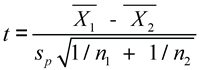
![]() and
and ![]() are the averages for the two groups.
are the averages for the two groups.
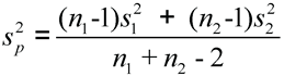
n1 and n2 are sample sizes for the two groups, and s1 and s2 are the standard deviations for the two groups.
For the unequal variances (unpooled) test, SAS uses the following calculation:

n1, n2, s1, and s2 are defined above.
Changing the Alpha Level for Confidence Intervals
SAS automatically creates 95% confidence intervals. You can change the alpha level for the confidence intervals with the ALPHA= option in the PROC TTEST statement. The statements below create 90% confidence intervals and produce Figure 8.8.[6]
ods select conflimits;
proc ttest data=bodyfat alpha=0.10;
class gender;
var fatpct;
run;

Compare Figures 8.7 and 8.8. The column headings in each figure identify the confidence levels. Figure 8.7 contains 95% confidence limits, and Figure 8.8 contains 90% confidence limits. All the other statistics are the same.
The general form of the statements to specify the alpha level using PROC TTEST is shown below:
PROC TTEST DATA=data-set-name ALPHA=level;
CLASS class-variable;
VAR measurement-variables;
level gives the confidence level. The value of level must be between 0 and 1. A level value of 0.05 gives the automatic 95% confidence intervals. Items in italic were defined earlier in the chapter.
Performing the Wilcoxon Rank Sum Test
The Wilcoxon Rank Sum test is a nonparametric test for comparing two independent groups. It is a nonparametric analogue to the two-sample t-test, and is sometimes referred to as the Mann-Whitney U test. The null hypothesis is that the two means for the independent groups are the same. The only assumption for this test is that the observations are independent.
To illustrate the Wilcoxon Rank Sum test, consider an experiment to analyze the content of the gastric juices of two groups of patients.[7] The patients are divided into two groups: patients with peptic ulcers, and normal or control patients without peptic ulcers. The goal of the analysis is to determine whether the mean lysozyme levels for the two groups are significantly different at the 5% significance level. (Lysozyme is an enzyme that can destroy the cell walls of some types of bacteria.) Table 8.5 shows the data.

This data is available in the gastric data set in the sample data for the book. Although not shown here, you could use PROC UNIVARIATE to investigate the normality of each group. The data is clearly not normal. As a result, the parametric two-sample t-test should not be used to compare the two groups.
The first four steps of analysis are complete.
1. Create a SAS data set.
2. Check the data set for errors. PROC UNIVARIATE was used to check for errors. Although outlier points appear in the box plots, the authors of the original data did not find any underlying reasons for these outlier points. Assume that the data is free of errors.
3. Choose the significance level for the test. Choose a 5% significance level, which requires a p-value less than 0.05 to conclude that the groups are significantly different.
4. Check the assumptions for the test. The only assumption for this test is that the observations are independent. This seems reasonable, because each observation is a different person. The lysozyme level in one person is not dependent on the lysozyme level in another person. (This fact ignores the possibility that two people could be causing stress—or ulcers—in each other!)
5. Perform the test. See “Using PROC NPAR1WAY for the Wilcoxon Rank Sum Test.”
6. Make conclusions from the test results. See “Finding the p-value.”
Using PROC NPAR1WAY for the Wilcoxon Rank Sum Test
SAS performs nonparametric tests to compare two independent groups with the NPAR1WAY procedure. To create the data set and perform the Wilcoxon Rank Sum test, submit the following code:
data gastric;
input group $ lysolevl @@;
datalines;
U 0.2 U 10.4 U 0.3 U 10.9 U 0.4 U 11.3 U 1.1 U 12.4 U 2.0
U 16.2 U 2.1 U 17.6 U 3.3 U 18.9 U 3.8 U 20.7 U 4.5
U 24.0 U 4.8 U 25.4 U 4.9 U 40.0 U 5.0 U 42.2 U 5.3
U 50.0 U 7.5 U 60.0 U 9.8
N 0.2 N 5.4 N 0.3 N 5.7 N 0.4 N 5.8 N 0.7 N 7.5 N 1.2 N 8.7
N 1.5 N 8.8 N 1.5 N 9.1 N 1.9 N 10.3 N 2.0 N 15.6 N 2.4
N 16.1 N 2.5 N 16.5 N 2.8 N 16.7 N 3.6 N 20.0
N 4.8 N 20.7 N 4.8 N 33.0
;
run;
proc npar1way data=gastric wilcoxon;
class group;
var lysolevl;
title 'Comparison of Ulcer and Control Patients';
run;
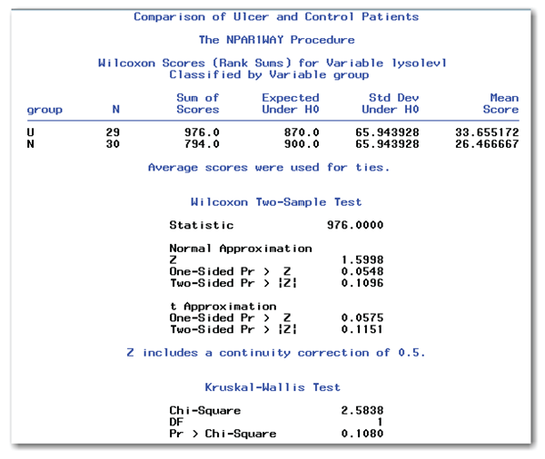
The WILCOXON option requests the Wilcoxon Rank Sum test. The CLASS statement identifies the variable that classifies the data into two groups. The VAR statement identifies the variable to use to compare the two groups. Figure 8.9 shows the results.
Figure 8.9 shows the Scores, Wilcoxon Two-Sample Test, and Kruskal-Wallis Test tables. Chapter 9 discusses the Kruskal-Wallis Test table, which is appropriate for more than two groups. The next two topics discuss the other two tables.
Finding the p-value
Figure 8.9 shows the results of the Wilcoxon Rank Sum test. First, answer the research question, “Are the mean lysozyme levels significantly different for patients without ulcers and patients with ulcers?”
In Figure 8.9, look in the Wilcoxon Two-Sample Test table and find the first row with the heading Two-Sided Pr > |Z|. Look at the number to the right, which gives the p-value for the Wilcoxon Rank Sum test. For the gastric data, this value is 0.1096, which is greater than the significance level of 0.05. You conclude that the mean lysozyme levels for the patients without ulcers and for the patients with ulcers are not significantly different at the 5% significance level.
In general, to interpret results, look at the number to the right of the first row labeled as Two-Sided Pr > |Z|. If the p-value is less than the significance level, you conclude that the means for the two groups are significantly different. If the p-value is greater than the significance level, you conclude that the means are not significantly different. Do not conclude that the means for the two groups are the same. (See the discussion earlier in this chapter.)
Understanding Tables in the Output
The list below describes the other items in the Wilcoxon Two-Sample Test table in Figure 8.9.
Statistic
is the Wilcoxon statistic, which is the sum of scores for the group with the smaller sample size.
Normal Approximation Z
is the normal approximation for the standardized test statistic.
Normal Approximation One-Sided Pr > Z
is the one-sided p-value, which displays when Z is greater than 0. When Z is less than 0, SAS displays One-Sided Pr < Z instead.
Normal Approximation Two-Sided Pr > |Z|
is the two-sided p-value, which was described earlier.
t Approximation One-Sided Pr > Z
Approximate p-values for the two-sample t-test. If the t-test is appropriate for your data, use the exact results from PROC TTEST instead.
t Approximation Two-Sided Pr > |Z|
Approximate p-values for the two-sample t-test. If the t-test is appropriate for your data, use the exact results from PROC TTEST instead.
Z includes a continuity correction of 0.5
Explains that PROC NPAR1WAY has automatically applied a continuity correction to the test statistic. Although you can suppress this continuity correction with the CORRECT=NO option in the PROC NPAR1WAY statement, most statisticians accept the automatic application of the continuity correction.
This list below describes the Scores table in Figure 8.9. The title for this table identifies the measurement variable and the classification variable.
Variable
identifies the name of the classification variable and the levels of this variable. The title and content of this column depend on the variable listed in the CLASS statement. In this example, the group variable defines the groups and has the levels U (ulcer) and N (normal).
N
is the number of observations in each group.
Sum of Scores
is the sum of the Wilcoxon scores for each group. To get the scores, SAS ranks the variable from lowest to highest, assigning the lowest value 1, and the highest value n, where n is the sample size. SAS sums the scores for each group to get the sum of scores.
Expected Under H0
lists the Wilcoxon scores expected under the null hypothesis of no difference between the groups. If the sample sizes for the two groups are the same, this value for both groups will also be the same.
Std Dev Under H0
gives the standard deviation of the sum of scores under the null hypothesis.
Mean Score
is the average score for each group, calculated as (Sum of Scores)/N.
Average scores were used for ties
describes how ties were handled by the procedure. Ties occur when you arrange the data from highest to lowest, and two values are the same. Suppose the observations that would be ranked 7 and 8 have the same value for the measurement variable. Then, these observations are both assigned a rank of 7.5 (=15/2). This message is for information only. There isn’t an option to control how ties are handled.
As discussed in Chapter 4, you can use the ODS statement to choose the output tables to display. Table 8.6 identifies the output tables for PROC NPAR1WAY and the Wilcoxon Rank Sum test.
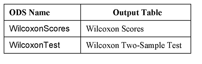
For example, the statements below create output that contains only the Wilcoxon Two-Sample Test table:
ods select wilcoxontest;
proc npar1way data=gastric wilcoxon;
class group;
var lysolevl;
run;
The general form of the statements to perform tests for equal variances and tests to compare two means using PROC NPAR1WAY is shown below:
PROC NPAR1WAY DATA=data-set-name;
CLASS class-variable;
VAR measurement-variables;
Other items were defined earlier.
The CLASS statement is required. The class-variable can have only two levels. While the VAR statement is not required, you should use it. If you omit the VAR statement, then PROC NPAR1WAY performs analyses for every numeric variable in the data set.
You can use the BY statement to perform several t-tests corresponding to the levels of another variable. However, another statistical analysis might be more appropriate. Consult a statistical text or a statistician before you do this analysis.
- Independent groups of data contain measurements for two unrelated samples of items.
- To summarize data for independent groups, summarize each group separately.
- To choose a statistical test, first, decide whether the data is from independent or paired groups. Then, decide whether to use a parametric or a nonparametric test. The second decision is based on whether the assumptions for the parametric test seem reasonable. Tests for the four cases are:

- Regardless of the statistical test you choose, the steps of analysis are:
1. Create a SAS data set.
2. Check the data set for errors.
3. Choose the significance level for the test.
4. Check the assumptions for the test.
5. Perform the test.
6. Make conclusions from the test results.
- Regardless of the statistical test, to make conclusions, compare the p-value for the test with the significance level.
- If the p-value is less than the significance level, then you reject the null hypothesis, and you conclude that the means for the groups are significantly different.
- If the p-value is greater than the significance level, then you fail to reject the null hypothesis. You conclude that the means for the groups are not significantly different. (Remember, do not conclude that the means for the two groups are the same!)
- Test for normality using PROC UNIVARIATE as described in Chapter 5. For independent groups, test each group separately.
- Test for equal variances using PROC TTEST when comparing two independent groups.
- When comparing two independent groups, what type of SAS analysis to perform depends on the outcome of the unequal variances test. In either case, use PROC TTEST and choose either the Equal or Unequal test.
- You can change the confidence levels in PROC TTEST with the ALPHA= option.
- Use PROC NPAR1WAY to perform the Wilcoxon Rank Sum test when the assumptions for the t-test are not met.
To summarize data from two independent groups
- To create a concise summary of two independent groups:
PROC MEANS DATA=data-set-name;
CLASS class-variable;
VAR measurement-variables;
data-set-name
is the name of a SAS data set.
class-variable
is the variable that classifies the data into groups.
measurement-variables
are the variables you want to summarize.
The CLASS statement is required. You should use the VAR statement. You can use any of the options described in Chapter 4.
- To create a detailed summary of two independent groups with comparative histograms:
PROC UNIVARIATE DATA=data-set-name NOPRINT;
CLASS class-variable;
VAR measurement-variables;
HISTOGRAM measurement-variables;
Items in italic were defined earlier. The CLASS statement is required. You should use the VAR statement. You can use any of the options described in Chapters 4 and 5. You might want to use the NOPRINT option to suppress output and view only the comparative histograms.
- To create comparative vertical bar charts as an alternative to high-resolution histograms:
PROC CHART DATA=data-set-name;
VBAR measurement-variables / GROUP=class-variable;
Items in italic were defined earlier. For comparative horizontal bar charts, replace VBAR with HBAR. The GROUP= option appears after the slash. You can use any of the options described in Chapter 4.
- To create side-by-side box plots, you might need to first use PROC SORT to sort the data by the class variable.
PROC SORT DATA=data-set-name;
BY class-variable;
PROC BOXPLOT DATA=data-set-name;
PLOT measurement-variable*class-variable;
Items in italic were defined earlier. The asterisk in the PLOT statement is required.
To check the assumptions (step 4)
- To check the assumption of independent observations, you need to think about your data and whether this assumption seems reasonable. This is not a step where using SAS will answer this question.
- To check the assumption of normality, use PROC UNIVARIATE. For independent groups, check each group separately.
- To test for equal variances for the two-sample t-test, use PROC TTEST and look at the p-value for the Folded F test. See the general form in the next step.
To perform the test (step 5)
- To perform the two-sample t-test to compare two independent groups, use PROC TTEST. Look at the appropriate p-value, depending on the results of testing the assumption for equal variances.
PROC TTEST DATA=data-set-name;
CLASS class-variable;
VAR measurement-variables;
Items in italic were defined earlier. The CLASS statement is required. You should use the VAR statement.
- To perform the nonparametric Wilcoxon Rank Sum test to compare two independent groups, use PROC NPAR1WAY. Look at the two-sided p-value for the normal approximation.
PROC NPAR1WAY DATA=data-set-name;
CLASS class-variable;
VAR measurement-variables;
Items in italic were defined earlier. The CLASS statement is required. You should use the VAR statement.
Enhancements
- To change the alpha level for confidence intervals for independent groups, use the ALPHA= option in the PROC TTEST statement.
The program below produces the output shown in this chapter:
proc format;
value $gentext 'm' = 'Male'
'f' = 'Female';
run;
data bodyfat;
input gender $ fatpct @@;
format gender $gentext.;
label fatpct='Body Fat Percentage';
datalines;
m 13.3 f 22 m 19 f 26 m 20 f 16 m 8 f 12 m 18 f 21.7
m 22 f 23.2 m 20 f 21 m 31 f 28 m 21 f 30 m 12 f 23
m 16 m 12 m 24
;
run;
proc means data=bodyfat;
class gender;
var fatpct;
title 'Brief Summary of Groups';
run;
ods select moments basicmeasures extremeobs plots;
proc univariate data=bodyfat plot;
class gender;
var fatpct;
title 'Detailed Summary of Groups';
run;
proc univariate data=bodyfat noprint;
class gender;
var fatpct;
histogram fatpct;
title 'Comparative Histograms of Groups';
run;
proc chart data=bodyfat;
vbar fatpct / group=gender;
title 'Charts for Fitness Program';
run;
proc sort data=bodyfat;
by gender;
run;
proc boxplot data=bodyfat;
plot fatpct*gender;
title 'Comparative Box Plots of Groups';
run;
proc ttest data=bodyfat;
class gender;
var fatpct;
title 'Comparing Groups in Fitness Program';
run;
ods select conflimits;
proc ttest data=bodyfat alpha=0.10;
class gender;
var fatpct;
run;
data gastric;
input group $ lysolevl @@;
datalines;
U 0.2 U 10.4 U 0.3 U 10.9 U 0.4 U 11.3 U 1.1 U 12.4 U 2.0
U 16.2 U 2.1 U 17.6 U 3.3 U 18.9 U 3.8 U 20.7 U 4.5
U 24.0 U 4.8 U 25.4 U 4.9 U 40.0 U 5.0 U 42.2 U 5.3
U 50.0 U 7.5 U 60.0 U 9.8
N 0.2 N 5.4 N 0.3 N 5.7 N 0.4 N 5.8 N 0.7 N 7.5 N 1.2 N 8.7
N 1.5 N 8.8 N 1.5 N 9.1 N 1.9 N 10.3 N 2.0 N 15.6 N 2.4
N 16.1 N 2.5 N 16.5 N 2.8 N 16.7 N 3.6 N 20.0
N 4.8 N 20.7 N 4.8 N 33.0
;
run;
proc npar1way data=gastric wilcoxon;
class group;
var lysolevl;
title 'Comparison of Ulcer and Control Patients';
run;
ENDNOTES
[1] Chapter 7 discusses comparing paired groups. For completeness, this table shows the tests for comparing both types of groups.
[2] If you are running a version of SAS earlier than 9.2, you will see headings of Upper CL Mean, Lower CL Mean, Upper CL Std Dev, and Lower CL Std Dev. The descriptive statistics appear in a different order. The output for earlier versions of SAS consists of the Statistics table and the T tests section.
[3] If you are running a version of SAS earlier than 9.2, you will see headings of Upper CL Mean and Lower CL Mean. The descriptive statistics appear in a different order.
[4] If you are running a version of SAS earlier than 9.2, you will see headings of Lower CL Std Dev and Upper CL Std Dev. The descriptive statistics appear in a different order.
[5] This output table is not available in versions of SAS earlier than 9.2. Instead, the confidence limits appear in the Statistics table.
[6] The Confidence Limits output table is not created for versions of SAS earlier than 9.2, so the ODS statement will not work for versions of SAS earlier than 9.2. Instead, use an ODS statement to request only the Statistics table, which contains confidence limits for versions of SAS earlier than 9.2. Also, see the footnote for Figure 8.7—the same differences in headings occur in Figure 8.8 for versions of SAS earlier than 9.2.
[7] Data is from K. Myer et al., “Lysozyme activity in ulcerative alimentary disease,” in American Journal of Medicine 5 (1948): 482-495. Used with permission.