

Chapter 5
SAS OLAP Cube Studio
Building Different Views of Your Data
5.1 Getting Started
5.1.1 Quick Tour
5.1.2 Prerequisites
5.2 Understanding OLAP Cubes
5.2.1 Understanding the Cube Structure
5.2.2 Understanding the Cube Terms
5.3 Creating OLAP Cubes
5.3.1 Preparing the Source Data
5.3.2 Designing a Cube Structure
5.3.3 Creating and Maintaining OLAP Cubes
5.4 Creating Your First OLAP Cube
5.4.1 Creating an OLAP Cube from Detailed Data
5.5 Creating a Cube from Star Schema Tables
5.5.1 Defining Star Schema Tables
5.5.2 Adding Dimensions with Star Schema Tables
5.6 Enhancing the Cube
5.6.1 Adding Time and GEO Dimensions
5.6.2 Working with Unbalanced or Ragged Hierarchies
5.6.3 Defining Calculated Members for Custom Measurements
5.7 Maintaining an OLAP Cube
5.7.1 Variations in Data Storage Techniques
5.7.2 Adding Custom Aggregations with the Aggregation Tuning Module
5.7.3 Scheduling the OLAP Cube Refresh
5.7.4 Updating In-Place
5.8 SAS Administrator Tasks
5.8.1 Granting Access to the OLAP Schema
5.8.2 Member-Level Security
Chapter 5
SAS OLAP Cube Studio
Building Different Views of Your Data
SAS OLAP Cube Studio allows you to easily and quickly transform your data into an online analytical processing (OLAP) structure. Data stored in an OLAP structure, which is called a cube, can be accessed from multiple SAS BI clients, including SAS Enterprise Guide, SAS Web Report Studio, and SAS BI Dashboard, to complete analysis, build reports, and even build other data structures.
An OLAP cube works particularly well with large data sets by reducing the time needed to access and display data. Performance is enhanced because data is summarized into measures and predefined into categories. Users are able to review the data from multiple angles so they can quickly answer questions without waiting for data summarizations or running various reports on the same source. The data can also be secured at levels within the cube, so one source can service many different users in the organization.
SAS OLAP Cube Studio guides you through the cube-building and maintenance process. This chapter explains how to use SAS OLAP Cube Studio to build a simple cube and introduces the features of the tool.
5.1 Getting Started
This topic provides an overview of the tool capabilities and what you need to get started.
5.1.1 Quick Tour
When you open SAS OLAP Cube Studio, the main window appears. From this window you can build, modify, and manage OLAP cubes. The two main areas you can use to navigate the metadata are the Folder and Inventory tabs. The following figure shows the default configuration for the application. Your system can display different information depending on the security structures and prior steps taken to organize metadata.

Figure 5.1-1. SAS OLAP Cube Studio main window
1 |
The Folders tab provides a navigation tree for the metadata. |
2 |
The Inventory tab provides a navigation tree for the metadata objects. The Cube folder shows all cubes that you can access. You can see the Candy_Sales cube (this is the same cube as shown in Projects folder) and some other cubes that are not stored in the same location as the Candy_Sales cube. This tab provides a quick way to access all objects. |
5.1.2 Prerequisites
Prior to using the application at your site, you must have the following:
- SAS OLAP Cube Studio application installed on your desktop
- Connection profile to the SAS Metadata Server
- Permissions to an OLAP schema
- SAS folder in the SAS Metadata Server to access and store the OLAP cube
Contact your SAS site administrator for more information or additional assistance.
Note: All examples within this chapter use the SAS OLAP Cube Studio; however, SAS Data Integration Studio provides the same graphical interface.
5.2 Understanding OLAP Cubes
OLAP cubes dramatically improve the ability to query large data structures. For small data structures, filtering on one or more categories and summarizing columns might take a few seconds, but for large tables that contain millions of records doing the same action could take several minutes. The other advantage to using cubes is that you can explore measures from a variety of viewpoints quickly.
The following topic explains how cubes are different from relational data structures and the terms used to describe a cube.
5.2.1 Understanding the Cube Structure
By now, you might be wondering how OLAP cubes are different from other data structures. If you have been working with reports and data, you are probably more familiar with relational or transactional data structures, where the data appears like a spreadsheet. The spreadsheet columns can be categorized, filtered, and counted. This is called transactional data because each row of the data represents a single transaction.
In the following figure, each row has the sales amounts
summarized by category for the sales amount. You can also see how the data is
organized; for example, ![]() State is a
category for Country and
State is a
category for Country and ![]() PRODTYPE is
segmented by Product. From the
PRODTYPE is
segmented by Product. From the ![]() Date column, you could easily extract data for the year, quarter, or month.
Date column, you could easily extract data for the year, quarter, or month.

Figure 5.2-1 Example of Relational Data Source
If you want to create a report for this data, there are several ways to organize the information, such as summarizing the sales as year-to-date amounts by product, geography, or some combination of all. However, it would take several different reports to display this data for analysis. If this data is actually a million-record data table, the report could take a while to display.
Many times users are not trying to determine how many sofas were sold on a certain day; rather, they want the data summarized by country, state, product, and date so they can slice and dice the data to find patterns and trends. An OLAP cube makes this possible by providing all of the likely paths through pre-calculated measures across the data.
Relationships between data, such as Country and State; Product Type and Product; or Year, Quarter, and Month can be logically grouped into dimensions. Each grouping contains defined hierarchies that establish a path for users to drill into for more details. For example, a time dimension containing data for Year, Quarter, Month, and Day might contain two hierarchies. One hierarchy takes users from Year to Month to Day and the second hierarchy allows them to drill from Year to Quarter to Month. Each of the individual data columns used to compose the hierarchy is termed a level.
The following figure represents a cube structure with each side corresponding to a dimension and hierarchy. The measure within the cube is Actual Sales. Turning the cube or drilling into the hierarchy the measure Actual Sales will have a different sum based on your current view.

Figure 5.2-2 Cube with multiple dimensions
In the following figure, you can see how a cube looks in the SAS Enterprise Guide OLAP Viewer. You can see the Region and Product dimensions for the sales amount as sum and average. In Section 5.4, “Creating Your First OLAP Cube,” you will learn how to create this cube.

Figure 5.2-3 Example of a cube in the OLAP Viewer
5.2.2 Understanding the Cube Terms
There are five cube terms to learn: dimensions, hierarchies, levels, members, and measures. In the following figure, a cross-tabular report is shown using cube data.

Figure 5.2-4 Cube structure layout example
This table defines each cube term listed in the previous figure and provides an example data item or structure.
| Term | Definition | Examples | |
|---|---|---|---|
1 |
Dimensions |
Provides a grouping of natural elements that helps answer the key questions who, what, where, when, and how. In the example, the dimensions are country and product. |
|
2 |
Hierarchies |
Identifies the path to move along for more details and summarizes the dimensions. This can be thought of as a parent-child relationship. For example, in the figure, Country is the parent to State/Province. At a minimum, one hierarchy is defined within each dimension. Note: The total number of hierarchies used across all dimensions cannot exceed 128. |
|
3 |
Levels |
An individual column that is used to make up a hierarchy. Levels in the above example include Country, State/Province, and Product. Note: Within a hierarchy, up to 19 levels can be used. The total number of levels that can be used within a cube is 256. |
|
4 |
Measures |
Identifies the statistics available for each dimension. In the example, Sum of Actual Sales and Average of Actual Sales are measures. You can also create custom measures based on other measures. For example, percentages or ratios. Note: A maximum of 1024 measures per cube is possible. |
|
5 |
Members |
Represents an individual data element. You can use members in PROC OLAP code to create advanced measurements. Note: The maximum number of members is 232 per hierarchy. |
|
5.3 Creating OLAP Cubes
There are three steps to follow when creating OLAP cubes:
- Preparing the source data
- Designing the structure (dimensions, hierarchy layout, and measures)
- Creating and maintaining the cube
5.3.1 Preparing the Source Data
Before you can build a cube, you must have a data source. A data source can be a single SAS data set or a group of star schema data sets, which are joined when the cube is created. Your choice for the data source depends on several factors, such as available tables, amount of data, and user requirements.
SAS OLAP Cube Studio allows you to use one of three different data sources: detail table, fully summarized table, or star schema tables.
5.3.1.1 Detail Tables
This data source closely resembles the spreadsheet structure: it contains information for every measure and member necessary to generate the cube structure. In the following example, you can see an example extract of a detail table. This data represents individual transactions for each product for a particular month. SAS OLAP Cube Studio summarizes these records into the defined dimensions.
| Country | State | Type | Product | Date | Actual Sales |
|---|---|---|---|---|---|
Canada |
Quebec |
Office |
Chair |
01FEB11 |
10,000 |
Canada |
Quebec |
Office |
Chair |
15FEB11 |
12,000 |
Mexico |
BAJA |
Office |
Chair |
01FEB11 |
20,000 |
Mexico |
BAJA |
Office |
Chair |
15FEB11 |
12,500 |
USA |
CA |
Office |
Chair |
01FEB11 |
74,000 |
USA |
CA |
Office |
Chair |
15FEB11 |
75,500 |
Table 5.3-1 Example of detail table data source
5.3.1.2 Fully Summarized Table
This data source is already summarized to the lowest level for all dimensions. The following figure shows an extract of the data in Table 5.3-1 after it has been summarized. The actual sales have been totaled by each dimension, resulting in the February sales.
| Country | State | Type | Product | Month | Actual Sales |
|---|---|---|---|---|---|
Canada |
Quebec |
Office |
Chair |
FEB11 |
22,000 |
Mexico |
BAJA |
Office |
Chair |
FEB11 |
32,500 |
USA |
CA |
Office |
Chair |
FEB11 |
149,500 |
Table 5.3-2 Example of a fully summarized data source
When the data is summarized to its lowest level of all analyzed variables, it is called an n-way summary. You can use a SAS procedure called PROC SUMMARY to create summarized data before using SAS OLAP Cube Studio. Following is an example of PROC SUMMARY that creates the fully summarized table.
/*=============================================================*/ /*Create an NWAY summary for all levels in the data set */ proc summary data=SASHELP.PRDSAL3 nway; class country state prodtype product date; var actual_sales; output out=mylib.class_sum sum(actual_sales)=actual_sales; run; /*========================================================================*/ |
Program 5.3-1 Sample summary procedure code for PRDSAL3
5.3.1.3 Star Schema Tables
Star schema data sources consist of multiple dimension tables and one additional table known as the fact table. Fact tables are joined to the dimension tables by key variables. In the following figure, a fact table is in the center with four dimension tables surrounding it, resembling a star. The fact table contains the numeric or aggregate values for each dimension, and the dimension tables contain the data categories. For example, in this figure, the fact table has several key variables, such as Prod_ID, Region_ID, and so on. For each key variable, there is a dimension table with a matching key.

Figure 5.3-1 Star schema data source
In the following figure, you can see an example of how the
raw data in each table appears. The fact table ![]() lists the ProdID key variable with the value of 7. This correlates to the
ProdID in the Product dimension table
lists the ProdID key variable with the value of 7. This correlates to the
ProdID in the Product dimension table ![]() .
The Product dimension table has a hierarchy of Category > Subcategory > Product.
SAS OLAP Cube Studio automatically creates the join when you define the
dimension.
.
The Product dimension table has a hierarchy of Category > Subcategory > Product.
SAS OLAP Cube Studio automatically creates the join when you define the
dimension.

Figure 5.3-2 Linking from a Fact table to a Dimension table
For larger tables with many dimensions, it is easier to manage the data when it is organized in this structure. The benefit of using a star schema is to speed data retrieval and have the data formatted in a way that is easy to understand and maintain.
The snowflake schema is a variation of the star schema where two or more dimension tables are joined together before joining with the fact table. An example of the snowflake schema is a product dimension table that contains IDs that link to product type and group dimension tables, while the fact table contains an ID linking only to product dimension. Snowflake schemas are not directly supported by SAS OLAP; conversion of the dimension table joins into a single table (or view) is required before beginning the OLAP definition.
 In order for SAS
OLAP to retrieve snowflake schema’s additional dimension tables, the tables
must first be converted into a single dimension table or view.
In order for SAS
OLAP to retrieve snowflake schema’s additional dimension tables, the tables
must first be converted into a single dimension table or view.
5.3.2 Designing a Cube Structure
Designing a cube is somewhat of an art. After building an initial cube, you might have to redesign it several times before it is ready for production. Preparing the data, understanding the requirements, and planning the dimensions and measures will increase your success.
5.3.2.1 Organizing Your Data
After learning the OLAP terms, you might already have some ideas about the cube structure. The logical dimensions and hierarchies, such as time (year, month, day) or geographical (country, state, city) and logical measures, such as sum of sales and count of units, will quickly fall into place.
When creating the cube, it is helpful to begin with the end in mind. The first thing to consider is how end users will interact with the cube when it is used in a report and what they are trying to measure. For instance, department managers are interested in how close, in dollars, they are to exceeding their budget. For the cube to be useful for the end user, the data must be logical and easy to navigate. Users might quickly abandon the cube if the path or level they need is missing.
Before starting SAS OLAP Cube Studio, you must prepare your data. Consider the following questions when designing the cube:
- Dimensions
- What paths will end users explore?
- What questions are the users asking about the data?
- What natural hierarchies and levels exist in my data, such as Time and Location?
- What hierarchies do I need to create?
- Product lines might need data from several tables moved to one
- Departments structures might not exist in a central area or be maintained
- Measures
- How does the data need to be calculated?
- Widgets sold
- Mean time to failure
- Average customer calls per month
- Do I have the needed data to generate the calculations?
- How does the data need to be calculated?
5.3.3 Creating and Maintaining OLAP Cubes
OLAP cubes can be created in one of two ways: writing the code in SAS Enterprise Guide using the OLAP procedure or using SAS OLAP Cube Studio.
In some sense, the cube design process never ends. As the end users employ the data for analysis and reporting, they will discover additional needed dimensions and measures. Cube maintenance includes tasks such as scheduling cube refreshing, reducing storage space, or improving performance of queries for end users. In Section 5.7, ”Maintaining an OLAP Cube,” you will learn more about cube maintenance.
SAS also
supports access to its OLAP technology using multidimensional expressions
(MDX), which allows for custom queries and measurements using functions similar
to those found in other vendor applications, such as Microsoft Analysis Cubes,
Oracle, and SAP.
5.4 Creating Your First OLAP Cube
This topic demonstrates how to use the SAS OLAP Cube Studio wizard to create a cube for a fictitious furniture company. The data is detailed in one table and the end result is shown in Figure. This simple cube has two dimensions and several measures.
Note: The OLAP cube created in this example is used to create a report in Chapter 7, “SAS Web Report Studio.”
5.4.1 Creating an OLAP Cube from Detailed Data
Use the following steps to create a cube:
- Open SAS OLAP Cube Studio and select New>Cube to start the Cube Designer wizard.
- Complete the fields in the initial page Cube Designer – General and select the Next button to continue.
Note: The numbers in the table correspond to the following figure.
Field Name Description 1
Name
The cube name can be up to 32 characters long.
Do not
include spaces within the name field. Certain functions do not act as
expected when spaces are embedded within the name.2
Description
Enter a description of what the cube contains. This information can be useful for users accessing the cube from other locations.
3
OLAP schema
Displays the list of available OLAP schemas defined within the metadata server. The OLAP schema defines to the metadata server which SAS OLAP Server runs the cube. The default OLAP schema is SASApp—OLAP Schema.
4
Location
Choose a metadata folder location where appropriate security is applied. This is where the users can find the cube.
5
Physical cube path
Select a physical path on the server to store the cube.
6
Input Type
Select the input type that matches your data source. There are three choices: Detail Table, Star Schema, and Fully Summarized Table. Refer to Section 5.3.1, ”Preparing the Source Data,” for a more complete description.
7
Include secured member values in presummarized computations
Optional If member-level security is applied and you want to enforce it throughout views, ensure that this check box is blank.
Refer to section 5.8.2, ”Member-Level Security,” for more detail.
- Select your data sources in this step by defining the input and drill-through data tables. Depending on the input type selected in the first
step, these windows can be slightly different.
Note: If you are creating a cube from with a star schema data source, refer to Section 5.5, “Creating a Cube from Star Schema Tables,” for more information.The first window requests the Input table, which contains all levels and measures required to build the OLAP cube. The second window requests the Detail table, which is used when users are allowed to drill through to detail on a report. If the data source does not appear in the available tables, it might not be registered with the metadata server. If you have Write Metadata Access to a particular folder, you can define new tables on this window by selecting the Register Table button.
Click the View Data button to
see a preview of the source data to ensure that you are selecting the correct
table.- In
the Cube Designer – Input page, select the input data source. Move the data
source to the right side. In the following figure, PRDSAL3CUBE was selected and
displays in the Selected
table area. Click the Next button to continue.

- In the Cube Designer – Drill-Through page, select the data source that is used for the drill-through. Typically, when using the Detail Input type, the input and drill-through uses the same data source. Click Next to continue.
In fully
summarized tables, you can use the same table or the source table that was used
when creating the fully summarized table. When using a different table as the
detail source, you must ensure that each variable in the cube design is
represented in the table.
- In
the Cube Designer – Input page, select the input data source. Move the data
source to the right side. In the following figure, PRDSAL3CUBE was selected and
displays in the Selected
table area. Click the Next button to continue.
- In the Cube Designer – Dimensions page, you can setup the dimensions. Click the Add button to create a dimension.
For this example, this is a simple dimension called Region comprised of Country and State. The raw data is shown in Figure 5.2-1, Example of Relational Data Source.
- Complete the fields in the Dimension Designer-General window and click Next to continue.

Field Name Description 1
Name
The name of the dimension cannot be the same as the name of any levels.
If you have a variable called Region in the data table and you name the dimension Region, an error message is generated. In the example, the dimension is called Region.
2
Caption Description
Use the Description field to explain what levels are included in the dimension. This field is optional.
The user sees this value when viewing the cube directly from BI clients such as SAS Add-In for Microsoft Office and SAS Enterprise Guide. It is a good practice to make the description as descriptive as possible.
3
Type
You can select three types: Standard, Time, and GEO.
Most of the time the type is Standard. Refer to Section 5.6.1, “Adding Time and GEO Dimensions,” for more information about how to use the other types.
4
Sort order
Affects how the data is displayed when directly accessed from tools such as SAS Add-In for Microsoft Office and SAS Enterprise Guide.
Sort order is
not maintained when a cube is accessed through an information map.5
Star Schema Table
When dimension data is contained within the fact table itself you should select this option. This is used only when working with data arranged as a star schema.
Refer to Section 5.5, “Creating a Cube from Star Schema Tables,” for information on adding dimensions for star schema data.
- In the Dimension Designer – Level page, you can select the levels that belong to the dimension. The first dimension, called Regional Stores, has two levels, Country and State. To define the Levels, click the Add button.
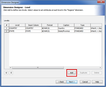
- In the Add Levels window, select the variables you want to add. Click Next to continue.
If there will
be only one hierarchy, you can choose the levels in the order they are used in
the hierarchy. This step saves time during hierarchy definition.

- To set the hierarchy order for the dimension, you must add a hierarchy. Click the Add button to create a hierarchy.
Select the Finish button for
SAS to automatically create the hierarchy and skip the next step. For this step
to work correctly, select the data fields for your dimension in the desired hierarchal order.

- In the Available
input columns area, drag the fields to the selected area in the
correct order. Select OK to continue. Then click the Finish button to continue creating the cube.

- Complete the fields in the Dimension Designer-General window and click Next to continue.
- In this step, you select the measures used in the cube. You must select
at least one available measure to move forward. These measures are calculated
during the cube building process; therefore, certain calculations (such as a
ratio) are not available at this point.
Calculated
members such as a ratio are defined and stored within the metadata and
calculated at run time, no matter the cube type.

In the lower half of this window, you have the ability to define measures based on unique member counts. An example is when you need the Number of Customers as a measure on your report, but your data table contains the customer name.
- In the Cube Designer - Measure Details page, you can set the default measure and adjust the labels and formats for measures.

Field Name Description 1
Default measure
Define the default measure users see when initially opening the cube directly in SAS Add-In for Microsoft Office or SAS Enterprise Guide. Select the one that seems more appropriate. In this case, sum of sales is chosen.
2
Measure Name
This name is used in backend queries; these names must not have spaces.
3
Input Column
The source table column used to derive the measure.
4
Statistic
The statistic function used to summarize the data.
5
Caption
Name of the measure that is displayed for users. You can modify this name so it is more user-friendly if necessary.
6
Format
Format of the measure that is displayed to users. You can modify this format to match the statistic. For instance, the DOLLAR12 option causes the dollar sign ($) to display in front of the value.
- In simple OLAP structures, no member properties are required for an OLAP cube. This step is optional and you do not need to change the default settings selections in this window. Select Next to continue.
Member properties are attributes of dimension members that provide additional information to cube users. Member property information is usually not as significant as the levels and members within a dimension, and therefore does not qualify as a level or member. However, it can have additional analytical value that can be useful at query time.
- You can add aggregations to the cube during the creation process. This step is optional and you do not need to change the default settings selections at this window. Click Next to continue.
For more information about adding aggregations or using aggregations to improve cube performance, refer to Section 5.7.2, “Adding Custom Aggregations with the Aggregation Tuning Module.”
- When the wizard is complete, you can review the cube information. To
build the cube, select the first radio button. If you have created this cube
before, this button deletes and re-creates any existing cubes.
To save the
code for use in SAS Enterprise Guide, select the Export Code button.

5.5 Creating a Cube from Star Schema Tables
When creating a cube with star schema tables, there are two times in the cube creation process where the process varies from how the other cube types are created. The first is when selecting the data and the second occurs when creating the dimensions. For a description of star schema tables, refer to Section 5.3.1.3, “Star Schema Tables.”
5.5.1 Defining Star Schema Tables
When building a star schema cube, you need to specify the
input fact table, dimension tables, and a drill-through table. In the Cube
Designer - Input page, provide the fact table ![]() for the cube, shown in the following figure. The fact table contains the join information and measures. In the Dimension Tables page, add all the required dimension tables
for the cube, shown in the following figure. The fact table contains the join information and measures. In the Dimension Tables page, add all the required dimension tables ![]() to the Selected tables area.
to the Selected tables area.

Figure 5.1-1 Choosing data sets for star schema data sources
In the next step, you are prompted to provide the drill-through table. The drill-through table in this scenario requires a view either with all the joins defined or a full detail table.
With star schema structures, an SQL view must be developed and registered separately for drill-through to detail functionality to work. Users can create this join in SAS Enterprise Guide or SAS Data Integration Studio and update library metadata with the table structure.
5.5.2 Adding Dimensions with Star Schema Tables
When adding dimensions using star schema data sources, the Dimension Designer interface provides an area to define the relationship between the fact table and the dimension tables. In the dimension table, the hierarchy is Product > Category > Subcategory. The common variable ProdID joins the two tables when you build the dimension. Refer to Section 5.5, “Creating a Cube from Star Schema Tables,” for an example of how star schema tables are joined.
To create a dimension from a star schema table, do the following:
- At the Cube Designer – Dimensions page, select the Add button to start
a new dimension.

- In the Dimension Designer – General page, complete the Star Schema Table area, and then continue with the dimension creation.
 The check box to Use
the fact table should be selected on the Cube Designer- Input
table page when all the levels for the dimension reside in the fact table.
The check box to Use
the fact table should be selected on the Cube Designer- Input
table page when all the levels for the dimension reside in the fact table.Field Name
Description
1
Table
Select the dimension table with the key variable.
2
Key/Fact key
Values in these drop-down fields establish the relationship between the tables. In this example, ProdID is selected, but the variables do not have to have the same name.
Key – Corresponds to a column in the dimension table.
Fact key - Represents the fact table column.
3
Table options
You can set any data set options, such as a WHERE clause, for the selected dimension table.
5.6 Enhancing the Cube
SAS OLAP Cube Studio makes enhancing the cube easy. You can create time and location dimensions, address missing data, and create custom measurements.
5.6.1 Adding Time and GEO Dimensions
There are two special dimension types available when creating a cube: time and GEO. These dimension types have special properties that make creating the cube easier.
5.6.1.1 Adding Time Dimensions
When adding a time-specific dimension such as Year > Quarter > Month, you can take advantage of the built-in time hierarchies. After selecting Time as the dimension type, the Add supplied time hierarchies choice becomes available on the Dimension Designer – Level page, as shown in the following figure.
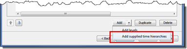
Figure 5.6-1 Add time dimensions
The Add Supplied window appears and you can choose a supplied time hierarchy structure. These supplied time hierarchies help build the dimension and auto-populate the levels and some level properties for the cube, reducing the time required to complete these windows.
The value in the Input column field must be
a date or date/time value for the hierarchy to work properly.
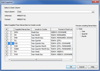
Figure 5.6-2 Using Add Supplied window
Time-series functions including rolling totals, rolling averages, and parallel period comparisons are enabled when a time dimension is defined, providing another benefit of using this dimension type.
5.6.1.2 Adding Geographic Locations with the ESRI Map Component
You can add geographic locations to your cube using the GEO dimension choice if you have an ArcGIS Server licensed at your organization. This is a separate product sold by Esri, not sold by SAS.
To use geographical locations, you must have the data set up properly. To avoid errors, data quality is extremely important, as there must be a match between the field ID in the map with the field ID in the cube input table. Within the Esri ArcMap, a layer should be defined for each level in the OLAP dimension. The ArcMap layer must contain the Map Service field ID information, along with the polygon details. An example of this mapping is shown in the following table.
OLAP Level |
Cube
Input Table |
Map Service Layer |
Map Service Field ID |
State |
StateFIP |
TL_2009_State |
StateFIPID |
County |
COFIP |
TL_2009_County |
CNTYIDFIP |
City |
PLCIDFP |
TL_2009_Place |
PLCIDFP |
Table 5.6-1 GEO mapping data
To create the geographic location, do the following:
Before adding a GEO dimension, create an Esri map using Esri ArcMap and create the Esri map service using the Esri ArcCatalog.
- At the Dimension Designer – General page, select GEO in the Type drop-down box. The GIS Maps button on the Dimension Designer is enabled and available for use.

- Select the GIS Maps button to open the GIS Maps Definition window. From here you must select a defined Esri Map Server and a running map service, and then connect the dimension levels to the map data.

5.6.2 Working with Unbalanced or Ragged Hierarchies
Customarily, there is one value in each level through a hierarchy, such as for dates: Year, Month, Day; or 2011, June, 10. In situations where there are gaps in the hierarchy, there are several options that can be applied to individual dimensions or the entire cube. An example is an organizational chart where there are gaps in the levels of the hierarchy for different members, which is called a ragged hierarchy.
Query
performance is impacted when missing members are not appropriately defined.

Figure 5.6-3 Ragged hierarchy example
If you consider the path to the Vice President ![]() under the Chief Information Officer, the member would look like the following:
under the Chief Information Officer, the member would look like the following:
[Organization].[All Organization].[Chief Executive Officer].[Chief Information Officer].[Vice President]
However, the member for the Administrative Assistant ![]() looks likes the following example:
looks likes the following example:
[Organization].[All Organization].[Chief Executive Officer].[ ].[ ].[ ].[Administrative Assistant]
Because this member does not have the same structure, the missing levels are represented with empty brackets. You can adjust the settings for an entire OLAP cube level or for individual dimensions. When the settings are in place, the same member would look like the following example. In this member, the empty brackets are not in the path.
[Organization].[All Organization].[Chief Executive Officer].[Administrative Assistant]
5.6.2.1 Adjusting the Settings for Missing Data
To adjust the settings for the missing data, use the following hints.
Change settings for Entire Cube: To adjust the ragged hierarchy settings for the entire cube, select the Advanced button from the Cube Designer – General page. From the Advanced Cube Options window, click the check boxes to ensure that the missing data is handled appropriately.
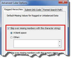
Figure 5.6-4 Change setting for entire cube
Change Settings for One Dimension: For a single dimension, select the Advanced button on the Dimension Designer – General page. In the Advanced Dimension Options window, you can choose to inherit the cube settings. You can also override the cube settings and make changes to the character and numeric values for the dimensions.

Figure 5.6-5 Change settings for one dimension
5.6.3 Defining Calculated Members for Custom Measurements
After creating the cube, you can add custom measurements. These measures are available for users from any interface and essentially appear the same as the measures you defined during the cube building process. The key difference is that these measures are not calculated and stored within the cube itself, but are only defined. When the user views the cube, the calculations are completed at run time and will change as the user manipulates the cube views.
There are three available starting points for a calculated member definition:
| Simple GUI |
|
| Time |
|
| Custom | Opens a definition window to define the measure name and
format. This allows you to use multidimensional expressions (MDX) code to
create a custom measure. Microsoft Corporation initially developed the MDXreference code as part of the OLE DB for OLAP specification.
|
5.6.3.1 Creating a Custom Measurement
After developing the cube, you can open the Calculated Members window by right-clicking the OLAP cube and then selecting Maintain > Calculated Members. In the following figure, Sum of Actual was created within the Furniture Sales cube. The remaining three columns are calculated members using the Time Series option.

Figure 5.6-6 Creating custom measurements
To create a calculated member, do the following:
- Right-click the cube you want to have the new calculated member. Select Maintain > Calculated Members.

- From the Calculations window, select the Add button to create a new calculation.
- Select Time Analysis Calculation from the Calculation Type window.
- In the Time Calculations page, select the Average Over Time radio button. For the Formula,
select the existing measure, a time period, and the number of periods for the
analysis. Select Next to continue.
In the following figure, the new member is the average sales for the last three periods.
- In the General page, type the name and select a format. Because the end user sees this name, try to be as descriptive as possible. You can also change the format. For this example, actual sales is a dollar value, so the format was changed to DOLLAR15. Click Next to save the measure.

5.7 Maintaining an OLAP Cube
If a cube was not created properly or regularly maintained, you might notice that it takes longer to generate, requires more system resources, and still does not deliver the promised speed and ease of use for the end users. In this section, you will learn some techniques for keeping your cubes in top shape.
5.7.1 Variations in Data Storage Techniques
There are several flavors of cubes. The most confusing part of OLAP for many users is the differences in MOLAP, ROLAP, and HOLAP.
MOLAP |
This is the default storage technique. This is where the summarization is calculated in advance and stored within the physical structure of the OLAP cube. This technique is best for performance because the aggregations are done ahead of time. All aggregations are stored on the server for quick retrieval. For large data sets, there might be sizing constraints for building the aggregations, making ROLAP a better choice. |
ROLAP |
The R represents relational, and gives users the ability to save the data outside of the OLAP cube in a flat or relational data set structure. This technique works well in these situations:
Performance for queries is dependent on the relational data tables. Users might find that this mechanism is much slower than MOLAP. |
HOLAP |
Hybrid OLAP offers some of both MOLAP and ROLAP storage techniques. Essentially, the structure is a ROLAP approach; however, the OLAP creator chooses to create several aggregations that are precalculated, so common queries and reports off this data generate results quickly. |
When editing the cube or creating a new one, the Cube Designer – Aggregations page provides an option to turn off NWAY aggregation. Selecting this check box changes the cube data storage from MOLAP to either HOLAP or ROLAP.

Figure 5.7-1 Setting the NWAY aggregation
5.7.2 Adding Custom Aggregations with the Aggregation Tuning Module
You can also create custom aggregations by selecting the Add button on the screen shown in Figure 5.7-1. However, with large or complex cubes, use the Aggregation Tuning dialog box from SAS OLAP Cube Studio. This mechanism analyzes log files or the data cardinality to assist with creating appropriate aggregations.
If users are complaining that OLAP-based reports are taking significant time to generate, consider adding custom aggregations to the cube. By default, OLAP cubes are stored with the NWAY aggregation only.
Use the Aggregation Tuning dialog box to analyze the OLAP logs and discover more dimensional cross joins to aggregate during the cube build process. Saved aggregations are stored within the OLAP definition and each time an OLAP cube is refreshed, these levels are recalculated and saved in the physical location with other aspects of the cube.
Within the dialog box there are three different mechanisms are available to add aggregations using this module: ARM Log, Cardinality, and Manual.
5.7.2.1 Creating the ARM Log
When using the ARM Log mechanism, the logging output must be increased to include the query detail. From SAS Management Console, complete the following steps to turn on logging:
- Select the Plug-ins tab.
- Expand Server Manager > SASApp > SASApp - Logical OLAP Server.
- Right-click on SASApp - OLAP Server and select Connect. The application connects to the server and the right panel shows the connections.

- Select the Loggers tab and locate the Perf.ARM.OLAP_SERVER logger. Select Properties to display the Perf.ARM.Olap_Server Properties window.

- Click the Assigned radio button and select Information from the drop-down list. This allows the server to capture the cube usage. Click OK to exit.

- Use the cube in a manner that simulates actual usage for best results. For instance, if the cube is mainly used with SAS Web Report Studio, then run a report using that application. The log needs to capture a representative sample of the common OLAP cube uses. It is a good idea to use the cube in the other applications for additional data.
- Once the log is completed and ready for use by the Aggregation Tuning function, you should repeat these steps to return the logging level to the Inherited>Error choice.
The log files can grow exponentially and performance can be impacted when the logs are allowed to run without boundaries.
5.7.2.2 Analyzing the ARM Log
When the ARM log is ready for review, do the following to analyze the log.
- In SAS OLAP Cube Studio, right-click the cube that you want to analyze and select Aggregation Tuning from the pop-up menu.
- From the Arm Log tab, select the Browse button to point to the ARM Log created in the OLAP process.
The typical location is within the configuration directory, such as:
<configuration directory>Lev1SASAppOLAPServerLogs - Select the radio button that creates the aggregation recommendations.
- Select the Analyze button to define possible aggregations for inclusion within the OLAP cube.
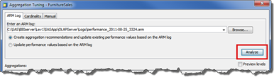
- After aggregations are developed, you have the option to remove the aggregation from inclusion in the next OLAP build (using the Delete or Drop buttons).
- Once completed, select the Update Aggregations button to create these aggregation tables for the OLAP cube to use.
The analysis on the Cardinality tab reviews the number of distinct members within each level of the cube; those with the highest cardinality are listed. Note that only 100 aggregations can be built at a time with this tool. However, after building a set of 100, you can add more.
In the following figure, you can see an example of recommendations based on the user interactions with the OLAP cube, as detailed in the ARM log created in the prior steps.

Figure 5.7-2 Example recommendations
5.7.3 Scheduling the OLAP Cube Refresh
Several mechanisms are available to schedule the OLAP cube refresh. From SAS Management Console, the OLAP job can be scheduled for routine refresh. Alternatively, you can export the short code and schedule the refresh using your native scheduler.
5.7.3.1 Using the Cube Job
Each time a cube is defined, a cube job is created automatically. The cube job provides metadata information, which can be used to deploy and schedule refreshes of the cube data or move a single cube from one system to another.
In the following figure, you can see where the jobs are
located in each tool. In SAS Management Console, the cube jobs are located
within the same metadata folder ![]() that the cube is stored in. In SAS OLAP Cube Studio, the Inventory tab has an expandable tab called Job (cube)
that the cube is stored in. In SAS OLAP Cube Studio, the Inventory tab has an expandable tab called Job (cube) ![]() .
.

Figure 5.7-3 Cube job location
Before scheduling a job in the Schedule Manager plug-in for SAS Management Console, the job must be deployed for scheduling in SAS OLAP Cube Studio.
- In SAS OLAP Cube Studio, right-click the job (cube) you want to change and select Scheduling > Deploy from the pop-up menu.
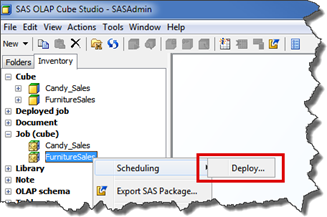
- Define the job on the batch server, as shown in the following figure.

The deployment directory is the location for a .SAS file that you then schedule using the Schedule Manager in SAS Management Console.
If you receive an error before this step, you must define a SAS DATA Step Batch Server within SAS Management Console. Refer to the SAS user documentation at support.sas.com for assistance. - From the Schedule Manager in SAS Management Console, select New Flow and schedule the deployed job for a routine refresh.

5.7.3.2 Using SAS Code
After creating the cube, you might want to make further changes to the code by using SAS Enterprise Guide, or provide the code to others. To export the code from SAS OLAP Cube Studio, select the cube and choose Export Code. In the Export Code window, select the Long form option and select the location to store the program.

Figure 5.7-4 Exporting the OLAP code
Open the newly
exported SAS program and uncomment the first PROC OLAP step by surrounding the
comment block top and bottom lines with /* */. Then a native scheduler can be
used to set up the routine refresh.
5.7.4 Updating In-Place
If a user session is active and has the cube locked, it can block the cube from refreshing the data. Some organizations have programmed mechanisms to automatically stop and restart the SAS OLAP Server to force a disconnection of users before refreshing cubes. This requires limited cube refresh times, such as overnight or on the weekend. For international companies, this proved extremely problematic as the window that all users are off the system can be extremely limited. In SAS OLAP Cube Studio, you can refresh the cube with new data in-place.

Figure 5.7-5 Select the Update In-Place menu choice
All existing connections to the cube remain intact while new connections use the new cube. Once all existing connections have been closed, the old cube is removed automatically. This action is done in-place, which means that it is invisible to the user community; the cube name, metadata location, and physical location remain the same.
The official switch between cubes can consume a significant amount of time if a large number of sessions access the cube; therefore, you can force an implementation of the refreshed data using the Disable and Enable menu elements.

Figure 5.7-6 Select Enable menu choice
These steps can be completed programmatically and
scheduled. The OLAP procedure has options ![]() (ADD_DATA, UPDATE_INPLACE, and UPDATE_DISPLAY_NAMES) that can be added to the code
to perform an in-place update.
(ADD_DATA, UPDATE_INPLACE, and UPDATE_DISPLAY_NAMES) that can be added to the code
to perform an in-place update.
/* ===================================================== */
PROC OLAP
 CUBE = "/Projects/Cubes/Candy_Sales"
 DATA = candy.CANDY_SALES_SUMMARY
![]()
ADD_DATA UPDATE_INPLACE UPDATE_DISPLAY_NAMES
;
/* ===================================================== */
Program 5.7-1 Update in place
To program the disable and enable steps, use the OLAPOPERATE
procedure options ![]() , as shown in the
following code:
, as shown in the
following code:
/* =============================================================*/
PROC OLAPOPERATE;
CONNECT USERID="sasadm@saspw" PW="xxxxxx" HOST="hostname" PORT=5451;
![]()
DISABLE CUBE "/Projects/Cubes/Candy_Sales";
 ENABLE CUBE "/Projects/Cubes/Candy_Sales";
RUN;
/* ===================================================== */
Program 5.7-2 PROC OLAPOPERATE example
Note that the
OLAPOPERATE procedure requires a SAS OLAP Server administrator account. If you
run this code without an administrator account, the commands will fail. You can
test the planned user account from SAS OLAP Cube Studio and if permissions are
not appropriate, the error message You must have administer permission on the OLAP server to perform this action appears.
5.8 SAS Administrator Tasks
SAS administrators can use SAS Management Console to establish roles and set security for the OLAP cubes. Cube security can also be defined at the member level to allow different users or groups access to different portions of the same cube.
5.8.1 Granting Access to the OLAP Schema
OLAP schemas organize the cubes for the SAS OLAP Servers. The OLAP schema contains a list of cubes that one or more SAS OLAP Servers can access. Each cube is listed in one and only one OLAP schema.
To grant permission to the OLAP schema, the SAS administrator needs to establish an OLAP Creator group, and then assign the group to the OLAP schema.
- In the User Manager plug-in, establish an OLAP Creator group to set the permissions for users that are creating OLAP data structures. This simplifies administration tasks when users are added or removed.
- To add the OLAP Creator group to the OLAP schema, expand Authorization Manager > Resource Management > By Location > SASApp-OLAP Schema. Right-click the schema name and select Properties. Add the OLAP Creator group and grant WriteMetadata access. This group has to be assigned only once for each schema.
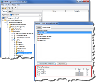
Figure 5.8-1 Granting access to the OLAP Schema
5.8.2 Member-Level Security
SAS Management Console provides an interface to assign member-level security per user to any member of the OLAP cube.
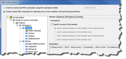
- Navigate to the specific OLAP cube by expanding the Authorization Manager and navigate from Resource Management > By Location > SASApp - OLAP Schema. Then navigate from the cube name to the dimension names and select the properties on a dimension where member-level security is required.

- On the Authorization tab, add the specific user or group that needs member-level security defined. The Add Authorization tab
 is greyed out. To access the Add Authorization tab, click the Grant Read check box
  to explicitly grant Read access (showing as checked with a white background). Explicit access removes any association with security definitions that are stated above this object in the security model, removing any inheritance between objects above this object and this one.

- After
clicking the Add
Authorization button, you can then specify what members the
users can view.
Note: If the cube requires that summarized data at all levels take the security settings into account, than a SECURITY_SUBSET option must be enabled.
At the first window of the cube designer, Cube Designer-General, clear the selection for Include secured member values in presummarized computations.
