
Measurement of porosity as a predictor of the transport properties of concrete
Abstract:
Fluid transport through concrete takes place almost entirely through the pores. The porosity is a measure of the total pore volume and does not take account of the connectivity or tortuosity of the pores, but it would still be expected to be a good predictor of transport. This chapter introduces different methods for measuring porosity and transport. The precise mechanism involved in a ‘vapour transport’ experiment is then discussed and relationships between porosity and transport are presented.
Key words
porosity; helium intrusion; mercury intrusion; oxygen permeability; vapour transport
8.1 Introduction
It is often easier and more reliable to measure the porosity of concrete and use it to predict the transport rather than to measure the transport properties directly. Fluid transport through concrete takes place almost entirely through the pores. This porosity can be measured directly with helium or mercury intrusion and calculated from weight loss on drying. These three measurements will give different results, and it is important to compare them before using them as predictors. A range of transport measurements are compared with porosities measured using these three methods. Chloride transport is considered in detail in Chapters 10–13, but a simple method is presented here to compare with porosity. Carbonation is controlled by the transport of atmospheric carbon dioxide into concrete and is thus an indirect measure of transport. Electrical resistivity is a measure of electromigration. A method for measuring oxygen transport is presented in detail. Finally, a method intended to measure water vapour transport is presented, but it is concluded that the samples were actually saturated during the test, indicating that the drying test presented in Chapter 7 would be preferred for this measurement.
8.2 Sample preparation and testing programme
8.2.1 Sample preparation
The mix designs are shown in Table 8.1. The silica fume (SF) was supplied by Elkem Chemicals from their works in Norway. The superplasticiser was a salt of napthalene formaldehyde condensate supplied by FEB (UK). The fine aggregate came from North Nottinghamshire and was a natural sand. The percentages given for superplasticiser were calculated from the quantities of solids which form 40 % of the solution as supplied. Mortar samples were made with the same proportions but without the coarse aggregate. Paste samples were made with the same proportions but without the coarse or fine aggregates.
Table 8.1
| Mix | A | B | C | D |
| SF/(PC + SF) | 0.20 | 0 | 0.20 | 0 |
| Water/(PC + SF) | 0.30 | 0.30 | 0.46 | 0.46 |
| Superplasticiser/(PC + SF) | 0.014 | 0.014 | 0.019 | 0.019 |
| Fine aggregate/(PC + SF) | 1.5 | 1.5 | 2.3 | 2.3 |
| Coarse aggregate (5–20 mm)/(PC + SF) | 3 | 3 | 4 | 4 |
| PC (kg/m3) | 344 | 430 | 252 | 315 |
| SF (kg/m3) | 86 | 0 | 63 | 0 |

The mortar samples were mixed in a Hobart mixer. The superplasticiser was mixed with the water and added to the sand and cement when they had already been mixed in a dry condition. Mixing continued for 2 min after a uniform consistency was observed. The highest speed of the mixer was used for the mixes with lower workability but, for those with highest workability, this caused them to be ejected from the mixer and a lower speed was used. The samples were cast in the appropriate moulds, kept covered in the laboratory for 24 h and then placed in the following curing conditions.
After casting, the samples were covered and kept at 20 °C for 24 h until they were struck. They were then cured using the three different curing conditions given in Table 8.2. The samples were tested at 3, 28 and 90 days. All combinations of the four mixes, three curing conditions and three test ages were used for the tests, giving a total of 36 ‘sample conditions’ which reflect a wide range of possible conditions for site concrete when first exposed to an aggressive environment.
Table 8.2
| Curing condition 1 (CC1) | 99 % RH, 20 °C |
| Curing condition 2 (CC2) | Treated with curing membrane and then stored at 70 % RH, 20 °C for 6 days and then in water at 6 °C |
| Curing condition 3 (CC3) | In water at 6 °C |
Different types of sample were used for the different tests as described below. No study was made of the surface properties of concrete, so for all samples used to measure transport properties samples were cut from the centres of the specimens and the outer surfaces were not tested. The temperature of 6 °C was chosen as being the lowest at which mixes of this type should be placed on a well managed site.
8.2.2 Sample testing programme
The tests that were carried out are summarised in Table 8.3. Compressive strength was measured because this is the property that is most often known for concrete mixes. The compressive strength was measured on 100 mm concrete cubes.
Table 8.3
| Test | Material |
| Porosity measurements | |
| Mercury intrusion | Paste |
| Helium intrusion | Paste/mortar/concrete |
| Weight loss | Paste/mortar/concrete |
| Transport property measurements | |
| Chloride transport | Concrete |
| Carbonation | Mortar |
| Oxygen transport | Mortar |
| Water vapour transport | Paste |
| Initial resistivity | Concrete |
| 28 day resistivity | Concrete |
| Other properties | |
| Compressive strength | Concrete |
8.3 Tests for porosity
8.3.1 Helium intrusion
The net volume of samples was measured by helium intrusion using a Micromeritics Autopycnometer 1320. This machine measures the volume of helium that a sample displaces (i.e. the net volume). The sample is positioned in one of two chambers which initially have equal volumes. After evacuation, an equal volume of helium is introduced into each chamber and the pressures are measured. The machine then calculated a volume change to the empty chamber to make the two volumes equal, i.e. to compensate for the presence of the sample. The volume change is effected with a piston and the helium is introduced again. The cycle repeats until equal pressures are found in both chambers at which time the volume of the sample is known from the position of the piston.
The samples were ground to pass a 1.18 mm sieve before testing to ensure full penetration into the pore structure. The samples were then weighed before testing and the specific gravity was calculated as the mass divided by the net volume. The dry density (DD, the mass divided by the bulk volume) was obtained from the weight loss measurements. The porosity was then obtained from equation (7.9).
The results are presented in Fig. 8.1. The consistent trends which may be observed in this figure indicate that the resolution of the measurements was adequate to differentiate the samples.

8.3.2 Mercury intrusion
Cylindrical samples of paste with a diameter of 25 mm and a length of approximately 15 mm were intruded using a Micromeritics Auto-Pore 9200 intrusion machine. In this technique, a small mortar sample is immersed in mercury in a glass container connected to a capillary tube with a conductive metallic coating. The entire container is then immersed in oil which is pressurised. As the pressure increases, the mercury is forced down the capillary tube and into the pores of the mortar. The volume entering the pores is measured as a change of electrical capacitance of the capillary tube. Mercury is used, despite its health risks, because of its high surface tension.
The machine had a maximum operating pressure of 414 MPa. The diameter of the pores was obtained using equation (8.1):
[8.1]
where:
r is the radius of the smallest pore that the mercury can enter
γ is the surface tension of the mercury
ɸ is the contact angle of the mercury with the pore surface and
P is the pressure.
The values used for the contact angle and the surface tension of the mercury were 130° and 0.484 N/m which give a minimum pore diameter of 0.003 μm at the highest pressure. Figure 8.2 shows a typical output from the mercury intrusion. In order to characterise the salient features of the intrusion curves for further analysis, the total intruded volumes in the pore size ranges in Table 8.4 were obtained from the experimental data. The recovery volume is the volume of mercury which came out of the samples when the pressure was released.

Table 8.4
| Range | Typical porosity |
| 10–170 μm | 0.5 % |
| 0.15–10 μm | 0.7 % |
| 0.01–0.15 μm | 16 % |
| 0.003–0.01 μm | 7 % |
| 0.003–10 μm (recovery) | 10 % |
These ranges are presented in Fig. 8.2 which shows the cumulative and differential intrusion volumes for two replicate samples with the size ranges marked with the vertical gridlines. For each range, the porosity was calculated as a percentage of the bulk volume of the samples.
8.3.3 Weight loss
For this purpose, samples were cast in disposable plastic cups. This method was used because the cups were convenient and did not require mould oil which would have affected the weight. The following weights were recorded:
2. wet (submerged) and surface dry weights after curing to give the density;
3. dry weights after drying to constant weight in a ventilated oven at 110 °C.
The Powers model was used to obtain the porosity as described in Section 7.3.3. These equations do not work for samples containing additional components such as SF. Attempts were made to extend the model using data from thermogravimetric analysis to determine the proportions of hydration products in the hydrated SF samples, but the porosities obtained were not consistent with other observations and are not reported here.
8.4 Tests for properties controlled by transport
8.4.1 Carbonation
Mortar samples measuring 25 mm by 25 mm by 200 mm long were exposed to an atmosphere of 90 % CO2 at a pressure of 1 bar at 21 °C and 70% relative humidity (RH). The apparatus for this experiment was complicated by the need to extract moisture arising from the reaction. The shrinkage was measured at 18 days after exposure with a comparator using a linear voltage displacement transducer (LVDT). The recorded strain was a total arising both from the carbonation and from drying shrinkage while in the carbonation chamber.
8.4.2 Resistivity
Concrete samples 75 mm diameter by 220 mm long were cast with a 12 mm diameter steel bar 225 mm long positioned centrally and projecting 50 mm from one end and thus having 45 mm cover at the other end. The samples were cast upside down by locating the steel bar in a wooden block in the base of a cylinder mould. They were then immersed in salt-saturated water to a depth of 190 mm (i.e. with 30 mm of concrete clear of the solution). A circuit was then formed between the steel bar and a mild steel secondary electrode in the salt solution. The chloride was driven into the concrete by electromigration by applying a negative voltage to the secondary electrode at 100 mV relative to a saturated calomel reference electrode in the solution for up to 28 days using a potentiostat.
To measure resistivity, the potentiostat was disconnected and an alternating voltage of 100 mV at 50 Hz was applied to the circuit and the current was measured. These samples were also used for corrosion tests reported in Chapter 13 but, by using alternating current, the readings of resistivity were not affected by corrosion of the bar.
8.4.3 Chloride transport
Concrete beams were cast measuring 500 mm long by 100 mm square. A rebate 20 mm deep by 40 mm wide by 300 mm long was formed in the top of each beam and, after curing, four 32 mm diameter holes were drilled to a depth of approximately 10 mm in the bottom of the rebate using a heavy rotary hammer drill. The rebate was then filled with saturated salt solution and the samples kept at approximately 20 °C. After 28 days, samples were drilled from the bottom of the holes and tested for acid soluble chloride by titration. The procedure was:
1. remove salt solution and wash off remaining salt;
2. permit to dry at room temperature;
3. drill for 10 s and discard dust;
4. drill for 5 s and retain dust as sample 1 (approx. 5 mm depth);
5. drill for 5 s and discard dust;
6. drill for 5 s and retain dust as sample 2 (approx. 10 mm depth).
The depth of the sampling was calculated by weighing the samples and checked by measurement with a caliper. The results were obtained by fitting an exponential decay function to the two readings and integrating.
The transport in this test will have been substantially affected by ion–ion interactions as discussed in Chapter 10 so no attempt was made to obtain diffusion coefficients using Fick’s law.
8.5 Oxygen transport
8.5.1 Apparatus
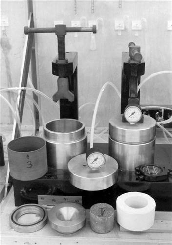
Sections (20 mm long) of 25 mm mortar cores were tested for oxygen transport under an applied pressure difference of 1 and 2 bar. The rate of flow was measured with a bubble flow meter. The apparatus is shown in Fig. 8.3. The seal is formed by first coating the curved surface of the sample with silicone rubber and then compressing it into a surround of synthetic rubber.
8.5.2 Preparation of the samples
Mortar samples were cast as 100 mm cubes. When they were struck, the 25 mm cores were cut from them and 20 mm long samples were cut from the central portion of the cores. At the test age, the samples were dried for 24 h and at 105 °C and placed in a desiccator. When they had cooled, a thin film of silicone rubber was applied to the curved surfaces and allowed to set for 24 h before testing.
Before testing the CC2 samples, any remaining curing agent on the end surfaces was removed using no. 40 grit sandpaper. Penetration of this material into the pores could, however, have reduced the flow rates, but inspection of the samples indicated that this would not have been significant.
8.5.3 Testing procedure
The samples were tested at applied oxygen pressures of 1 and 2 atm above ambient. Two samples were tested for each condition. Before testing, the samples were allowed a minimum of 30 min to equilibrate and to purge the air from the system and, for samples with very low flow rates, this was increased to several hours. Two readings were taken on each sample at each pressure and the average of these two readings was used. Different diameter bubble flow meters were used, ranging from 1.7 mm for very low flows to 10 mm for high flows.
Leakage was checked using some spare samples; these were spread with silicone rubber over the flat surfaces as well as the curved surface and checked for gas flow. No flow was observed. If there had been any substantial leakage, the range of the data would have been increased.
8.5.4 Calculation of the coefficient of permeability
The general equations for pressure-driven flow from Section 1.2.1 are used and the analysis is similar to that in Section 4.5. If Q is the volume per second passing through the sample measured at the low pressure P1 (assuming an ideal gas):
[8.2]
where:
A is the cross-sectional area of the sample and
P1 is the low pressure (i.e. the pressure on the outlet side of the sample, this is atmospheric pressure in this work).
Thus:
[8.3]
and:
[8.4]
Integrating across the sample:
[8.5]
 [8.5]
[8.5]
where:
P2 is the high pressure (i.e. the pressure on the input side of the sample) and
X is the sample thickness.
Thus:
[8.6]
 [8.6]
[8.6]
The viscosity of oxygen gas e = 2.02 × 10⁻⁵ Ns/m2 and P1 = 1 atm = 0.101 MPa.
8.5.5 Relationship between readings at different pressures
The relationship between the readings at the two pressures is shown in Fig. 8.4 which is plotted logarithmically to spread the readings. It may be seen that the data lie very accurately on the line of equality, indicating that the use of Darcy’s equation was justified and Knudsen flow was not significant. The average of the two readings was calculated and is plotted in Fig. 8.5.


8.6 Vapour transport
8.6.1 Preparation of the samples
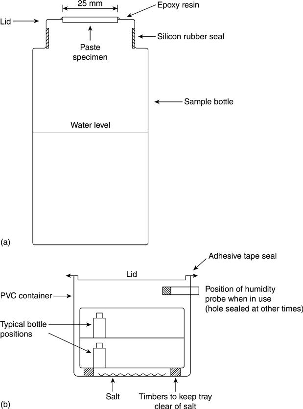
Paste samples for measurement of water vapour transport were cast as 100 mm cubes, and 25 mm diameter cores were cut from them before curing. At the test age, thin discs were cut from the central portion of the cores. The thickness of each disc was measured with a micrometer. The thickness of all the discs fell in the range 3.5–4.7 mm. The discs were permitted to dry at room temperature for approximately 2 h and then set in epoxy resin in holes formed in the lids of 125 cc sample bottles. The bottles were then part filled with de-ionised water and the lids put on them and sealed as shown in Fig. 8.6. The effectiveness of the seals was checked by briefly inverting the bottles. the bottles were then placed in trays in large storage containers. Details of the environmental conditions in the containers were:
| Container 1: | Open to the atmosphere in a room controlled at 70 % RH. |
| Container 2: | Sealed with a quantity of sodium dichromate in the bottom to give an RH of 55.2 %. |
| Container 3: | Sealed with a quantity of lithium chloride to give an RH of 12.4 %. |
All of the containers were kept at 21 °C. The RH was checked periodically using an electronic probe. The water transmission rate was measured by weighing the bottles. Two samples were tested for each of the four mixes, three curing conditions, three test ages and three containers to give a total of 216 bottles.
8.6.2 Blank tests
In addition to the sets of cementitious samples, a number of blank samples (coins) were tested. No measurable weight loss occurred, and this confirmed that the bottles and seals were impermeable and the only transmission path was through the samples.
8.6.3 Analysis of the data
Initial preparation
The weights of the bottles were initially plotted against time. A typical plot showing results of six samples is shown in Fig. 8.7. These plots were used to identify bottles where obvious leakage was causing a wrong result. Out of the total of 216 bottles, there were three of this type and the results from them were not used.

Interpretation of the data
It may be seen from Fig. 8.6 that the initial mass loss rate is higher than the steady state. The following two processes are believed to contribute to this effect.
1. When the samples were first installed they had a relatively constant moisture content throughout. Whatever the final distribution, it was certainly not constant across the thickness. An increase in moisture content on the wet side would not affect the measured weight, but a loss from the dry side would cause a loss of weight. The factors controlling the exact rate of moisture loss are complex because the rate of migration of water will depend on the local humidity gradient, and the total amount to be lost from any given depth will depend on the final distribution. As a rough approximation it is, however, reasonable to assume an exponential decay, i.e. the rate of loss will be proportional to the amount remaining to be lost.
2. When the samples were installed they were not fully hydrated. Due to the presence of moisture, the hydration will have continued and the hydration products will have formed in previously open pores. The factors controlling the transmission rate are again complex because the rate of hydration will depend on the availability of water. An exponential decay may be very approximately justified by assuming that the rate of hydration depends on the quantity of cement remaining to hydrate, and the rate of transmission decreases linearly with the quantity of hydration products present. Thus the rate of hydration will decay exponentially and the rate of transmission will follow it.
If the two processes are assumed to proceed at approximately the same speed they may be represented by a single term to describe the initial additional losses, i.e. M0e−Kt where K is a rate constant to represent the effect of both processes. Thus:
[8.7]
where:
M is the cumulative mass loss to current time t and
M0 + Ct is the linear long term mass loss.
This equation was fitted to each set of results and thus, for each sample, the constant C represents the steady state loss and the constants M0 and K show the extent and duration of the initial additional losses. These values are shown in Table 8.5 for the experimental results shown in Fig. 8.7.
Table 8.5
Values of the constants of equation (8.7)
| Test age (days) | Sample no. | Constants | ||
| C | M0 | K | ||
| 3 | 1 | 0.026 | 1.186 | 0.056 |
| 3 | 2 | 0.024 | 1.240 | 0.055 |
| 28 | 1 | 0.019 | 0.784 | 0.067 |
| 28 | 2 | 0.019 | 0.689 | 0.061 |
| 90 | 1 | 0.016 | 0.545 | 0.131 |
| 90 | 2 | 0.015 | 0.547 | 0.155 |

Effect of sample thickness
The dependence on thickness in the data was checked by considering each similar pair of samples. For each pair, the percentage difference in thickness and the percentage difference in the constants C, M and K were calculated. No correlation was found between any of the constants and the thickness, and it was thus concluded that the rate is independent of thickness.
Effect of relative humidity (vapour pressure difference)
The dependence of the measured weight losses on RH was investigated by plotting the relationship between the results from the samples exposed to different environments (Fig. 8.8). It may be seen that there are clear linear relationships between the results from the different environments, i.e. different relative humidities.
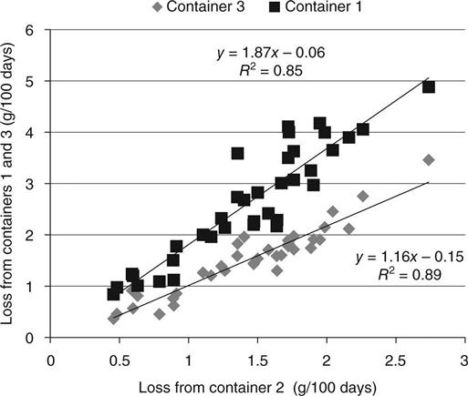
The target RH for container 1 was 70 % and for container 2 it was 55.2 %, and thus a linear dependence of rate on RH would give a ratio of (100 − 55.2)/100 − 70) = 1.49. If Darcy’s law is applied, equation (8.6) shows that each of the terms is squared and this gives a ratio of 1.36. The other ratios are in Table 8.6.
Table 8.6
Effect of relative humidity on weight loss
| Container | Ratio of RH drop | Darcy ratio | Observed C ratio |
| 2/1 | 1.49 | 1.36 | 0.95 (0.88) |
| 3/2 | 1.95 | 1.41 | 1.83 (0.85) |
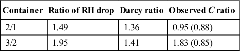
Note: figures in brackets after the ratios are the values of R2 for the relationship.
The data indicates that the losses from container 1 were higher than expected because of increased air circulation (container 1 was open, but containers 2 and 3 were closed). The relationship between containers 2 and 3 shows a direct dependence on RH more than a Darcy relationship.
An average of the results for the three containers was obtained after multiplying the results from containers 1 and 3 by a constant factor to give each set the same mean value in order to give equal weighting. The average is plotted in Fig. 8.9.

8.7 Results and discussion
Two readings were obtained for each sample condition for each experiment. The average of each pair of readings was used for the analysis reported here.
The relationships between all of the different variables studied (data columns) were calculated as the correlation coefficient R2. The value of this for 1 % significance is 0.17 for the Portland cement (PC) and SF samples together (a complete column of 36 values) and 0.31 for the PC or the SF samples individually (half a column – 18 values) (see for example Tables 8.7 and 8.8).
Table 8.7
Comparison of correlations (values of R2) for paste, mortar and concrete for chloride transport and strength
| Predictor | Type of sample | Property | |
| Chloride transport | Strength | ||
| Measurements of porosity from helium intrusion (all samples) | Paste | 0.537 | 0.671 |
| Mortar | 0.376 | 0.295 | |
| Concrete | 0.593 | 0.450 | |
| Calculations of porosity from weight loss (PC samples only) | Paste | 0.756 | 0.944 |
| Mortar | 0.045 | 0.006 | |
| Concrete | 0.646 | 0.884 | |

Table 8.8
| Property | Predictor | All | PC | SF |
| Chloride concentration | Paste porosity (helium) | 0.537 | 0.730 | 0.661 |
| Concrete porosity (helium) | 0.593 | 0.702 | 0.257 | |
| Paste porosity (mercury) | 0.771 | 0.808 | 0.716 | |
| Calculated paste porosity | 0.756 | |||
| Calculated concrete porosity | 0.646 | |||
| Carbonation strain microstrain | Paste porosity (helium) | 0.652 | 0.717 | 0.717 |
| Concrete porosity (helium) | 0.458 | 0.719 | 0.617 | |
| Paste porosity (mercury) | 0.625 | 0.788 | 0.698 | |
| Calculated paste porosity | 0.615 | |||
| Calculated concrete porosity | 0.700 | |||
| Log of oxygen permeability (m2 × 10−18) | Paste porosity (helium) | 0.448 | 0.700 | 0.424 |
| Concrete porosity (helium) | 0.645 | 0.743 | 0.428 | |
| Paste porosity (mercury) | 0.634 | 0.807 | 0.374 | |
| Calculated paste porosity | 0.741 | |||
| Calculated concrete porosity | 0.743 | |||
| Water vapour transport | Paste porosity (helium) | 0.807 | 0.765 | 0.922 |
| Concrete porosity (helium) | 0.334 | 0.613 | 0.703 | |
| Paste porosity (mercury) | 0.600 | 0.699 | 0.903 | |
| Calculated paste porosity | 0.574 | |||
| Calculated concrete porosity | 0.516 | |||
| Inverse of cube strength (N/mm2) | Paste porosity (helium) | 0.671 | 0.861 | 0.602 |
| Concrete porosity (helium) | 0.450 | 0.901 | 0.157 | |
| Paste porosity (mercury) | 0.780 | 0.941 | 0.683 | |
| Calculated paste porosity | 0.944 | |||
| Calculated concrete porosity | 0.884 | |||
| Log of initial resistance (Ω) | Paste porosity (helium) | 0.208 | 0.741 | 0.294 |
| Concrete porosity (helium) | 0.232 | 0.726 | 0.228 | |
| Paste porosity (mercury) | 0.279 | 0.769 | 0.301 | |
| Calculated paste porosity | 0.813 | |||
| Calculated concrete porosity | 0.613 | |||
| Log of 28 day resistance (Ω) | Paste porosity (helium) | 0.276 | 0.701 | 0.808 |
| Concrete porosity (helium) | 0.589 | 0.763 | 0.669 | |
| Paste porosity (mercury) | 0.532 | 0.801 | 0.753 | |
| Calculated paste porosity | 0.850 | |||
| Calculated concrete porosity | 0.632 |

8.7.1 The mechanisms of oxygen and vapour transport
The experiments indicate that the transmission of oxygen is adequately described by the Darcy equation. The mechanism of transmission of water vapour is clearly different. This difference is shown very clearly in Fig. 8.10 where the results of oxygen transmission are plotted against vapour transmission and the log of the oxygen permeability has similar range to the water transmission measurements. The observation that the water transmission rate is independent of the sample thickness severely limits the choice of possible mechanisms. The possibility of a continuously changing moisture content across the thickness consistent with a Darcy relationship is ruled out. Typical values of mean free path are given in Table 6.4 and are in the range of 0.1 μm; however, Table 8.4 shows typical pore diameters of 0.01 μm or below. The mean free path of a molecule of water vapour at room temperature is many times greater than the size of continuous pores in concrete and the Kelvin equation (3.1) shows that at 96 % RH pores with diameters below 35 μm will sustain a meniscus. It may therefore be concluded that, with the exception of an outer surface layer, the pores are all either full of water or vapour at near 100 % RH. This model would indicate that keeping one side at 100 % RH would make the transmission rate independent of thickness.

Further support for the theory that this is not a vapour diffusion process is gained from the observation of water droplets on the underside of the samples. These droplets will clearly prevent the ingress of any gas or vapour into the sample. Rose (1965) discussed the various degrees of saturation possible in a porous body. He suggests two mechanisms of transmission without full saturation, but without a vapour pressure gradient. One takes place when just the necks of the pores are filled with water, where vapour condenses on one side of the neck and evaporates from the other. The other mechanism is surface creep of a fine film of water coating the pore surfaces.
Powers (1960) proposed a mechanism for the loss of water from the dry side. He observed that if it was necessary for water to evaporate from surfaces in the necks of the outer pores as in the ‘ink bottle’ analogy, virtually no water would be lost. He therefore proposed a mechanism where the process is controlled by the formation of vapour bubbles in those pores at the surface which are of adequate size. The total areas which will be intersected by a cut through a sample will form the same fraction of the cut surface area as the fraction of the sample volume occupied by the pores, i.e. the porosity. This would indicate that the rate would be linearly dependent on porosity which may be seen to be a measure of a surface as well as bulk property. The relationship is shown in Fig. 8.11, and it can be seen that the line is an excellent fit (R2 = 0.81), but it does not pass through the origin (for the steady state, 90 day porosity values were used). The data indicates that at porosity 11 %, the pores become either discontinuous or too small for bubble formation and the transmission stops.

8.7.2 The effect of test age
It may be seen from Figs 8.1 and 8.9 that the vapour transport and porosity decrease with increasing maturity as expected. Figure 8.5, however, shows the oxygen permeability increasing with time for the SF samples from CC1 (moist cure at 20 °C). It is possible that this could have been caused by open porosity caused by the depletion of lime during the progress of the pozzolanic reaction, but the absence of this effect in the dry cure samples (CC2) indicates that it was caused by cracking as a result of the drying procedure on the SF samples. It is therefore indicated that the conditions most likely to produce samples which are virtually impermeable to oxygen in normal environments are prolonged moist curing of SF samples with low water to cement (w/c) ratios.
8.7.3 The relative importance of the measurements of oxygen and vapour permeability
The results from the vapour transmission experiment have been presented in units of weight loss because the permeability model used for the oxygen results was not correct for the physical process. If the equations are used, however, to obtain an estimate of the relative effect of the two processes, the permeability coefficients in m2 are equal to 7 × 10⁻¹⁶ times the weight loss in g/100 day. This calculation assumes that the transmission of water is by pure vapour permeation and should therefore be treated with considerable caution. A value of 10−5 has been used for the viscosity of water vapour. Using this factor, the measured water permeabilities lie in the range of 2 × 10⁻¹⁵–4 × 10⁻¹⁶ while the oxygen permeabilities lie in the range of 10−15–10−21. These results imply that the transport rates of water and oxygen in the control mixes are similar, but the use of the SF with a low w/c ratio (mix A) could cause the permeability to oxygen to become significantly lower than that for water. The major increase in the sensitivity to different curing regimes shown in Figure 8.5 is, however, a cause for concern if this property is to be used. In particular, the increase in permeability with curing time for both SF mixes in CC1 (20 °C) is of interest.
The observed sensitivity of the water vapour transport rates to the different curing conditions will have been reduced by the effect of continuing hydration during the experiments.
8.7.4 The effect of water vapour on the oxygen permeability
All of the samples tested for oxygen permeability in this work were dried before testing. Measuring gas permeabilities at other humidities is difficult because both the samples and the gas to be permeated through them must be equilibrated to the required humidity at the start of the test and the entire system must be sealed from the atmosphere during the test to prevent drying. Results from experiments of this type are presented in Chapter 6 and show the permeability of a grout falling from 3 × 10⁻¹⁶ when dry to 3 × 10⁻¹⁸ at 75 % RH and to below 10−21 at close to 100 % RH. If a similar effect was observed with samples of mix A where the permeability is already low, the effect would create an almost impermeable barrier to oxygen.
8.7.5 Comparison between different measurements of paste porosity
Comparison between the different test methods
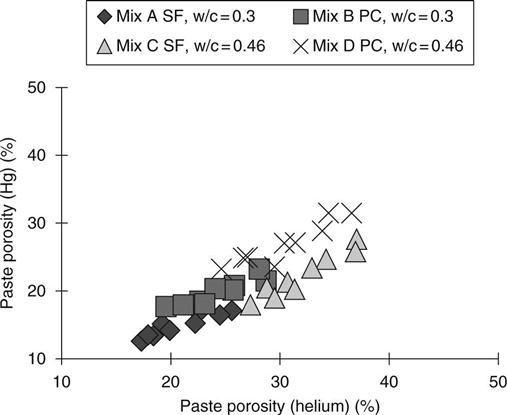
The relationship between the different measurements is shown in Figs 8.12 and 8.13. Comparisons could only be made for paste because these were the only type used for mercury intrusion. From Fig. 8.12 it may be seen that mercury intrusion yields a lower value than helium intrusion. This would be expected because the samples were ground for helium intrusion and the low molecular size and viscosity of the helium. The calculations of porosity were only used for the PC samples, but Fig. 8.13 shows that these samples correlate well, with the helium results giving generally slightly lower values.

Porosities for different pore size ranges
The porosity from mercury intrusion was, as described above, subdivided into porosities for different pore size ranges. These porosities in the different pore size ranges were correlated with the total porosities also obtained from mercury intrusion. No correlation was observed in the size range for the largest pores.
The correlation between porosities in the 0.15–10 μm range and total porosity was negative (Fig. 8.14). Significance values of R2 of 0.314 for the SF samples and 0.340 for all of the samples were obtained. The negative correlation indicates that the porosity in this range, which increases with a decrease in total porosity, is unlikely to be significant in predictive models for properties which generally correlate with porosity.

The bulk of the pores lie in the 0.01–0.15 μm range and a good correlation with the total porosity was expected. Figure 8.15 shows, however, that the SF samples had significantly lower porosity in this range and the relationship with total porosity was therefore different from that for the PC mixes.

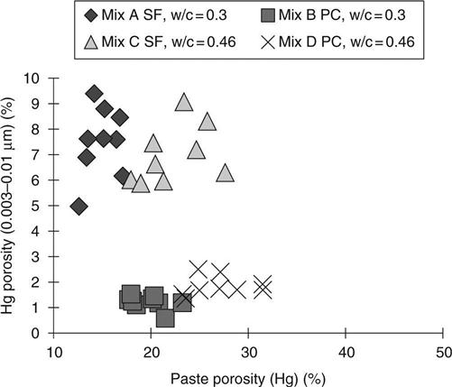
Figure 8.16 for the 0.003–0.01 μmrange showsthe extent ofthe refinement of the pore structure caused by the SF. The correlations with total porosity are not significant, but the effect of the SF is very clear. This refinement of the pore structure has the effect of reducing the recovery volumes for the SF samples. This may be seen in Fig. 8.17.

8.7.6 Measurements from concrete, mortar or paste
For the helium intrusion and the weight loss measurements, tests were carried out on concrete, mortar and paste samples. When considering which of these to use as predictors for concrete properties, there are two conflicting factors: measurements on concrete are theoretically the most realistic, but concrete porosities are lower than those for mortar and paste so the accuracy of measurement will be lower. It is obviously possible to calculate one porosity from another with a knowledge of the proportions and porosity (if any) of the aggregate. Table 8.7 shows some of the correlations of porosities with properties that were measured.
It may be seen that the mortar results generally gave poorer correlations, but neither the concrete or the paste was found to be universally better. The correlations for paste and concrete porosity for all of the measured properties are shown in Table 8.8 and are discussed in subsequent sections.
8.7.7 Pore size ranges in mercury intrusion
For the main transport properties, attempts were made to develop multiple regression models based on the porosities from different pore size ranges obtained from mercury intrusion. It was hoped that the different characteristics of the pore size distributions would combine in linear combinations to form a predictive model. It was found, however, that in each case a single predictor model based on the total porosity could not be improved by including any of the individual pore size ranges. This might be expected from the negative correlation between total porosity and some of the porosities in size ranges.
8.7.8 Chloride transport
The relationship between chloride concentration and paste porosity measured by mercury intrusion is shown in Fig. 8.18. The measured chloride concentration will be proportional to the chloride transport to the point of measurement. It may be seen that the porosity measurement works as an excellent predictor and the correlation coefficient is 0.77. If the porosity from helium intrusion is used (Fig. 8.19), it may be seen that the transport would be over-estimated for mix C, which is the SF mix with the higher w/c ratio. Looking at the relationship between the mercury and helium porosities (Fig. 8.12), it may be seen that mix C has a higher than expected porosity from the helium intrusion. It is concluded from these observations that mix C has a substantial closed porosity which was not accessed by the mercury because the samples were not ground before the mercury test and because of the higher viscosity of the mercury. This closed porosity would not contribute to the chloride transport.


For the PC samples alone, all three different methods of measuring porosity gave high correlations of porosity with chloride concentration in the range 0.65–0.8.
8.7.9 Carbonation
The relationships between carbonation strain and helium and mercury porosity are similar (Figs 8.20 and 8.21). The helium porosity shows a slightly higher correlation (see Table 8.8), but both measurements may be taken as equally good predictors of carbonation.


8.7.10 Oxygen transport
The observed values of oxygen permeability had a range of several orders of magnitude, and none of the measured porosities were good predictors for them. It was found, however, that the log of the oxygen permeability could be predicted with porosity. For the PC samples, all of the measurements of porosity gave R2 in the range 0.7–0.8. For the SF, the correlations are far lower, and the reason for this may be seen from Fig. 8.22 which shows the relationship with the porosity from mercury intrusion. It may be seen that there are some SF samples which had low porosity but high permeability giving an apparent decrease in permeability with increasing porosity for the lower porosity samples of mixes A and C. This might have been caused by the creation of a connected pore system when the calcium hydroxide is depleted by the pozzolanic reaction, but there is no other evidence to support this explanation and micro-cracking of the higher strength samples during drying is probably more likely.

8.7.11 Water vapour transport
It was shown in Section 8.12.1 that, in the experiments that were carried out, the water vapour transport rate was controlled by the rate of evaporation from the low humidity side of the sample. This rate of evaporation will depend on the surface area of the pores exposed on the surface and this area will, in turn, depend on the total porosity. It may be seen that, as expected from this, the correlation is highest with the helium intrusion. Looking at the relationships in Figs 8.23 and 8.24, it is apparent that mix D is the cause of the poorer relationship with mercury intrusion results. This will be because all of the other mixes have a higher proportion of closed porosity.


8.7.12 Cube strength
In order to obtain a good predictive model, the inverse of the cube strength was used. The relationship with the calculated paste porosity was excellent (for PC samples only). In this case, the strength is likely to be used as the predictor for porosity, and the relationship with mercury porosity may be seen in Fig. 8.25.

8.7.13 Resistivity
In order to obtain better predictions, the log of the resistance values was used in all cases. The relationship between porosity and initial resistance is clearest in fig. 8.26, giving the results from helium intrusion. The PC results and the SF results from tests at age 3 days all lie on a clear line, and the 28 day results from cold curing (CC3) also lie on this line. The other SF samples lie above the line. This increase in resistance has been caused by the depletion of lime by the pozzolanic reaction and is independent of porosity (Cabrera and Claisse, 1991). After 28 days of anodic polarisation, all of the SF samples have high resistivity due to lime depletion and lie on a separate clear line (Fig. 8.27). Because all of the resistance samples were the same size, the resistivity values for the materials will be proportional to the measured resistances.


8.8 Conclusions
• Transport of oxygen through dry cementitious samples is accurately described by the Darcy equation, and the measured permeabilities vary over a substantial range of values.
• The rate of transport of water vapour was not found to vary greatly for the different samples and was proportional to the porosities of the samples.
• The results indicate that under the correct conditions SF could be used to make a material which is almost impermeable to oxygen.
• When using measurements of porosity as predictors for bulk concrete properties, it was equally valid to use measurements on paste or concrete samples.
• The models using total porosity to predict the performance of the concrete could not be improved by including data for the individual pore size ranges from mercury intrusion.
• Mercury intrusion was the best predictor of chloride transport because the mercury does not penetrate closed porosity and this closed porosity does not contribute to the transport.
• Helium intrusion was the best predictor of water vapour transport if it is controlled by evaporation because it will depend on the total porosity.
• The resistivity of concrete was predicted well by porosity models but, for mixes containing SF, the effect of lime depletion by the pozzolanic reaction is more significant.