We will write a series of Python statements manipulating arrays and matrices, and learn how to use NumPy on the way. Our intent is to get you used to working with NumPy arrays, as NumPy will serve as the basis for most of the recipes in this book.

Let's start by creating some simple matrices and arrays:

#Recipe_1a.py
# Importing numpy as np
import numpy as np
# Creating arrays
a_list = [1,2,3]
an_array = np.array(a_list)
# Specify the datatype
an_array = np.array(a_list,dtype=float)


# Creating matrices
a_listoflist = [[1,2,3],[5,6,7],[8,9,10]]
a_matrix = np.matrix(a_listoflist,dtype=float)

Now we will write a small convenience function in order to inspect our NumPy objects:

#Recipe_1b.py
# A simple function to examine given numpy object 
def display_shape(a):
    print 
    print a
    print
    print "Nuber of elements in a = %d"%(a.size)
    print "Number of dimensions in a = %d"%(a.ndim)
    print "Rows and Columns in a ",a.shape
    print 

display_shape(a_matrix)

Let's see some alternate ways of creating arrays:

#Recipe_1c.py
# Alternate ways of creating arrays
# 1. Leverage np.arange to create numpy array
created_array = np.arange(1,10,dtype=float)
display_shape(created_array)

# 2. Using np.linspace to create numpy array
created_array = np.linspace(1,10)
display_shape(created_array)

# 3. Create numpy arrays in using np.logspace
created_array = np.logspace(1,10,base=10.0)
display_shape(created_array)

# Specify step size in arange while creating
# an array. This is where it is different
# from np.linspace
created_array = np.arange(1,10,2,dtype=int)
display_shape(created_array)

We will now look at the creation of some special matrices:

#Recipe_1d.py
# Create a matrix will all elements as 1
ones_matrix = np.ones((3,3))
display_shape(ones_matrix)
# Create a matrix with all elements as 0
zeros_matrix = np.zeros((3,3))
display_shape(zeros_matrix)

# Identity matrix
# k parameter  controls the index of 1
# if k =0, (0,0),(1,1,),(2,2) cell values
# are set to 1 in a 3 x 3 matrix
identity_matrix = np.eye(N=3,M=3,k=0)
display_shape(identity_matrix)
identity_matrix = np.eye(N=3,k=1)
display_shape(identity_matrix)

Armed with the knowledge of array and matrix creation, let's see some shaping operations:

Recipe_1e.py
# Array shaping
a_matrix = np.arange(9).reshape(3,3)
display_shape(a_matrix)
.
.
.
display_shape(back_array)

Now, proceed to see some matrix operations:

#Recipe_1f.py
# Matrix operations
a_matrix = np.arange(9).reshape(3,3)
b_matrix = np.arange(9).reshape(3,3)
.
.
.
print "f_matrix, row sum",f_matrix.sum(axis=1)

Finally, let's see some reverse, copy, and grid operations:

#Recipe_1g.py
# reversing elements
display_shape(f_matrix[::-1])
.
.
.
zz = zz.flatten()

Let's look at some random number generation routines in the NumPy library:

#Recipe_1h.py
# Random numbers
general_random_numbers = np.random.randint(1,100, size=10)
print general_random_numbers
.
.
.
uniform_rnd_numbers = np.random.normal(loc=0.2,scale=0.2,size=(3,3))

Let's start by including the NumPy library:

# Importing numpy as np
import numpy as np

Let's proceed with looking at the various ways in which we can create an array in NumPy:

# Arrays
a_list = [1,2,3]
an_array = np.array(a_list)
# Specify the datatype
an_array = np.array(a_list,dtype=float)

An array can be created from a list. In the preceding example, we declared a list of three elements. We can then use np.array() to convert the list to a NumPy one-dimensional array.

The datatype can also be specified, as seen in the last line of the preceding code:

We will now move from arrays to matrices:

# Matrices
a_listoflist = [[1,2,3],[5,6,7],[8,9,10]]
a_matrix = np.matrix(a_listoflist,dtype=float)

We will create a matrix from a listoflist. Once again, we can specify the datatype.

Before we move further, we will define a display_shape function. We will use this function frequently further on:

def display_shape(a):
    print 
    print a
    print
    print "Nuber of elements in a = %d"%(a.size)
    print "Number of dimensions in a = %d"%(a.ndim)
    print "Rows and Columns in a ",a.shape
    print

Every NumPy object has the following three properties:

size: The number of elements in the given NumPy object

ndim: The number of dimensions

shape: The shape returns a tuple with the dimensions of the object

This function prints out all the three properties in addition to printing the original element.

Let's call this function with the matrix that we created previously:

display_shape(a_matrix)

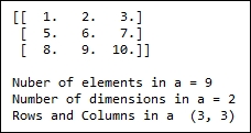
As you can see, our matrix has nine elements in it, and there are two dimensions. Finally, we can see the shape displays both the dimensions and number of elements in each dimension. In this case, we have a matrix with three rows and three columns.

Let's now see a couple of other ways of creating arrays:

created_array = np.arange(1,10,dtype=float)
display_shape(created_array)

The NumPy arrange function returns evenly spaced values in the given interval. In this case, we want an evenly spaced number between 1 and 10. Refer to the following link for more information about arange:

http://docs.scipy.org/doc/numpy/reference/generated/numpy.arange.html

# An alternate way to create array
created_array = np.linspace(1,10)
display_shape(created_array)

NumPy's linspace is similar to arrange. The difference is how we will request the number of samples that are required. With linspace, we can say how many elements we need between the given range. By default, it returns 50 elements. However, in arange, we will need to specify the step size:

created_array = np.logspace(1,10,base=10.0)
display_shape(created_array)

NumPy provides you with several functions to create special types of arrays:

ones_matrix = np.ones((3,3))
display_shape(ones_matrix)

# Create a matrix with all elements as 0
zeros_matrix = np.zeros((3,3))
display_shape(zeros_matrix)

The ones() and zeros() functions are used to create a matrix with 1 and 0 respectively:

Identity that the matrices are created, as follows:

identity_matrix = np.eye(N=3,M=3,k=0)
display_shape(identity_matrix)

The k parameter controls the index where value 1 has to start:

identity_matrix = np.eye(N=3,k=1)
display_shape(identity_matrix)

The shape of the arrays can be controlled by the reshape function:

# Array shaping
a_matrix = np.arange(9).reshape(3,3)
display_shape(a_matrix)

By passing -1, we can reshape the array to as many dimensions as needed:

# Paramter -1 refers to as many as dimension needed
back_to_array = a_matrix.reshape(-1)
display_shape(back_to_array)

The ravel and flatten functions can be used to convert a matrix to a one-dimensional array:

a_matrix = np.arange(9).reshape(3,3)
back_array = np.ravel(a_matrix)
display_shape(back_array)

a_matrix = np.arange(9).reshape(3,3)
back_array = a_matrix.flatten()
display_shape(back_array)

Let's look at some matrix operations, such as addition:

c_matrix = a_matrix + b_matrix

We will also look at element-wise multiplication:

d_matrix = a_matrix * b_matrix

The following code shows a matrix multiplication operation:

e_matrix = np.dot(a_matrix,b_matrix)

Finally, we will transpose a matrix:

f_matrix = e_matrix.T

The min and max functions can be used to find the minimum and maximum elements in a matrix. The sum function can be used to find the sum of the rows or columns in a matrix:

print
print "f_matrix,minimum = %d"%(f_matrix.min())
print "f_matrix,maximum = %d"%(f_matrix.max())
print "f_matrix, col sum",f_matrix.sum(axis=0)
print "f_matrix, row sum",f_matrix.sum(axis=1)

The elements of a matrix can be reversed in the following way:

# reversing elements
display_shape(f_matrix[::-1])

The copy function can be used to copy a matrix, as follows:

# Like python all elements are used by reference
# if copy is needed copy() command is used
f_copy = f_matrix.copy()

Finally, let's look at the mgrid functionality:

# Grid commands
xx,yy,zz = np.mgrid[0:3,0:3,0:3]
xx = xx.flatten()
yy = yy.flatten()
zz = zz.flatten()

The mgrid functionality can be used to get the coordinates in the m-dimension. In the preceding example, we have three dimensions. In each dimension, our values range from 0 to 3. Let us print xx, yy, and zz to understand a bit more:

Let's see the first element of each array. [0,0,0] is the first coordinate in our three-dimensional space. The second element in all three arrays, [0,0,1] is another point in our space. Similarly, using mgrid, we captured all the points in our three-dimensional coordinate system.

NumPy provides us with a module called random in order to give routines, which can be used to generate random numbers. Let's look at some examples of random number generation:

# Random numbers
general_random_numbers = np.random.randint(1,100, size=10)
print general_random_numbers

Using the randint function in the random module, we can generate random integer numbers. We can pass the start, end, and size parameters. In our case, our start is 1, our end is 100, and our size is 10. We want 10 random integers between 1 and 100. Let's look at the output that is returned:

Random numbers from other distributions can also be produced. Let's see an example where we get 10 random numbers from a normal distribution:

uniform_rnd_numbers = np.random.normal(loc=0.2,scale=0.2,size=10)
print uniform_rnd_numbers

Using the normal function, we will generate a random sample from a normal distribution. The mean and standard deviation parameters of the normal distribution are specified by the loc and scale parameters. Finally, size determines the number of samples.

By passing a tuple with the row and column values, we can generate a random matrix as well:

uniform_rnd_numbers = np.random.normal(loc=0.2,scale=0.2,size=(3,3))

In the preceding example, we generated a 3 x 3 matrix, which is shown in the following code:

You can refer to the following link for some excellent NumPy documentation:

http://www.numpy.org/