
Let us recall the Boosting algorithm explained in the previous recipe. In boosting, we fitted an additive model in a forward, stage-wise manner. We built the classifiers sequentially. After building each classifier, we estimated the weight/importance of the classifiers. Based on weights/importance, we adjusted the weights of the instances in our training set. Misclassified instances were weighted higher than the correctly classified ones. We would like the next model to pick those incorrectly classified instances and train on them. Instances from the dataset which didn't fit properly were identified using these weights. Another way of looking at it is that those records were the shortcomings of the previous model. The next model tries to overcome those shortcomings.
Gradient Boosting uses gradients instead of weights to identify those shortcomings. Let us quickly see how we can use gradients to improve models.
Let us take a simple regression problem, where we are given the required predictor variable X and the response Y, which is a real number.
Gradient boosting proceeds as follows:
It starts with a very simple model, say, mean value.

The predicted value is simply the mean value of the response variables.
It then proceeds to fit the residuals. Residual is the difference between the actual value y and the predicted value y hat.
The next classifier is trained on the data set as follows:
The subsequent model is trained on the residual of the previous model, and thus, the algorithm proceeds to build the required number of models inside the ensemble.
Let us try and understand why we train on residuals. By now it should be clear that Boosting makes additive models. Let us say we build two models F1 (X) and F2(X) to predict Y1. By the additive principle, we can combine these two models as follows:
That is, we combine the prediction from both the models to predict Y_1.
Equivalently, we can say that:

Residual is the part where the model has not done well, or to put it simply, residuals are the short comings of the previous model. Hence, we use the residual improve our model, that is, improving the shortcomings of the previous model. Based on this discussion, you would wonder why the method is called Gradient Boosting instead of Residual Boosting.
Given a function which is differentiable, Gradient stands for the first-order derivatives of that function at certain values. In the case of regression, the objective function is:

where F(xi) is our regression model.
The linear regression problem is about minimizing this preceding function. We find the first-order derivative of that function at value F(xi), and if we update our weights' coefficients with the negative of that derivative value, we will move towards a minimum solution in the search space. The first-order derivative of the preceding cost function with respect to F(xi) is F(xi ) – yi. Please refer to the following link for the derivation:
https://en.wikipedia.org/wiki/Gradient_descent
F(xi ) – yi, the gradient, is the negative of our residual yi – F(xi), and hence the name Gradient Boosting.
With this theory in mind, let us jump into our recipe for gradient boosting.
We are going to use the Boston dataset to demonstrate Gradient Boosting. The Boston data has 13 attributes and 506 instances. The target variable is a real number, the median value of houses in thousands. the Boston data can be downloaded from the UCI link:
https://archive.ics.uci.edu/ml/machine-learning-databases/housing/housing.names
We intend to generate Polynomial Features of degree 2, and consider only the interaction effects.
Let us import the necessary libraries and write a function get_data() to provide us with a dataset to work through this recipe:
# Load libraries
from sklearn.datasets import load_boston
from sklearn.cross_validation import train_test_split
from sklearn.ensemble import GradientBoostingRegressor
from sklearn.metrics import mean_squared_error
from sklearn.preprocessing import PolynomialFeatures
import numpy as np
import matplotlib.pyplot as plt

def get_data():
    """
    Return boston dataset
    as x - predictor and
    y - response variable
    """
    data = load_boston()
    x    = data['data']
    y    = data['target']
    return x,y

def build_model(x,y,n_estimators=500):
    """
    Build a Gradient Boost regression model
    """
    model = GradientBoostingRegressor(n_estimators=n_estimators,verbose=10,
            subsample=0.7, learning_rate= 0.15,max_depth=3,random_state=77)
    model.fit(x,y)
    return model

def view_model(model):
    """
    """
    print "
 Training scores"
    print "======================
"
    for i,score in enumerate(model.train_score_):
        print "	Estimator %d score %0.3f"%(i+1,score)

    plt.cla()
    plt.figure(1)
    plt.plot(range(1,model.estimators_.shape[0]+1),model.train_score_)
    plt.xlabel("Model Sequence")
    plt.ylabel("Model Score")
    plt.show()

    print "
 Feature Importance"
    print "======================
"
    for i,score in enumerate(model.feature_importances_):
        print "	Feature %d Importance %0.3f"%(i+1,score)


def model_worth(true_y,predicted_y):
    """
    Evaluate the model
    """
    print "	Mean squared error = %0.2f"%(mean_squared_error(true_y,predicted_y))


if __name__ == "__main__":

    x,y = get_data()

    # Divide the data into Train, dev and test
    x_train,x_test_all,y_train,y_test_all = train_test_split(x,y,test_size = 0.3,random_state=9)
    x_dev,x_test,y_dev,y_test = train_test_split(x_test_all,y_test_all,test_size=0.3,random_state=9)


    #Prepare some polynomial features
    poly_features = PolynomialFeatures(2,interaction_only=True)
    poly_features.fit(x_train)
    x_train_poly = poly_features.transform(x_train)
    x_dev_poly   = poly_features.transform(x_dev)

    # Build model with polynomial features
    model_poly = build_model(x_train_poly,y_train)
    predicted_y = model_poly.predict(x_train_poly)
    print "
 Model Performance in Training set (Polynomial features)
"
    model_worth(y_train,predicted_y)

    # View model details
    view_model(model_poly)

    # Apply the model on dev set
    predicted_y = model_poly.predict(x_dev_poly)
    print "
 Model Performance in Dev set  (Polynomial features)
"
    model_worth(y_dev,predicted_y)

    # Apply the model on Test set
    x_test_poly = poly_features.transform(x_test)
    predicted_y = model_poly.predict(x_test_poly)

    print "
 Model Performance in Test set  (Polynomial features)
"
    model_worth(y_test,predicted_y)
Let us write the following three functions.
The function build _model, which implements the Gradient Boosting routine.
The functions view_model and model_worth, which are used to inspect the model that we have built:
def build_model(x,y,n_estimators=500):
    """
    Build a Gradient Boost regression model
    """
    model = GradientBoostingRegressor(n_estimators=n_estimators,verbose=10,
            subsample=0.7, learning_rate= 0.15,max_depth=3,random_state=77)
    model.fit(x,y)
    return model

def view_model(model):
    """
    """
    print "
 Training scores"
    print "======================
"
    for i,score in enumerate(model.train_score_):
        print "	Estimator %d score %0.3f"%(i+1,score)

    plt.cla()
    plt.figure(1)
    plt.plot(range(1,model.estimators_.shape[0]+1),model.train_score_)
    plt.xlabel("Model Sequence")
    plt.ylabel("Model Score")
    plt.show()

    print "
 Feature Importance"
    print "======================
"
    for i,score in enumerate(model.feature_importances_):
        print "	Feature %d Importance %0.3f"%(i+1,score)


def model_worth(true_y,predicted_y):
    """
    Evaluate the model
    """
    print "	Mean squared error = %0.2f"%(mean_squared_error(true_y,predicted_y))
Finally, we write our main function which will call the other functions:
if __name__ == "__main__":

    x,y = get_data()

    # Divide the data into Train, dev and test
    x_train,x_test_all,y_train,y_test_all = train_test_split(x,y,test_size = 0.3,random_state=9)
    x_dev,x_test,y_dev,y_test = train_test_split(x_test_all,y_test_all,test_size=0.3,random_state=9)


    #Prepare some polynomial features
    poly_features = PolynomialFeatures(2,interaction_only=True)
    poly_features.fit(x_train)
    x_train_poly = poly_features.transform(x_train)
    x_dev_poly   = poly_features.transform(x_dev)

    # Build model with polynomial features
    model_poly = build_model(x_train_poly,y_train)
    predicted_y = model_poly.predict(x_train_poly)
    print "
 Model Performance in Training set (Polynomial features)
"
    model_worth(y_train,predicted_y)

    # View model details
    view_model(model_poly)

    # Apply the model on dev set
    predicted_y = model_poly.predict(x_dev_poly)
    print "
 Model Performance in Dev set  (Polynomial features)
"
    model_worth(y_dev,predicted_y)

    # Apply the model on Test set
    x_test_poly = poly_features.transform(x_test)
    predicted_y = model_poly.predict(x_test_poly)

    print "
 Model Performance in Test set  (Polynomial features)
"
model_worth(y_test,predicted_y) Let us start with the main module and follow the code. We load the predictor x and response variable y using the get_data function:
def get_data():
    """
    Return boston dataset
    as x - predictor and
    y - response variable
    """
    data = load_boston()
    x    = data['data']
    y    = data['target']
    return x,y
The function invokes the Scikit learn's convenience function load_boston() to retrieve the Boston house pricing dataset as numpy arrays.
We proceed to divide the data into the train and test sets using the train_test_split function from Scikit library. We reserve 30 percent of our dataset for testing.
x_train,x_test_all,y_train,y_test_all =
train_test_split(x,y,test_size = 0.3,random_state=9)
Out of this 30 percent, we again extract the dev set in the next line:
x_dev,x_test,y_dev,y_test = train_test_split(x_test_all,y_test_all,test_size=0.3,random_state=9)
We proceed to build the polynomial features as follows:
poly_features = PolynomialFeatures(interaction_only=True)
poly_features.fit(x_train)
As you can see, we have set interaction_only to True. By having interaction_only set to true, given say x1 and x2 attribute, only x1*x2 attribute is created. Square of x1 and square of x2 are not created, assuming that the degree is 2. The default degree is 2.
x_train_poly = poly_features.transform(x_train)
x_dev_poly = poly_features.transform(x_dev)
x_test_poly = poly_features.transform(x_test)
Using the transform function, we transform our train, dev, and test datasets to include polynomial features:
Let us proceed to build our model:
    # Build model with polynomial features
    model_poly = build_model(x_train_poly,y_train)
Inside the build_model function, we instantiate the GradientBoostingRegressor class as follows:
    model = GradientBoostingRegressor(n_estimators=n_estimators,verbose=10,
            subsample=0.7, learning_rate= 0.15,max_depth=3,random_state=77)
Let us look at the parameters. The first parameter is the number of models in the ensemble. The second parameter is verbose—when this is set to a number greater than 1, it prints the progress as every model, trees in this case is built. The next parameter is subsample, which dictates the percentage of training data that will be used by the models. In this case, 0.7 indicates that we will use 70 percent of the training dataset. The next parameter is the learning rate. It's the shrinkage parameter to control the contribution of each tree. Max_depth, the next parameter, determines the size of the tree built. The random_state parameter is the seed to be used by the random number generator. In order to stay consistent during different runs, we set this to an integer value.
Since we have set our verbose parameter to more than 1, as we fit our model, we see the following results on the screen during each model iteration:

As you can see, the training loss reduces with each iteration. The fourth column is the out-of-bag improvement score. With the subsample, we had selected only 70 percent of the dataset; the OOB score is calculated with the rest 30 percent. There is an improvement in loss as compared to the previous model. For example, in iteration 2, we have an improvement of 10.32 when compared with the model built in iteration 1.
Let us proceed to check performance of the ensemble on the training data:
    predicted_y = model_poly.predict(x_train_poly)
    print "
 Model Performance in Training set (Polynomial features)
"
model_worth(y_train,predicted_y) 
As you can see, our boosting ensemble has fit the training data perfectly.
The model_worth function prints some more details of the model. They are as follows:

The score of each of the different models, which we saw in the verbose output is stored as an attribute in the model object, and is retrieved as follows:
print "
 Training scores"
print "======================
"
for i,score in enumerate(model.train_score_):
print "	Estimator %d score %0.3f"%(i+1,score)
Let us plot this in a graph:
plt.cla()
plt.figure(1)
plt.plot(range(1,model.estimators_.shape[0]+1),model.train_score_)
plt.xlabel("Model Sequence")
plt.ylabel("Model Score")
plt.show()
The x axis represents the model number and the y axis displays the training score. Remember that boosting is a sequential process, and every model is an improvement over the previous model.

As you can see in the graph, the mean square error, which is the model score decreases with every successive model.
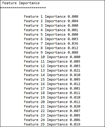
Finally, we can also see the importance associated with each feature:
    print "
 Feature Importance"
    print "======================
"
    for i,score in enumerate(model.feature_importances_):
        print "	Feature %d Importance %0.3f"%(i+1,score)
Let us see how the features are stacked against each other.
Gradient Boosting unifies feature selection and model building into a single operation. It can naturally discover the non-linear relationship between features. Please refer to the following paper on how Gradient boosting can be used for feature selection:
Zhixiang Xu, Gao Huang, Kilian Q. Weinberger, and Alice X. Zheng. 2014. Gradient boosted feature selection. In Proceedings of the 20th ACM SIGKDD international conference on Knowledge discovery and data mining(KDD '14). ACM, New York, NY, USA, 522-531.
Let us apply the dev data to the model and look at its performance:
    # Apply the model on dev set
    predicted_y = model_poly.predict(x_dev_poly)
    print "
 Model Performance in Dev set  (Polynomial features)
"
model_worth(y_dev,predicted_y) 
Finally, we look at the test set performance.

As you can see, our ensemble has performed extremely well in our test set as compared to the dev set.
For more information about Gradient Boosting, please refer to the following paper:
Friedman, J. H. (2001). Greedy function approximation: a gradient boosting machine. Annals of Statistics, pages 1189–1232.
In this receipt we explained gradient boosting with a squared loss function. However Gradient Boosting should be viewed as a framework and not as a method. Any differentiable loss function can be used in this framework. Any learning method and a differentiable loss function can be chosen by users and apply it into the Gradient Boosting framework.
Scikit Learn also provides a Gradient Boosting method for classification, called GradientBosstingClassifier.
http://scikit-learn.org/stable/modules/generated/sklearn.ensemble.GradientBoostingClassifier.html
- Understanding Ensemble, Bagging Method recipe in Chapter 8, Model Selection and Evaluation
- Understanding Ensemble, Boosting Method AdaBoost recipe in Chapter 8, Model Selection and Evaluation
- Predicting real valued numbers using regression recipe in Chapter 7, Machine Learning II
- Variable Selection using LASSO Regression recipe in Chapter 7, Machine Learning II
- Using cross validation iterators recipe in Chatper 7, Machine Learning II