
We will look at a document classification problem in this recipe. The algorithm that we will use is the Naïve Bayes classifier. The Bayes' rule is the engine powering the Naïve Bayes algorithm, as follows:
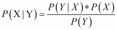
It shows how likely it is for the event X to happen, given that we know event Y has already happened. Now, in our recipe, we will categorize or classify the text. Ours is a binary classification problem: given a movie review, we want to classify if the review is positive or negative.
In Bayesian terminology, we need to find the conditional probability: the probability that the review is positive given the review, and the probability that the review is negative given the review. Let's write it as an equation:
For any review, if we have the preceding two probability values, we can classify the review as positive or negative by comparing these values. If the conditional probability for negative is greater than the conditional probability for positive, we classify the review as negative, and vice versa.
Let's now discuss these probabilities using Bayes' rule:

As we are going to compare these two equations to finalize our prediction, we can ignore the denominator, which is a simple scaling factor.
The LHS (left-hand side) of the preceding equation is called the posterior probability.
Let's look at the numerator of the RHS (right-hand side):
P(positive) is the probability of a positive class called the prior. It's our belief about the positive class label distribution based on our training set.
We will estimate it from our training test. It's calculated as follows:

P(review|positive) is the likelihood. It answers the question: what is the likelihood of getting the review, given that the class is positive. Again, we will estimate it from our training set.
Before we expand on the likelihood equation further, let's introduce the concept of independence assumption. The algorithm is prefixed as naïve because of this assumption. Contrary to the reality, we assume that the words appear in a document independent of each other. We will use this assumption to calculate the likelihood.
A review is a list of words. Let's put it in mathematical notation:
With the independence assumption, we can say that the probability of each of these words occurring together in a review is the product of all the individual probabilities of the constituent words in the review.
Now we can write the likelihood equation as follows:

So, given a new review, we can use these two equations, the prior and likelihood, to calculate whether the review is positive or negative.
Hopefully, you have followed till now. There is still a one last piece to the puzzle: how do we calculate the probability for the individual words?

This step refers to training the model.
From our training set, we will take each review. We also know its label. For each word in this review, we will calculate the conditional probability and store it in a table. We can thus use these values to predict any future test instance.
Enough theory! Let's dive into our recipe.
For this recipe, we will use the NLTK library for both the data and the algorithm. During the installation of NLTK, we can also download the datasets. One such dataset is the movie review dataset. The movie review data is segregated into two categories, positive and negative. For each category, we have a list of words; the reviews are preseparated into words:
from nltk.corpus import movie_reviews
As shown here, we will include the datasets by importing the corpus module from NLTK.
We will leverage the NaiveBayesClassifier class, defined in NLTK, to build the model. We will pass our training data to a function called train() to build our model.
Let's start with importing the necessary function. We will follow it up with two utility functions. The first one retrieves the movie review data and the second one helps us split our data for the model into training and testing:
from nltk.corpus import movie_reviews
from sklearn.cross_validation import StratifiedShuffleSplit
import nltk
from nltk.corpus import stopwords
from nltk.collocations import BigramCollocationFinder
from nltk.metrics import BigramAssocMeasures


def get_data():
    """
    Get movie review data
    """
    dataset = []
    y_labels = []
    # Extract categories
    for cat in movie_reviews.categories():
        # for files in each cateogry
        for fileid in movie_reviews.fileids(cat):
            # Get the words in that category
            words = list(movie_reviews.words(fileid))
            dataset.append((words,cat))
            y_labels.append(cat)
    return dataset,y_labels


def get_train_test(input_dataset,ylabels):
    """
    Perpare a stratified train and test split
    """
    train_size = 0.7
    test_size = 1-train_size
    stratified_split = StratifiedShuffleSplit(ylabels,test_size=test_size,n_iter=1,random_state=77)

    for train_indx,test_indx in stratified_split:
        train   = [input_dataset[i] for i in train_indx]
        train_y = [ylabels[i] for i in train_indx]

        test    = [input_dataset[i] for i in test_indx]
        test_y  = [ylabels[i] for i in test_indx]
    return train,test,train_y,test_y
We will now introduce three functions, which are primarily feature-generating functions. We need to provide features or attributes to our classifier. These functions, given a review, generate a set of features from the review:
def build_word_features(instance):
    """
    Build feature dictionary
    Features are binary, name of the feature is word iteslf
    and value is 1. Features are stored in a dictionary
    called feature_set
    """
    # Dictionary to store the features
    feature_set = {}
    # The first item in instance tuple the word list
    words = instance[0]
    # Populate feature dicitonary
    for word in words:
        feature_set[word] = 1
    # Second item in instance tuple is class label
    return (feature_set,instance[1])

def build_negate_features(instance):
    """
    If a word is preceeded by either 'not' or 'no'
    this function adds a prefix 'Not_' to that word
    It will also not insert the previous negation word
    'not' or 'no' in feature dictionary
    """
    # Retreive words, first item in instance tuple
    words = instance[0]
    final_words = []
    # A boolean variable to track if the
    # previous word is a negation word
    negate = False
    # List of negation words
    negate_words = ['no','not']
    # On looping throught the words, on encountering
    # a negation word, variable negate is set to True
    # negation word is not added to feature dictionary
    # if negate variable is set to true
    # 'Not_' prefix is added to the word
    for word in words:
        if negate:
            word = 'Not_' + word
            negate = False
        if word not in negate_words:
            final_words.append(word)
        else:
            negate = True
    # Feature dictionary
    feature_set = {}
    for word in final_words:
        feature_set[word] = 1
    return (feature_set,instance[1])

def remove_stop_words(in_data):
    """
    Utility function to remove stop words
    from the given list of words
    """
    stopword_list = stopwords.words('english')
    negate_words = ['no','not']
    # We dont want to remove the negate words
    # Hence we create a new stop word list excluding
    # the negate words
    new_stopwords = [word for word in stopword_list if word not in negate_words]
    label = in_data[1]
    # Remove stopw words
    words = [word for word in in_data[0] if word not in new_stopwords]
    return (words,label)


def build_keyphrase_features(instance):
    """
    A function to extract key phrases
    from the given text.
    Key Phrases are words of importance according to a measure
    In this key our phrase of is our length 2, i.e two words or bigrams
    """
    feature_set = {}
    instance = remove_stop_words(instance)
    words = instance[0]

    bigram_finder  = BigramCollocationFinder.from_words(words)
    # We use the raw frequency count of bigrams, i.e. bigrams are
    # ordered by their frequency of occurence in descending order
    # and top 400 bigrams are selected.
    bigrams        = bigram_finder.nbest(BigramAssocMeasures.raw_freq,400)
    for bigram in bigrams:
        feature_set[bigram] = 1
    return (feature_set,instance[1])
Let's now write a function to build our model and later probe our model to find the usefulness of our model:
def build_model(features):
    """
    Build a naive bayes model
    with the gvien feature set.
    """
    model = nltk.NaiveBayesClassifier.train(features)
    return model

def probe_model(model,features,dataset_type = 'Train'):
    """
    A utility function to check the goodness
    of our model.
    """
    accuracy = nltk.classify.accuracy(model,features)
    print "
" + dataset_type + " Accuracy = %0.2f"%(accuracy*100) + "%"

def show_features(model,no_features=5):
    """
    A utility function to see how important
    various features are for our model.
    """
    print "
Feature Importance"
    print "===================
"
    print model.show_most_informative_features(no_features)
It is very hard to get the model right at the first pass. We need to play around with different features, and parameter tuning. This is mostly a trial and error process. In the next section of code, we will show our different passes by improving our model:
def build_model_cycle_1(train_data,dev_data):
    """
    First pass at trying out our model
    """
    # Build features for training set
    train_features =map(build_word_features,train_data)
    # Build features for test set
    dev_features = map(build_word_features,dev_data)
    # Build model
    model = build_model(train_features)
    # Look at the model
    probe_model(model,train_features)
    probe_model(model,dev_features,'Dev')

    return model

def build_model_cycle_2(train_data,dev_data):
    """
    Second pass at trying out our model
    """

    # Build features for training set
    train_features =map(build_negate_features,train_data)
    # Build features for test set
    dev_features = map(build_negate_features,dev_data)
    # Build model
    model = build_model(train_features)
    # Look at the model
    probe_model(model,train_features)
    probe_model(model,dev_features,'Dev')

    return model


def build_model_cycle_3(train_data,dev_data):
    """
    Third pass at trying out our model
    """

    # Build features for training set
    train_features =map(build_keyphrase_features,train_data)
    # Build features for test set
    dev_features = map(build_keyphrase_features,dev_data)
    # Build model
    model = build_model(train_features)
    # Look at the model
    probe_model(model,train_features)
    probe_model(model,dev_features,'Dev')
    test_features = map(build_keyphrase_features,test_data)
    probe_model(model,test_features,'Test')

    return model
Finally, we will write a code with which we can invoke all our functions that were defined previously:
if __name__ == "__main__":

    # Load data
    input_dataset, y_labels = get_data()
    # Train data
    train_data,all_test_data,train_y,all_test_y = get_train_test(input_dataset,y_labels)
    # Dev data
    dev_data,test_data,dev_y,test_y = get_train_test(all_test_data,all_test_y)

    # Let us look at the data size in our different
    # datasets
    print "
Original  Data Size   =", len(input_dataset)
    print "
Training  Data Size   =", len(train_data)
    print "
Dev       Data Size   =", len(dev_data)
    print "
Testing   Data Size   =", len(test_data)

    # Different passes of our model building exercise
    model_cycle_1 =  build_model_cycle_1(train_data,dev_data)
    # Print informative features
    show_features(model_cycle_1)
    model_cycle_2 = build_model_cycle_2(train_data,dev_data)
    show_features(model_cycle_2)
    model_cycle_3 = build_model_cycle_3(train_data,dev_data)
show_features(model_cycle_3)Let's try to follow this recipe from the main function. We started with invoking the get_data function. As explained before, the movie review data is stored as two categories, positive and negative. Our first loop goes through these categories. With these categories, we retrieved the file IDs for these categories in the second loop. Using these file IDs, we retrieve the words, as follows:
words = list(movie_reviews.words(fileid))
We will append these words to a list called dataset. The class label is appended to another list called y_labels.
Finally, we return the words and corresponding class labels:
return dataset,y_labels
Equipped with the dataset, we need to divide this dataset into the test and the train datasets:
 # Train data
    train_data,all_test_data,train_y,all_test_y = get_train_test(input_dataset,y_labels)
We invoked the get_train_test function with an input dataset and the class labels. This function provides us with a stratified sample. We are using 70 percent of our data for the training set and the rest for the test set.
Once again, we invoke get_train_test with the test dataset returned from the previous step:
    # Dev data
    dev_data,test_data,dev_y,test_y = get_train_test(all_test_data,all_test_y)
We created a separate dataset and called it the dev dataset. We need this dataset to tune our model. We want our test set to really behave as a test set. We don't want to expose our test set during the different passes of our model building exercise.
Let's print the size of our train, dev, and test datasets:

As you can see, 70 percent of the original data is assigned to our training set. We have again split the rest 30 percent into a 70/30 percent split for Dev and Testing.
Let's start our model building activity. We will call build_model_cycle_1 with our training and dev datasets. In this function, we will first create our features by calling build_word_feature using a map on all the instances in our dataset. The build_word_feature is a simple feature-generating function. Every word is a feature. The output of this function is a dictionary of features, where the key is the word itself and the value is one. These types of features are typically called Bag of Words (BOW). The build_word_features is invoked using both the training and the dev data:
    # Build features for training set
    train_features =map(build_negate_features,train_data)
    # Build features for test set
    dev_features = map(build_negate_features,dev_data)
We will now proceed to train our model with the generated feature:
    # Build model
    model = build_model(train_features)
We need to test how good our model is. We use the probe_model function to do this. Probe_model takes three parameters. The first parameter is the model of interest, the second parameter is the feature against which we want to see how good our model is, and the last parameter is a string used for display purposes. The probe_model function calculates the accuracy metric using the accuracy function in the nltk.classify module.
We invoke probe_model twice: once with the training data to see how good the model is on our training dataset, and then once with our dev dataset:
    # Look at the model
    probe_model(model,train_features)
    probe_model(model,dev_features,'Dev')
Let's now look at the accuracy figures:

Our model is behaving very well using the training data. This is not surprising as the model has already seen it during the training phase. It's doing a good job at classifying the training record correctly. However, our dev accuracy is very poor. Our model is able to classify only 60 percent of the dev instances correctly. Surely our features are not informative enough to help our model classify the unseen instances with a good accuracy. It will be good to see which features are contributing more towards discriminating a review into positive and negative:
show_features(model_cycle_1)
We will invoke the show_features function to look at the features' contribution towards the model. The Show_features function utilizes the show_most_informative_feature function from the NLTK classifier object. The most important features in our first model are as follows:

The way to read it is: the feature stupidity = 1 is 15 times more effective for classifying a review as negative.
Let's now do a second round of building this model using a new set of features. We will do this by invoking build_model_cycle_2. build_model_cycle_2 is very similar to build_model_cycle_1 except for the feature generation function called inside map function.
The feature generation function is called build_negate_features. Typically, words such as not and no are called negation words. Let's assume that our reviewer says that the movie is not good. If we use our previous feature generator, the word good would be treated equally in both the positive and negative reviews. We know that the word good should be used to discriminate the positive reviews. To avoid this problem, we will look for the negation words no and not in our word list. We want to modify our example sentence as follows:
"movie is not good" to "movie is not_good"
This way, no_good can be used as a good feature to discriminate the negative reviews from the positive reviews. The build_negate_features function does this job.
Let's now look at our probing output for the model built with this negation feature:

We improved our model accuracy on our dev data by almost 2 percent. Let's now look at the most informative features for this model:

Look at the last feature. Adding negation to funny, the 'Not_funny' feature is 11.7 times more informative for discriminating a review as negative.
Can we do better on our model accuracy ? Currently, we are at 70 percent. Let's do a third run with a new set of features. We will do this by invoking build_model_cycle_3. build_model_cycle_3 is very similar to build_model_cycle_2 except for the feature generation function called inside map function.
The build_keyphrase_features function is used as a feature generator. Let's look at the function in detail. Instead of using the words as features, we will generate key phrases from the review and use them as features. Key phrases are phrases that we consider important using some metric. Key phrases can be made of either two, three, or n words. In our case, we will use two words (bigrams) to build our key phrase. The metric that we will use is the raw frequency count of these phrases. We will choose the phrases whose frequency count is higher. We will do some simple preprocessing before generating our key phrases. We will remove all the stopwords and punctuation from our word list. The remove_stop_words function is invoked to remove the stopwords and punctuation. NLTK's corpus module has a list of English stopwords. We can retrieve it as follows:
stopword_list = stopwords.words('english')Similarly, the string module in Python maintains a list of punctuation. We will remove the stopwords and punctuation as follows:
words = [word for word in in_data[0] if word not in new_stopwords
and word not in punctuation]
However, we will not remove not and no. We will create a new set of stopwords by not, including the negation words in the previous step:
new_stopwords = [word for word in stopword_list if word not in negate_words]
We will leverage the BigramCollocationFinder class from NLTK to generate our key phrases:
    bigram_finder  = BigramCollocationFinder.from_words(words)
    # We use the raw frequency count of bigrams, i.e. bigrams are
    # ordered by their frequency of occurence in descending order
    # and top 400 bigrams are selected.
    bigrams        = bigram_finder.nbest(BigramAssocMeasures.raw_freq,400)
Our metric is the frequency count. You can see that we specified it as raw_freq in the last line. We will ask the collocation finder to return us a maximum of 400 phrases.
Loaded with our new feature, we will proceed to build our model and test the correctness of our model. Let's look at the output of our model:
Yes! We have achieved a great deal of improvement on our dev set. From 68 percent accuracy in our first pass with word features, we have moved from 12 percent up to 80 percent with our key phrase features. Let's now expose our test set to this model and check the accuracy:
    test_features = map(build_keyphrase_features,test_data)
    probe_model(model,test_features,'Test')
Our test set's accuracy is greater than our dev set's accuracy. We did a good job in training a good model that works well on an unseen dataset. Before we end this recipe, let's look at the key phrases that are the most informative:

The key phrase, Oscar nomination, is 10 times more helpful in discriminating a review as positive. You can't deny this. We can see that our key phrases are very informative, and hence, our model performed better than the previous two runs.
How did we know that 400 key phrases and the metric frequency count is the best parameter for bigram generation? Trial and error. Though we didn't list our trial and error process, we pretty much ran it with various combinations such as 200 phrases with pointwise mutual information, and similar other methods.
This is what needs to be done in the real world. However, instead of a blind search through the parameter space every time, we looked at the most informative features. This gave us a clue on the discriminating power of the features.
- Preparing data for model building recipe in Chapter 6, Machine Learning I