
Boosting is a powerful ensemble technique. It's pretty much used in most of the Data Science applications. In fact, it is one of the most essential tools in a Data Scientist tool kit. The Boosting technique utilizes a bag of estimators similar to Bagging. But that is where the similarity ends. Let us quickly see how Boosting acts as a very effective ensemble technique before jumping into our recipe.
Let's take the familiar two-class classification problem, where the input is a set of predictors (X) and the output is a response variable (Y) which can either take 0 or 1 as value. The input for the classification problem is represented as follows:
The job the classifier is to find a function which can approximate:
The misclassification rate of the classifier is defined as:

Let us say we build a very weak classifier whose error rate is slightly better than random guessing. In Boosting, we build a sequence of weak classifiers on a slightly modified set of data. We modify the data slightly for every classifier, and finally, we end up with M classifiers:
Finally, the predictions from all of them are combined through a weighted majority vote:

This method is called AdaBoost.
The weight alpha and the sequential way of model building is where Boosting differs from Bagging. As mentioned earlier, Boosting builds a sequence of weak classifiers on a slightly modified data set for each classifier. Let us look at what that slight data modification refers to. It is from this modification that we derive our weight alpha.
Initially for the first classifier, m=1, we set the weight of each instance as 1/N, that is, if there are a hundred records, each record gets a weight of 0.001. Let us denote the weight by w—now we have a hundred such weights:
All the records now have an equal chance of being selected by a classifier. We build the classifier, and test it against our training data to get the misclassification rate. Refer to the misclassification rate formula given earlier in this section. We are going to change it slightly by including the weights, as follows:

Where abs stands for the absolute value of the results. With this error rate, we calculate our alpha (model weight) as follows:

Where epsilon is a very small value.
Let us say our model 1 has got an error rate of 0.3, that is, the model was able to classify 70 percent of the records correctly. Therefore, the weight for that model will be 0.8, approximately, which, is a good weight. Based on this, we go will back and set the weights of individual records, as follows:
As you can see, the weights of all the attributes which were misclassified will increase. This increases the chance of the misclassified record being selected by the next classifier. Thus, the classifier coming next in the sequence selects the instances with more weight and tries to fit it. In this way, all the future classifiers start concentrating on the records misclassified by the previous classifier.
This is the power of boosting. It is able to turn several weak classifiers into one powerful ensemble.
Let us see boosting in action. As we proceed with our code, we will also see a small variation to AdaBoost known as SAMME.
We will leverage the scikit learn classes DecisionTreeClassifier for classification and the AdaBoostClassifier for applying the Boosting principle. We will generate data for this recipe using the make_classification convenience function.
Let us import the necessary libraries, and write a function get_data() to provide us with a dataset to work through this recipe.
from sklearn.datasets import make_classification
from sklearn.ensemble import AdaBoostClassifier
from sklearn.metrics import classification_report,zero_one_loss
from sklearn.cross_validation import train_test_split
from sklearn.tree import DecisionTreeClassifier
import numpy as np
import matplotlib.pyplot as plt
import itertools

def get_data():
    """
    Make a sample classification dataset
    Returns : Independent variable y, dependent variable x
    """
    no_features = 30
    redundant_features = int(0.1*no_features)
    informative_features = int(0.6*no_features)
    repeated_features = int(0.1*no_features)
    print no_features,redundant_features,informative_features,repeated_features
    x,y = make_classification(n_samples=500,n_features=no_features,flip_y=0.03,
            n_informative = informative_features, n_redundant = redundant_features
            ,n_repeated = repeated_features,random_state=7)
    return x,y

def build_single_model(x,y):
    model = DecisionTreeClassifier()
    model.fit(x,y)
    return model

def build_boosting_model(x,y,no_estimators=20):
    boosting = AdaBoostClassifier(DecisionTreeClassifier(max_depth=1,min_samples_leaf=1),random_state=9
    ,n_estimators=no_estimators,algorithm="SAMME")
    boosting.fit(x,y)
    return boosting

def view_model(model):
    print "
 Estimator Weights and Error
"
    for i,weight in  enumerate(model.estimator_weights_):
        print "estimator %d weight = %0.4f error = %0.4f"%(i+1,weight,model.estimator_errors_[i])

    plt.figure(1)
    plt.title("Model weight vs error")
    plt.xlabel("Weight")
    plt.ylabel("Error")
    plt.plot(model.estimator_weights_,model.estimator_errors_)


def number_estimators_vs_err_rate(x,y,x_dev,y_dev):
    no_estimators = range(20,120,10)
    misclassy_rate = []
    misclassy_rate_dev = []

    for no_estimator in no_estimators:
        boosting = build_boosting_model(x,y,no_estimators=no_estimator)
        predicted_y = boosting.predict(x)
        predicted_y_dev = boosting.predict(x_dev)
        misclassy_rate.append(zero_one_loss(y,predicted_y))
        misclassy_rate_dev.append(zero_one_loss(y_dev,predicted_y_dev))

    plt.figure(2)
    plt.title("No estimators vs Mis-classification rate")
    plt.xlabel("No of estimators")
    plt.ylabel("Mis-classification rate")
    plt.plot(no_estimators,misclassy_rate,label='Train')
    plt.plot(no_estimators,misclassy_rate_dev,label='Dev')

    plt.show()


if __name__ == "__main__":
    x,y = get_data()
    plot_data(x,y)

    # Divide the data into Train, dev and test
    x_train,x_test_all,y_train,y_test_all = train_test_split(x,y,test_size = 0.3,random_state=9)
    x_dev,x_test,y_dev,y_test = train_test_split(x_test_all,y_test_all,test_size=0.3,random_state=9)

    # Build a single model
    model = build_single_model(x_train,y_train)
    predicted_y = model.predict(x_train)
    print "
 Single Model Accuracy on training data
"
    print classification_report(y_train,predicted_y)
    print "Fraction of misclassfication = %0.2f"%(zero_one_loss(y_train,predicted_y)*100),"%"


    # Build a bag of models
    boosting = build_boosting_model(x_train,y_train, no_estimators=85)
    predicted_y = boosting.predict(x_train)
    print "
 Boosting Model Accuracy on training data
"
    print classification_report(y_train,predicted_y)
    print "Fraction of misclassfication = %0.2f"%(zero_one_loss(y_train,predicted_y)*100),"%"

    view_model(boosting)

    # Look at the dev set
    predicted_y = model.predict(x_dev)
    print "
 Single Model Accuracy on Dev data
"
    print classification_report(y_dev,predicted_y)
    print "Fraction of misclassfication = %0.2f"%(zero_one_loss(y_dev,predicted_y)*100),"%"

    print "
 Boosting Model Accuracy on Dev data
"
    predicted_y = boosting.predict(x_dev)
    print classification_report(y_dev,predicted_y)
    print "Fraction of misclassfication = %0.2f"%(zero_one_loss(y_dev,predicted_y)*100),"%"

    number_estimators_vs_err_rate(x_train,y_train,x_dev,y_dev)
Let us proceed and write the following three functions:
The function build_single_model to make a simple Decision Tree model with the given data.
The function build_boosting_model, a function which implements the Boosting routine.
The function view_model, to inspect the model that we have built.
def build_single_model(x,y):
    model = DecisionTreeClassifier()
    model.fit(x,y)
    return model

def build_boosting_model(x,y,no_estimators=20):
    boosting = AdaBoostClassifier(DecisionTreeClassifier(max_depth=1,min_samples_leaf=1),random_state=9
    ,n_estimators=no_estimators,algorithm="SAMME")
    boosting.fit(x,y)
    return boosting

def view_model(model):
    print "
 Estimator Weights and Error
"
    for i,weight in  enumerate(model.estimator_weights_):
        print "estimator %d weight = %0.4f error = %0.4f"%(i+1,weight,model.estimator_errors_[i])

    plt.figure(1)
    plt.title("Model weight vs error")
    plt.xlabel("Weight")
    plt.ylabel("Error")
    plt.plot(model.estimator_weights_,model.estimator_errors_)
We then write a function called number_estimators_vs_err_rate. We use this function to see how our error rates change with respect to the number of models in our ensemble.
def number_estimators_vs_err_rate(x,y,x_dev,y_dev):
    no_estimators = range(20,120,10)
    misclassy_rate = []
    misclassy_rate_dev = []

    for no_estimator in no_estimators:
        boosting = build_boosting_model(x,y,no_estimators=no_estimator)
        predicted_y = boosting.predict(x)
        predicted_y_dev = boosting.predict(x_dev)
        misclassy_rate.append(zero_one_loss(y,predicted_y))
        misclassy_rate_dev.append(zero_one_loss(y_dev,predicted_y_dev))

    plt.figure(2)
    plt.title("No estimators vs Mis-classification rate")
    plt.xlabel("No of estimators")
    plt.ylabel("Mis-classification rate")
    plt.plot(no_estimators,misclassy_rate,label='Train')
    plt.plot(no_estimators,misclassy_rate_dev,label='Dev')

    plt.show()
Finally, we will write our main function, which will call the other functions.
if __name__ == "__main__":
    x,y = get_data()
    plot_data(x,y)

    # Divide the data into Train, dev and test
    x_train,x_test_all,y_train,y_test_all = train_test_split(x,y,test_size = 0.3,random_state=9)
    x_dev,x_test,y_dev,y_test = train_test_split(x_test_all,y_test_all,test_size=0.3,random_state=9)

    # Build a single model
    model = build_single_model(x_train,y_train)
    predicted_y = model.predict(x_train)
    print "
 Single Model Accuracy on training data
"
    print classification_report(y_train,predicted_y)
    print "Fraction of misclassfication = %0.2f"%(zero_one_loss(y_train,predicted_y)*100),"%"


    # Build a bag of models
    boosting = build_boosting_model(x_train,y_train, no_estimators=85)
    predicted_y = boosting.predict(x_train)
    print "
 Boosting Model Accuracy on training data
"
    print classification_report(y_train,predicted_y)
    print "Fraction of misclassfication = %0.2f"%(zero_one_loss(y_train,predicted_y)*100),"%"

    view_model(boosting)

    # Look at the dev set
    predicted_y = model.predict(x_dev)
    print "
 Single Model Accuracy on Dev data
"
    print classification_report(y_dev,predicted_y)
    print "Fraction of misclassfication = %0.2f"%(zero_one_loss(y_dev,predicted_y)*100),"%"

    print "
 Boosting Model Accuracy on Dev data
"
    predicted_y = boosting.predict(x_dev)
    print classification_report(y_dev,predicted_y)
    print "Fraction of misclassfication = %0.2f"%(zero_one_loss(y_dev,predicted_y)*100),"%"

number_estimators_vs_err_rate(x_train,y_train,x_dev,y_dev)Let us start with the main method. We first call the get_data function to return the dataset as a matrix x of predictors and a vector y for the response variable. Let us look into the get_data function:
    no_features = 30
    redundant_features = int(0.1*no_features)
    informative_features = int(0.6*no_features)
    repeated_features = int(0.1*no_features)
 x,y =make_classification(n_samples=500,n_features=no_features,flip_y=0.03,
n_informative = informative_features, n_redundant = redundant_features
            ,n_repeated = repeated_features,random_state=7)
Take a look at the parameters passed to the make_classification method. The first parameter is the number of instances required; in this case, we say we need 500 instances. The second parameter gives the number of attributes that are required per instance. We say that we need 30 of them, as defined by the variable no_features. The third parameter flip_y, randomly interchanges 3 percent of the instances. This is done to introduce some noise in our data. The next parameter specifies the number of features out of those 30 which should be informative enough to be used in our classification. We have specified that 60 percent of our features, that is, 18 out of 30 should be informative. The next parameter is about redundant features. These are generated as a linear combination of the informative features for introducing a correlation among the features. Finally, repeated features are the duplicate features which are drawn randomly from both, informative features and redundant features.
Let us split the data into a training and a testing set using train_test_split. We reserve 30 percent of our data for testing.
    # Divide the data into Train, dev and test
    x_train,x_test_all,y_train,y_test_all = train_test_split(x,y,test_size = 0.3,random_state=9)
Once again, we leverage train_test_split to split our test data into dev and test.
x_dev,x_test,y_dev,y_test = train_test_split(x_test_all,y_test_all,test_size=0.3,random_state=9)
Having divided the data for building, evaluating, and testing the model, we proceed to build our models.
Let us start by fitting a single decision tree, and look at the performance of the tree on training set:
    # Build a single model
    model = build_single_model(x_train,y_train)
We build a model by invoking build_single_model function with the predictors and response variable. Inside this we fit a single decision tree and return the tree back to the calling function.
def build_single_model(x,y):
    model = DecisionTreeClassifier()
    model.fit(x,y)
    return model
Let us evaluate how good the model is using classification_report, a utility function from Scikit learn which displays a set of metrics including precision, recall and f1-score; we also display the misclassification rate.
    predicted_y = model.predict(x_train)
    print "
 Single Model Accuracy on training data
"
    print classification_report(y_train,predicted_y)
    print "Fraction of misclassfication =
           %0.2f"%(zero_one_loss(y_train,predicted_y)*100),"%"
As you can see, our decision tree model has done a perfect job of fitting the data—our misclassification rate is 0. Before we test this model on our dev data, let us build our ensemble:
    # Build a bag of models
    boosting = build_boosting_model(x_train,y_train, no_estimators=85)
Using the method build_boosting_model, we build our ensemble as follows:
    boosting = AdaBoostClassifier(DecisionTreeClassifier(max_depth=1,min_samples_leaf=1),random_state=9
    ,n_estimators=no_estimators,algorithm="SAMME")
    boosting.fit(x,y)
We leverage AdaBoostClassifier from Scikit learn to build our Boosting ensemble. We instantiate the class with the following parameters:
An estimator—in our case, we say we want to build an ensemble of decision trees. Hence, we pass the DecisionTreeClassifier object.
max_depth—We don't want to have fully grown trees in our ensemble. We need only stumps—trees with just two leaf nodes and one splitting node. Hence, we set the max_depth parameter to 1.
With the n_estimators parameters, we specify the number of trees that we want to grow; in this case, we will grow 86 trees.
Finally, we have a parameter called algorithm, which is set to SAMME. SAMME stands for Stage wise Additive Modeling using Multi-class Exponential loss function. SAMME is an improvement over the AdaBoosting algorithm. It tries to put more weights on the misclassified records. The model weight alpha is where SAMME differs from AdaBoost.

We have ignored the constant 0.5 in the preceding formula. Let us look at the new addition: log (K-1). If K = 2, then the preceding equation reduces to AdaBoost. Here, K is the number of classes in our response variable. For a two-class problem, SAMME reduces to AdaBoost, as stated earlier.
Let us fit the model, and return it to our calling function. We run this model on our training dataset, and once again look at how the model has performed:
    predicted_y = boosting.predict(x_train)
    print "
 Boosting Model Accuracy on training data
"
    print classification_report(y_train,predicted_y)
    print "Fraction of misclassfication = %0.2f"%(zero_one_loss(y_train,predicted_y)*100),"%"
The result is not very different from our original model. We have correctly classified almost 98 percent of the records with this ensemble.
Before testing it on our dev set, let us proceed to look at the Boosting ensemble that we have built:
view_model(boosting)
Inside view_model, we first print out the weights assigned to each classifier in our ensemble:
    print "
 Estimator Weights and Error
"
    for i,weight in  enumerate(model.estimator_weights_):
        print "estimator %d weight = %0.4f error = %0.4f"%(i+1,weight,model.estimator_errors_[i])
Here we have shown the weights of the first 20 ensembles. Based on their misclassification rate, we have assigned different weights to these estimators.
Let us proceed to plot a graph showing the estimator weight versus the error thrown by each estimator:
    plt.figure(1)
    plt.title("Model weight vs error")
    plt.xlabel("Weight")
    plt.ylabel("Error")
    plt.plot(model.estimator_weights_,model.estimator_errors_)
As you can see, the models which are classifying properly are assigned more weights than the ones with higher errors.
Let us now look at the way single tree and the bag of tree have performed against the dev data:
    # Look at the dev set
    predicted_y = model.predict(x_dev)
    print "
 Single Model Accuracy on Dev data
"
    print classification_report(y_dev,predicted_y)
    print "Fraction of misclassfication = %0.2f"%(zero_one_loss(y_dev,predicted_y)*100),"%"

    print "
 Boosting Model Accuracy on Dev data
"
    predicted_y = boosting.predict(x_dev)
    print classification_report(y_dev,predicted_y)
    print "Fraction of misclassfication = %0.2f"%(zero_one_loss(y_dev,predicted_y)*100),"%"
Pretty much as we did with the training data, we print the classification report and the misclassification rate:

As you can see, the single tree has performed poorly. Though it displayed a 100 percent accuracy with the training data, with the dev data it has misclassified almost 40 percent of the records—a sign of overfitting. In contrast, the Boosting model is able to make a better fit of the dev data.
How do we go about improving the Boosting model? One way to do it is to test the error rate in the training set against the number of ensembles that we want to include in our bagging.
number_estimators_vs_err_rate(x_train,y_train,x_dev,y_dev)
The following function proceeds to fit with the increasing number of ensembles and plot the error rate:
def number_estimators_vs_err_rate(x,y,x_dev,y_dev):
    no_estimators = range(20,120,10)
    misclassy_rate = []
    misclassy_rate_dev = []

    for no_estimator in no_estimators:
        boosting = build_boosting_model(x,y,no_estimators=no_estimator)
        predicted_y = boosting.predict(x)
        predicted_y_dev = boosting.predict(x_dev)
        misclassy_rate.append(zero_one_loss(y,predicted_y))
        misclassy_rate_dev.append(zero_one_loss(y_dev,predicted_y_dev))

    plt.figure(2)
    plt.title("No estimators vs Mis-classification rate")
    plt.xlabel("No of estimators")
    plt.ylabel("Mis-classification rate")
    plt.plot(no_estimators,misclassy_rate,label='Train')
    plt.plot(no_estimators,misclassy_rate_dev,label='Dev')

    plt.show()
As you can see, we declare a list, starting with 20 and ending with 120 in step size of 10s. Inside the for loop, we pass each element of this list as the number of estimator parameter to build_boosting_model, and then proceed to access the error rate of the model. We then check the error rates in the dev set. Now we have two lists—one which has all the error rates from the training data and another with the error rates from the dev data. We plot them both, where the x axis is the number of estimators and y axis is the misclassification rate in the dev and train sets.
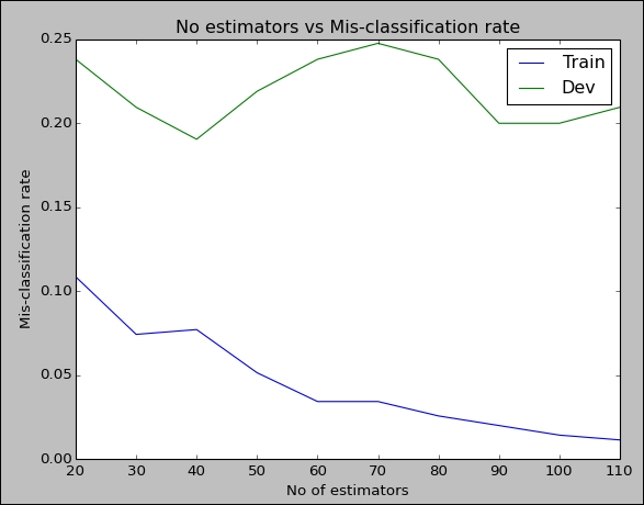
The preceding plot gives a clue that in around 30 to 40 estimators, the error rate in dev is very low. We can further experiment with the tree model parameters to arrive at a good model.
Boosting was introduced in the following seminal paper:
Freund, Y. & Schapire, R. (1997), 'A decision theoretic generalization of on-line learning and an application to boosting', Journal of Computer and System Sciences 55(1), 119–139.
Initially, most of the Boosting methods reduced the multiclass problems into two-class problems and multiple two-class problems. The following paper extends AdaBoost to the multiclass problems:
Multi-class AdaBoost Statistics and Its Interface, Vol. 2, No. 3. (2009), pp. 349-360,doi:10.4310/sii.2009.v2.n3.a8 by Trevor Hastie, Saharon Rosset, Ji Zhu, Hui Zou
This paper also introduces SAMME, the method that we have used in our recipe.