We will use the Iris dataset to demonstrate how to build decision trees. Decision trees are a non-parametric supervised learning method that can be used to solve both classification and regression problems. As explained previously, the advantages of using decision trees are manifold, as follows:

Decision trees are not without problems. Some of the problems that they pose are as follows:

An important part of decision trees is the feature test condition. Let's spend some time understanding the feature test condition. Typically, each attribute in our instance can be either understood.

Binary attribute: This is where an attribute can take two possible values, for example, true or false. The feature test condition should return two values in this case.

Nominal attribute: This is where an attribute can take more than two values, for example, n values. The feature test condition should either output n output or group them into binary splits.

Ordinal attribute: This is where an implicit order in their values exists. For example, let's take an imaginary attribute called size, which can take on the values small, medium, or large. There are three values that the attribute can take and there is an order for them: small, medium, large. They are handled by the feature attribute test condition that is similar to the nominal attribute.

Continuous attributes: These are attributes that can take continuous values. They are discretized into ordinal attributes and then handled.

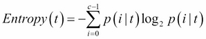
A feature test condition is a way to split the input records into subsets based on a criteria or metric called impurity. This impurity is calculated with respect to the class label for each attribute in the instance. The attribute contributing to the highest impurity is chosen as the data splitting attribute, or in other words, the node for that level in the tree.

Let's see an example to explain it. We will use a measure called entropy to calculate the impurity.

Entropy is defined as follows:

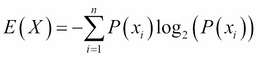
Where:

Let's consider an example:

X = {2,2}

We can now calculate the entropy for this set, as follows:

The entropy for this set is 0. An entropy of 0 indicates homogeneity. It is very easy to code entropy in Python. Look at the following code list:

import math

def prob(data,element):
    """Calculates the percentage count of a given element

    Given a list and an element, returns the elements percentage count
        
    """
    element_count =0
   	# Test conditoin to check if we have proper input
    if len(data) == 0 or element == None 
                or not isinstance(element,(int,long,float)):
        return None      
    element_count = data.count(element)
    return element_count / (1.0 * len(data))


def entropy(data):
    """"Calcuate entropy
    """
    entropy =0.0
    
    if len(data) == 0:
        return None
    
    if len(data) == 1:
        return 0
    try:
        for element in data:
            p = prob(data,element)
            entropy+=-1*p*math.log(p,2)
    except ValueError as e:
        print e.message
        
    
    return entropy

For the purpose of finding the best splitting variable, we will leverage the entropy. First, we will calculate the entropy based on the class labels, as follows:

Let's define another term called information gain. Information gain is a measure to find which attribute in the given instance is most useful for discrimination between the class labels.

Information gain is the difference between an entropy of the parent and an average entropy of the child nodes. At each level in the tree, we will use information gain to build the tree:

https://en.wikipedia.org/wiki/Information_gain_in_decision_trees

We will start with all the attributes in a training set and calculate the overall entropy. Let's look at the following example:

The preceding dataset is imaginary data collected for a user to figure out what kind of movies he is interested in. There are four attributes: the first one is about whether the user watches a movie based on the lead actor, the second attribute is about if the user makes his decision to watch the movie based on whether or not it won an Oscar, and the third one is about if the user decides to watch a movies based on whether or not it is a box office success.

In order to build a decision tree for the preceding example, we will start with the entropy calculation of the whole dataset. This is a two-class problem, hence c = 2. Additionally, there are a total of four records, hence, the entropy of the whole dataset is as follows:

The overall entropy of the dataset is 0.811.

Now, let's look at the first attribute, the lead attribute. For a lead actor, Y, there is one instance class label that says Y and another one that says N. For a lead actor, N, both the instance class labels are N. We will calculate the average entropy as follows:

It's an average entropy. There are two records with a lead actor as Y and two records with lead actors as N; hence, we have 2/4.0 multiplied to the entropy value.

As the entropy is calculated for this subset of data, we can see that out of the two records, one of them has a class label of Y and another one has a class label of N for the lead actor Y. Similarly, for the lead actor N, both the records have a class label of N. Thus, we get the average entropy for this attribute.

The average entropy value for the lead actor attribute is 0.5.

The information gain is now 0.811 – 0.5 = 0.311.

Similarly, we will find the information gain for all the attributes. The attribute with the highest information gain wins and becomes the root node of the decision tree.

The same process is repeated in order to find the second level of the nodes, and so on.

Let's load the required libraries. We will follow it with two functions, one to load the data and the second one to split the data into a training set and a test it:

from sklearn.datasets import load_iris
from sklearn.cross_validation import StratifiedShuffleSplit
import numpy as np
from sklearn import tree
from sklearn.metrics import accuracy_score,classification_report,confusion_matrix
import pprint

def get_data():
    """
    Get Iris data
    """
    data = load_iris()
    x = data['data']
    y = data['target']
    label_names = data['target_names']
    
    return x,y,label_names.tolist()
    

def get_train_test(x,y):
    """
    Perpare a stratified train and test split
    """
    train_size = 0.8
    test_size = 1-train_size
    input_dataset = np.column_stack([x,y])
    stratified_split = StratifiedShuffleSplit(input_dataset[:,-1], 
            test_size=test_size,n_iter=1,random_state = 77)

    for train_indx,test_indx in stratified_split:
        train_x = input_dataset[train_indx,:-1]
        train_y = input_dataset[train_indx,-1]
        test_x =  input_dataset[test_indx,:-1]
        test_y = input_dataset[test_indx,-1]
    return train_x,train_y,test_x,test_y

Let's write the functions to help us build and test the decision tree model:

def build_model(x,y):
    """
    Fit the model for the given attribute 
    class label pairs
    """
    model = tree.DecisionTreeClassifier(criterion="entropy")
    model = model.fit(x,y)
    return model


def test_model(x,y,model,label_names):
    """
    Inspect the model for accuracy
    """
    y_predicted = model.predict(x)
    print "Model accuracy = %0.2f"%(accuracy_score(y,y_predicted) * 100) + "%
"
    print "
Confusion Matrix"
    print "================="
    print pprint.pprint(confusion_matrix(y,y_predicted))
    
    print "
Classification Report"
    print "================="
    
    print classification_report(y,y_predicted,target_names=label_names)

Finally, the main function to invoke all the other functions that we defined is as follows:

if __name__ == "__main__":
    # Load the data
    x,y,label_names = get_data()
    # Split the data into train and test    
    train_x,train_y,test_x,test_y = get_train_test(x,y)
    # Build model    
    model = build_model(train_x,train_y)
    # Evaluate the model on train dataset    
    test_model(train_x,train_y,model,label_names)    
    # Evaluate the model on test dataset
    test_model(test_x,test_y,model,label_names)

Let's start with the main function. We invoke get_data in the x, y, and label_names variables in order to retrieve the Iris dataset. We took the label names so that when we see our model accuracy, we can measure it by individual labels. As said previously, the Iris data poses a three-class problem. We will need to build a classifier that can classify any new instances in one of the tree types: setosa, versicolor, or virginica.

Once again, as in the previous recipes, get_train_test returns stratified train and test datasets. We then leverage StratifiedShuffleSplit from scikit-learn to get the training and test datasets with an equal class label distribution.

We must invoke the build_model method to induce a decision tree on our training set. The DecisionTreeClassifier class in the model tree of scikit-learn implements a decision tree:

model = tree.DecisionTreeClassifier(criterion="entropy")

As you can see, we specified that our feature test condition is an entropy using the criterion variable. We then build the model by calling the fit function and return the model to the calling program.

Now, let's proceed to evaluate our model by using the test_model function. The model takes instances x , class labels y, decision tree model model, and the name of the class labels label_names.

The module metric in scikit-learn provides three evaluation criteria:

from sklearn.metrics import accuracy_score,classification_report,confusion_matrix

We defined accuracy in the previous recipe and the introduction section.

A confusion matrix prints the confusion matrix defined in the introduction section. A confusion matrix is a good way of evaluating the model performance. We are interested in the cell values having true positive and false positive values.

Finally, we also have classification_report to print the precision, recall, and F1 score.

We must evaluate the model on the training data first:

We have done a great job with the training dataset. We have 100 percent accuracy. The true test is with the test dataset where the rubber meets the road.

Let's look at the model evaluation using the test dataset:

Our classifier has performed extremely well with the test set as well.

Let's probe the model to see how the various features contributed towards discriminating the classes.

def get_feature_names():
    data = load_iris()
    return data['feature_names']


def probe_model(x,y,model,label_names):

    feature_names = get_feature_names()
    feature_importance = model.feature_importances_
    print "
Feature Importance
"
    print "=====================
"
    for i,feature_name in enumerate(feature_names):
        print "%s = %0.3f"%(feature_name,feature_importance[i])

    # Export the decison tree as a graph
    tree.export_graphviz(model,out_file='tree.dot')

The tree classifier object provides an attribute called feature_importances_, which can be called to retrieve the importance of the various features towards building our model.

We wrote a simple function, get_feature_names, in order to retrieve the names of our attributes. However, this can be added as a part of get_data.

Let's look at the print statement output:

This looks as if the petal width and petal length are contributing more towards our classification.

Interestingly, we can also export the tree built by the classifier as a dot file and it can be visualized using the GraphViz package. In the last line, we export our model as a dot file:

# Export the decison tree as a graph
tree.export_graphviz(model,out_file='tree.dot')

You can download and install the Graphviz package to visualize this:

http://www.graphviz.org/