Chapter 2. Creating a dataset

 

 

The first step in any data analysis is the creation of a dataset containing the information to be studied, in a format that meets your needs. In R, this task involves the following:

• Selecting a data structure to hold your data
• Entering or importing your data into the data structure

The first part of this chapter (sections 2.1–2.2) describes the wealth of structures that R can use for holding data. In particular, section 2.2 describes vectors, factors, matrices, data frames, and lists. Familiarizing yourself with these structures (and the notation used to access elements within them) will help you tremendously in understanding how R works. You might want to take your time working through this section.

The second part of this chapter (section 2.3) covers the many methods available for importing data into R. Data can be entered manually, or imported from an external source. These data sources can include text files, spreadsheets, statistical packages, and database management systems. For example, the data that I work with typically comes from SQL databases. On occasion, though, I receive data from legacy DOS systems, and from current SAS and SPSS databases. It’s likely that you’ll only have to use one or two of the methods described in this section, so feel free to choose those that fit your situation.

Once a dataset is created, you’ll typically annotate it, adding descriptive labels for variables and variable codes. The third portion of this chapter (section 2.4) looks at annotating datasets and reviews some useful functions for working with datasets (section 2.5). Let’s start with the basics.

2.1. Understanding datasets

A dataset is usually a rectangular array of data with rows representing observations and columns representing variables. Table 2.1 provides an example of a hypothetical patient dataset.

Table 2.1. A patient dataset

PatientID	AdmDate	Age	Diabetes	Status
1	10/15/2009	25	Type1	Poor
2	11/01/2009	34	Type2	Improved
3	10/21/2009	28	Type1	Excellent
4	10/28/2009	52	Type1	Poor

Different traditions have different names for the rows and columns of a dataset. Statisticians refer to them as observations and variables, database analysts call them records and fields, and those from the data mining/machine learning disciplines call them examples and attributes. We’ll use the terms observations and variables throughout this book.

You can distinguish between the structure of the dataset (in this case a rectangular array) and the contents or data types included. In the dataset shown in table 2.1, PatientID is a row or case identifier, AdmDate is a date variable, Age is a continuous variable, Diabetes is a nominal variable, and Status is an ordinal variable.

R contains a wide variety of structures for holding data, including scalars, vectors, arrays, data frames, and lists. Table 2.1 corresponds to a data frame in R. This diversity of structures provides the R language with a great deal of flexibility in dealing with data.

The data types or modes that R can handle include numeric, character, logical (TRUE/FALSE), complex (imaginary numbers), and raw (bytes). In R, PatientID, AdmDate, and Age would be numeric variables, whereas Diabetes and Status would be character variables. Additionally, you’ll need to tell R that PatientID is a case identifier, that AdmDate contains dates, and that Diabetes and Status are nominal and ordinal variables, respectively. R refers to case identifiers as rownames and categorical variables (nominal, ordinal) as factors. We’ll cover each of these in the next section. You’ll learn about dates in chapter 3.

2.2. Data structures

R has a wide variety of objects for holding data, including scalars, vectors, matrices, arrays, data frames, and lists. They differ in terms of the type of data they can hold, how they’re created, their structural complexity, and the notation used to identify and access individual elements. Figure 2.1 shows a diagram of these data structures.

Figure 2.1. R data structures

Let’s look at each structure in turn, starting with vectors.

 

 

2.2.1. Vectors

Vectors are one-dimensional arrays that can hold numeric data, character data, or logical data. The combine function c() is used to form the vector. Here are examples of each type of vector:

a <- c(1, 2, 5, 3, 6, -2, 4)
b <- c("one", "two", "three")
c <- c(TRUE, TRUE, TRUE, FALSE, TRUE, FALSE)

Here, a is numeric vector, b is a character vector, and c is a logical vector. Note that the data in a vector must only be one type or mode (numeric, character, or logical). You can’t mix modes in the same vector.

 

Note

Scalars are one-element vectors. Examples include f <- 3, g <- "US" and h <- TRUE. They’re used to hold constants.

 

You can refer to elements of a vector using a numeric vector of positions within brackets. For example, a[c(2, 4)] refers to the 2nd and 4th element of vector a. Here are additional examples:

> a <- c(1, 2, 5, 3, 6, -2, 4)
> a[3]
[1] 5
> a[c(1, 3, 5)]
[1] 1 5 6
> a[2:6]
[1]  2  5  3  6 -2

The colon operator used in the last statement is used to generate a sequence of numbers. For example, a <- c(2:6) is equivalent to a <- c(2, 3, 4, 5, 6).

2.2.2. Matrices

A matrix is a two-dimensional array where each element has the same mode (numeric, character, or logical). Matrices are created with the matrix function. The general format is

myymatrix <- matrix(vector, nrow=number_of_rows, ncol=number_of_columns,
                    byrow=logical_value, dimnames=list(
                    char_vector_rownames, char_vector_colnames))

where vector contains the elements for the matrix, nrow and ncol specify the row and column dimensions, and dimnames contains optional row and column labels stored in character vectors. The option byrow indicates whether the matrix should be filled in by row (byrow=TRUE) or by column (byrow=FALSE). The default is by column. The following listing demonstrates the matrix function.

Listing 2.1. Creating matrices

First, you create a 5×4 matrix . Then you create a 2×2 matrix with labels and fill the matrix by rows . Finally, you create a 2×2 matrix and fill the matrix by columns .

You can identify rows, columns, or elements of a matrix by using subscripts and brackets. X[i,] refers to the ith row of matrix X, X[, j] refers to jth column, and X[i, j] refers to the ijth element, respectively. The subscripts i and j can be numeric vectors in order to select multiple rows or columns, as shown in the following listing.

Listing 2.2. Using matrix subscripts

> x <- matrix(1:10, nrow=2)
> x
      [,1] [,2] [,3] [,4] [,5]
[1,]     1    3    5    7    9
[2,]    2    4    6    8    10
> x[2,]
  [1]  2  4  6  8 10
> x[,2]
[1] 3 4
> x[1,4]
[1] 7
> x[1, c(4,5)]
[1] 7 9

First a 2 × 5 matrix is created containing numbers 1 to 10. By default, the matrix is filled by column. Then the elements in the 2nd row are selected, followed by the elements in the 2nd column. Next, the element in the 1st row and 4th column is selected. Finally, the elements in the 1st row and the 4th and 5th columns are selected.

Matrices are two-dimensional and, like vectors, can contain only one data type. When there are more than two dimensions, you’ll use arrays (section 2.2.3). When there are multiple modes of data, you’ll use data frames (section 2.2.4).

2.2.3. Arrays

Arrays are similar to matrices but can have more than two dimensions. They’re created with an array function of the following form:

myarray <- array(vector, dimensions, dimnames)

where vector contains the data for the array, dimensions is a numeric vector giving the maximal index for each dimension, and dimnames is an optional list of dimension labels. The following listing gives an example of creating a three-dimensional (2×3×4) array of numbers.

Listing 2.3. Creating an array

> dim1 <- c("A1", "A2")
> dim2 <- c("B1", "B2", "B3")
> dim3 <- c("C1", "C2", "C3", "C4")
> z <- array(1:24, c(2, 3, 4), dimnames=list(dim1, dim2, dim3))
> z
, , C1

   B1 B2 B3
A1  1  3  5
A2  2  4  6


, , C2

   B1 B2 B3
A1  7  9 11
A2  8 10 12


, , C3

   B1 B2 B3
A1 13 15 17
A2 14 16 18


, , C4

   B1 B2 B3
A1 19 21 23
A2 20 22 24

As you can see, arrays are a natural extension of matrices. They can be useful in programming new statistical methods. Like matrices, they must be a single mode. Identifying elements follows what you’ve seen for matrices. In the previous example, the z[1,2,3] element is 15.

2.2.4. Data frames

A data frame is more general than a matrix in that different columns can contain different modes of data (numeric, character, etc.). It’s similar to the datasets you’d typically see in SAS, SPSS, and Stata. Data frames are the most common data structure you’ll deal with in R.

The patient dataset in table 2.1 consists of numeric and character data. Because there are multiple modes of data, you can’t contain this data in a matrix. In this case, a data frame would be the structure of choice.

A data frame is created with the data.frame() function:

mydata <- data.frame(col1, col2, col3,...)

where col1, col2, col3, ... are column vectors of any type (such as character, numeric, or logical). Names for each column can be provided with the names function. The following listing makes this clear.

Listing 2.4. Creating a data frame

> patientID <- c(1, 2, 3, 4)
> age <- c(25, 34, 28, 52)
> diabetes <- c("Type1", "Type2", "Type1", "Type1")
> status <- c("Poor", "Improved", "Excellent", "Poor")
> patientdata <- data.frame(patientID, age, diabetes, status)
> patientdata
  patientID age  diabetes     status
1         1  25     Type1       Poor
2         2  34     Type2   Improved
3         3  28     Type1  Excellent
4         4  52     Type1       Poor

Each column must have only one mode, but you can put columns of different modes together to form the data frame. Because data frames are close to what analysts typically think of as datasets, we’ll use the terms columns and variables interchangeably when discussing data frames.

There are several ways to identify the elements of a data frame. You can use the subscript notation you used before (for example, with matrices) or you can specify column names. Using the patientdata data frame created earlier, the following listing demonstrates these approaches.

Listing 2.5. Specifying elements of a data frame

The $ notation in the third example is new . It’s used to indicate a particular variable from a given data frame. For example, if you want to cross tabulate diabetes type by status, you could use the following code:

> table(patientdata$diabetes, patientdata$status)

        Excellent Improved Poor
  Type1         1        0     2
  Type2         0        1     0

It can get tiresome typing patientdata$ at the beginning of every variable name, so shortcuts are available. You can use either the attach() and detach() or with() functions to simplify your code.

Attach, Detach, and With

The attach() function adds the data frame to the R search path. When a variable name is encountered, data frames in the search path are checked in order to locate the variable. Using the mtcars data frame from chapter 1 as an example, you could use the following code to obtain summary statistics for automobile mileage (mpg), and plot this variable against engine displacement (disp), and weight (wt):

summary(mtcars$mpg)
plot(mtcars$mpg, mtcars$disp)
plot(mtcars$mpg, mtcars$wt)

This could also be written as

attach(mtcars)
  summary(mpg)
  plot(mpg, disp)
  plot(mpg, wt)
detach(mtcars)

The detach() function removes the data frame from the search path. Note that detach() does nothing to the data frame itself. The statement is optional but is good programming practice and should be included routinely. (I’ll sometimes ignore this sage advice in later chapters in order to keep code fragments simple and short.)

The limitations with this approach are evident when more than one object can have the same name. Consider the following code:

> mpg <- c(25, 36, 47)
> attach(mtcars)


The following object(s) are masked _by_ '.GlobalEnv':    mpg
> plot(mpg, wt)
Error in xy.coords(x, y, xlabel, ylabel, log) :
  'x' and 'y' lengths differ
> mpg
[1] 25 36 47

Here we already have an object named mpg in our environment when the mtcars data frame is attached. In such cases, the original object takes precedence, which isn’t what you want. The plot statement fails because mpg has 3 elements and disp has 32 elements. The attach() and detach() functions are best used when you’re analyzing a single data frame and you’re unlikely to have multiple objects with the same name. In any case, be vigilant for warnings that say that objects are being masked.

An alternative approach is to use the with() function. You could write the previous example as

with(mtcars, {
  summary(mpg, disp, wt)
  plot(mpg, disp)
  plot(mpg, wt)
})

In this case, the statements within the {} brackets are evaluated with reference to the mtcars data frame. You don’t have to worry about name conflicts here. If there’s only one statement (for example, summary(mpg)), the {} brackets are optional.

The limitation of the with() function is that assignments will only exist within the function brackets. Consider the following:

> with(mtcars, {
   stats <- summary(mpg)
   stats
  })
   Min. 1st Qu.  Median    Mean 3rd Qu.     Max.
  10.40   15.43   19.20   20.09   22.80    33.90
> stats
Error: object 'stats' not found

If you need to create objects that will exist outside of the with() construct, use the special assignment operator <<- instead of the standard one (<-). It will save the object to the global environment outside of the with() call. This can be demonstrated with the following code:

> with(mtcars, {
   nokeepstats <- summary(mpg)
   keepstats <<- summary(mpg)
})
> nokeepstats
Error: object 'nokeepstats' not found
> keepstats
   Min. 1st Qu.  Median    Mean 3rd Qu.    Max.
    10.40   15.43   19.20   20.09   22.80   33.90

Most books on R recommend using with() over attach(). I think that ultimately the choice is a matter of preference and should be based on what you’re trying to achieve and your understanding of the implications. We’ll use both in this book.

Case Identifiers

In the patient data example, patientID is used to identify individuals in the dataset. In R, case identifiers can be specified with a rowname option in the data frame function. For example, the statement

patientdata <- data.frame(patientID, age, diabetes, status,
  row.names=patientID)

specifies patientID as the variable to use in labeling cases on various printouts and graphs produced by R.

2.2.5. Factors

As you’ve seen, variables can be described as nominal, ordinal, or continuous. Nominal variables are categorical, without an implied order. Diabetes (Type1, Type2) is an example of a nominal variable. Even if Type1 is coded as a 1 and Type2 is coded as a 2 in the data, no order is implied. Ordinal variables imply order but not amount. Status (poor, improved, excellent) is a good example of an ordinal variable. You know that a patient with a poor status isn’t doing as well as a patient with an improved status, but not by how much. Continuous variables can take on any value within some range, and both order and amount are implied. Age in years is a continuous variable and can take on values such as 14.5 or 22.8 and any value in between. You know that someone who is 15 is one year older than someone who is 14.

Categorical (nominal) and ordered categorical (ordinal) variables in R are called factors. Factors are crucial in R because they determine how data will be analyzed and presented visually. You’ll see examples of this throughout the book.

The function factor() stores the categorical values as a vector of integers in the range [1... k] (where k is the number of unique values in the nominal variable), and an internal vector of character strings (the original values) mapped to these integers.

For example, assume that you have the vector

diabetes <- c("Type1", "Type2", "Type1", "Type1")

The statement diabetes <- factor(diabetes) stores this vector as (1, 2, 1, 1) and associates it with 1=Type1 and 2=Type2 internally (the assignment is alphabetical). Any analyses performed on the vector diabetes will treat the variable as nominal and select the statistical methods appropriate for this level of measurement.

For vectors representing ordinal variables, you add the parameter ordered=TRUE to the factor() function. Given the vector

status <- c("Poor", "Improved", "Excellent", "Poor")

the statement status <- factor(status, ordered=TRUE) will encode the vector as (3, 2, 1, 3) and associate these values internally as 1=Excellent, 2=Improved, and 3=Poor. Additionally, any analyses performed on this vector will treat the variable as ordinal and select the statistical methods appropriately.

By default, factor levels for character vectors are created in alphabetical order. This worked for the status factor, because the order “Excellent,” “Improved,” “Poor” made sense. There would have been a problem if “Poor” had been coded as “Ailing” instead, because the order would be “Ailing,” “Excellent,” “Improved.” A similar problem exists if the desired order was “Poor,” “Improved,” “Excellent.” For ordered factors, the alphabetical default is rarely sufficient.

You can override the default by specifying a levels option. For example,

status <- factor(status, order=TRUE,
                 levels=c("Poor", "Improved", "Excellent"))

would assign the levels as 1=Poor, 2=Improved, 3=Excellent. Be sure that the specified levels match your actual data values. Any data values not in the list will be set to missing.

The following listing demonstrates how specifying factors and ordered factors impact data analyses.

Listing 2.6. Using factors

First, you enter the data as vectors . Then you specify that diabetes is a factor and status is an ordered factor. Finally, you combine the data into a data frame. The function str(object) provides information on an object in R (the data frame in this case) . It clearly shows that diabetes is a factor and status is an ordered factor, along with how it’s coded internally. Note that the summary() function treats the variables differently . It provides the minimum, maximum, mean, and quartiles for the continuous variable age, and frequency counts for the categorical variables diabetes and status.

2.2.6. Lists

Lists are the most complex of the R data types. Basically, a list is an ordered collection of objects (components). A list allows you to gather a variety of (possibly unrelated) objects under one name. For example, a list may contain a combination of vectors, matrices, data frames, and even other lists. You create a list using the list() function:

mylist <- list(object1, object2, ...)

where the objects are any of the structures seen so far. Optionally, you can name the objects in a list:

mylist <- list(name1=object1, name2=object2, ...)

The following listing shows an example.

Listing 2.7. Creating a list

In this example, you create a list with four components: a string, a numeric vector, a matrix, and a character vector. You can combine any number of objects and save them as a list.

You can also specify elements of the list by indicating a component number or a name within double brackets. In this example, mylist[[2]] and mylist[["ages"]] both refer to the same four-element numeric vector. Lists are important R structures for two reasons. First, they allow you to organize and recall disparate information in a simple way. Second, the results of many R functions return lists. It’s up to the analyst to pull out the components that are needed. You’ll see numerous examples of functions that return lists in later chapters.

 

 

2.3. Data input

Now that you have data structures, you need to put some data in them! As a data analyst, you’re typically faced with data that comes to you from a variety of sources and in a variety of formats. Your task is to import the data into your tools, analyze the data, and report on the results. R provides a wide range of tools for importing data. The definitive guide for importing data in R is the R Data Import/Export manual available at http://cran.r-project.org/doc/manuals/R-data.pdf.

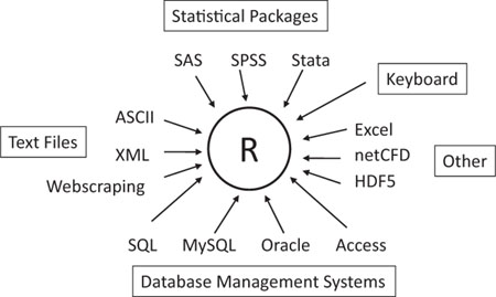
As you can see in figure 2.2, R can import data from the keyboard, from flat files, from Microsoft Excel and Access, from popular statistical packages, from specialty formats, and from a variety of relational database management systems. Because you never know where your data will come from, we’ll cover each of them here. You only need to read about the ones you’re going to be using.

Figure 2.2. Sources of data that can be imported into R

2.3.1. Entering data from the keyboard

Perhaps the simplest method of data entry is from the keyboard. The edit() function in R will invoke a text editor that will allow you to enter your data manually. Here are the steps involved:

1.  Create an empty data frame (or matrix) with the variable names and modes you want to have in the final dataset.

2.  Invoke the text editor on this data object, enter your data, and save the results back to the data object.

In the following example, you’ll create a data frame named mydata with three variables: age (numeric), gender (character), and weight (numeric). You’ll then invoke the text editor, add your data, and save the results.

mydata <- data.frame(age=numeric(0),
  gender=character(0), weight=numeric(0))
mydata <- edit(mydata)

Assignments like age=numeric(0) create a variable of a specific mode, but without actual data. Note that the result of the editing is assigned back to the object itself. The edit() function operates on a copy of the object. If you don’t assign it a destination, all of your edits will be lost!

The results of invoking the edit() function on a Windows platform can be seen in figure 2.3.

Figure 2.3. Entering data via the built-in editor on a Windows platform

In this figure, I’ve taken the liberty of adding some data. If you click on a column title, the editor gives you the option of changing the variable name and type (numeric, character). You can add additional variables by clicking on the titles of unused columns. When the text editor is closed, the results are saved to the object assigned (mydata in this case). Invoking mydata <- edit(mydata) again allows you to edit the data you’ve entered and to add new data. A shortcut for mydata <- edit(mydata) is simply fix(mydata).

This method of data entry works well for small datasets. For larger datasets, you’ll probably want to use the methods we’ll describe next: importing data from existing text files, Excel spreadsheets, statistical packages, or database management systems.

2.3.2. Importing data from a delimited text file

You can import data from delimited text files using read.table(), a function that reads a file in table format and saves it as a data frame. Here’s the syntax:

mydataframe <- read.table(file, header=logical_value,
  sep="delimiter", row.names="name")

where file is a delimited ASCII file, header is a logical value indicating whether the first row contains variable names (TRUE or FALSE), sep specifies the delimiter separating data values, and row.names is an optional parameter specifying one or more variables to represent row identifiers.

For example, the statement

grades <- read.table("studentgrades.csv", header=TRUE, sep=",",
  row.names="STUDENTID")

reads a comma-delimited file named studentgrades.csv from the current working directory, gets the variable names from the first line of the file, specifies the variable STUDENTID as the row identifier, and saves the results as a data frame named grades.

Note that the sep parameter allows you to import files that use a symbol other than a comma to delimit the data values. You could read tab-delimited files with sep=" ". The default is sep="", which denotes one or more spaces, tabs, new lines, or carriage returns.

By default, character variables are converted to factors. This behavior may not always be desirable (for example, a variable containing respondents’ comments). You can suppress this behavior in a number of ways. Including the option stringsAsFactors=FALSE will turn this behavior off for all character variables. Alternatively, you can use the colClasses option to specify a class (for example, logical, numeric, character, factor) for each column.

The read.table() function has many additional options for fine-tuning the data import. See help(read.table) for details.

 

Note

Many of the examples in this chapter import data from files that exist on the user’s computer. R provides several mechanisms for accessing data via connections as well. For example, the functions file(), gzfile(), bzfile(), xzfile(), unz(), and url() can be used in place of the filename. The file() function allows the user to access files, the clipboard, and C-level standard input. The gzfile(), bzfile(), xzfile(), and unz() functions let the user read compressed files. The url() function lets you access internet files through a complete URL that includes http://, ftp://, or file://. For HTTP and FTP, proxies can be specified. For convenience, complete URLs (surrounded by “” marks) can usually be used directly in place of filenames as well. See help(file) for details.

 

2.3.3. Importing data from Excel

The best way to read an Excel file is to export it to a comma-delimited file from within Excel and import it to R using the method described earlier. On Windows systems you can also use the RODBC package to access Excel files. The first row of the spreadsheet should contain variable/column names.

First, download and install the RODBC package.

install.packages("RODBC")

You can then use the following code to import the data:

library(RODBC)
channel <- odbcConnectExcel("myfile.xls")
mydataframe <- sqlFetch(channel, "mysheet")
odbcClose(channel)

Here, myfile.xls is an Excel file, mysheet is the name of the Excel worksheet to read from the workbook, channel is an RODBC connection object returned by odbcConnectExcel(), and mydataframe is the resulting data frame. RODBC can also be used to import data from Microsoft Access. See help(RODBC) for details.

Excel 2007 uses an XLSX file format, which is essentially a zipped set of XML files. The xlsx package can be used to access spreadsheets in this format. Be sure to download and install it before first use. The read.xlsx() function imports a worksheet from an XLSX file into a data frame. The simplest format is read.xlsx(file, n) where file is the path to an Excel 2007 workbook and n is the number of the worksheet to be imported. For example, on a Windows platform, the code

library(xlsx)
workbook <- "c:/myworkbook.xlsx"
mydataframe <- read.xlsx(workbook, 1)

imports the first worksheet from the workbook myworkbook.xlsx stored on the C: drive and saves it as the data frame mydataframe. The xlsx package can do more than import worksheets. It can create and manipulate Excel XLSX files as well. Programmers who need to develop an interface between R and Excel should check out this relatively new package.

2.3.4. Importing data from XML

Increasingly, data is provided in the form of files encoded in XML. R has several packages for handling XML files. For example, the XML package written by Duncan Temple Lang allows users to read, write, and manipulate XML files. Coverage of XML is beyond the scope of this text. Readers interested in the accessing XML documents from within R are referred to the excellent package documentation at www.omegahat.org/RSXML.

2.3.5. Webscraping

In webscraping, the user extracts information embedded in a web page available over the internet and saves it into R structures for further analysis. One way to accomplish this is to download the web page using the readLines() function and manipulate it with functions such as grep() and gsub(). For complex web pages, the RCurl and XML packages can be used to extract the information desired. For more information, including examples, see “Webscraping using readLines and RCurl,” available from the website Programming with R (www.programmingr.com).

2.3.6. Importing data from SPSS

SPSS datasets can be imported into R via the read.spss() function in the foreign package. Alternatively, you can use the spss.get() function in the Hmisc package. spss.get() is a wrapper function that automatically sets many parameters of read.spss() for you, making the transfer easier and more consistent with what data analysts expect as a result.

First, download and install the Hmisc package (the foreign package is already installed by default):

install.packages("Hmisc")

Then use the following code to import the data:

library(Hmisc)
mydataframe <- spss.get("mydata.sav", use.value.labels=TRUE)

In this code, mydata.sav is the SPSS data file to be imported, use.value.labels=TRUE tells the function to convert variables with value labels into R factors with those same levels, and mydataframe is the resulting R data frame.

2.3.7. Importing data from SAS

A number of functions in R are designed to import SAS datasets, including read.ssd() in the foreign package and sas.get() in the Hmisc package. Unfortunately, if you’re using a recent version of SAS (SAS 9.1 or higher), you’re likely to find that these functions don’t work for you because R hasn’t caught up with changes in SAS file structures. There are two solutions that I recommend.

You can save the SAS dataset as a comma-delimited text file from within SAS using PROC EXPORT, and read the resulting file into R using the method described in section 2.3.2. Here’s an example:

SAS program:

proc export data=mydata
     outfile="mydata.csv"
     dbms=csv;
run;

R program:

mydata <- read.table("mydata.csv", header=TRUE, sep=",")

Alternatively, a commercial product called Stat Transfer (described in section 2.3.12) does an excellent job of saving SAS datasets (including any existing variable formats) as R data frames.

2.3.8. Importing data from Stata

Importing data from Stata to R is straightforward. The necessary code looks like this:

library(foreign)
mydataframe <- read.dta("mydata.dta")

Here, mydata.dta is the Stata dataset and mydataframe is the resulting R data frame.

2.3.9. Importing data from netCDF

Unidata’s netCDF (network Common Data Form) open source software contains machine-independent data formats for the creation and distribution of array-oriented scientific data. netCDF is commonly used to store geophysical data. The ncdf and ncdf4 packages provide high-level R interfaces to netCDF data files.

The ncdf package provides support for data files created with Unidata’s netCDF library (version 3 or earlier) and is available for Windows, Mac OS X, and Linux platforms. The ncdf4 package supports version 4 or earlier, but isn’t yet available for Windows.

Consider this code:

library(ncdf)
nc <- nc_open("mynetCDFfile")
myarray <- get.var.ncdf(nc, myvar)

In this example, all the data from the variable myvar, contained in the netCDF file mynetCDFfile, is read and saved into an R array called myarray.

Note that both ncdf and ncdf4 packages have received major recent upgrades and may operate differently than previous versions. Additionally, function names in the two packages differ. Read the online documentation for details.

2.3.10. Importing data from HDF5

HDF5 (Hierarchical Data Format) is a software technology suite for the management of extremely large and complex data collections. The hdf5 package can be used to write R objects into a file in a form that can be read by software that understands the HDF5 format. These files can be read back into R at a later time. The package is experimental and assumes that the user has the HDF5 library (version 1.2 or higher) installed. At present, support for the HDF5 format in R is extremely limited.

2.3.11. Accessing database management systems (DBMSs)

R can interface with a wide variety of relational database management systems (DBMSs), including Microsoft SQL Server, Microsoft Access, MySQL, Oracle, PostgreSQL, DB2, Sybase, Teradata, and SQLite. Some packages provide access through native database drivers, whereas others offer access via ODBC or JDBC. Using R to access data stored in external DMBSs can be an efficient way to analyze large datasets (see appendix G), and leverages the power of both SQL and R.

The ODBC Interface

Perhaps the most popular method of accessing a DBMS in R is through the RODBC package, which allows R to connect to any DBMS that has an ODBC driver. This includes all of the DBMSs listed.

The first step is to install and configure the appropriate ODBC driver for your platform and database—they’re not part of R. If the requisite drivers aren’t already installed on your machine, an internet search should provide you with options.

Once the drivers are installed and configured for the database(s) of your choice, install the RODBC package. You can do so by using the install.packages("RODBC") command.

The primary functions included with the RODBC package are listed in table 2.2.

Table 2.2. RODBC functions

Function	Description
odbcConnect(dsn,uid="",pwd="")	Open a connection to an ODBC database
sqlFetch(channel,sqltable)	Read a table from an ODBC database into a data frame
sqlQuery(channel,query)	Submit a query to an ODBC database and return the results
sqlSave(channel,mydf, tablename = sqtable, append=FALSE)	Write or update (append=TRUE) a data frame to a table in the ODBC database
sqlDrop(channel,sqtable)	Remove a table from the ODBC database
close(channel)	Close the connection

The RODBC package allows two-way communication between R and an ODBC-connected SQL database. This means that you can not only read data from a connected database into R, but you can use R to alter the contents of the database itself. Assume that you want to import two tables (Crime and Punishment) from a DBMS into two R data frames called crimedat and pundat, respectively. You can accomplish this with code similar to the following:

library(RODBC)
myconn <-odbcConnect("mydsn", uid="Rob", pwd="aardvark")
crimedat <- sqlFetch(myconn, Crime)
pundat <- sqlQuery(myconn, "select * from Punishment")
close(myconn)

Here, you load the RODBC package and open a connection to the ODBC database through a registered data source name (mydsn) with a security UID (rob) and password (aardvark). The connection string is passed to sqlFetch, which copies the table Crime into the R data frame crimedat. You then run the SQL select statement against the table Punishment and save the results to the data frame pundat. Finally, you close the connection.

The sqlQuery() function is very powerful because any valid SQL statement can be inserted. This flexibility allows you to select specific variables, subset the data, create new variables, and recode and rename existing variables.

DBI-Related Packages

The DBI package provides a general and consistent client-side interface to DBMS. Building on this framework, the RJDBC package provides access to DBMS via a JDBC driver. Be sure to install the necessary JDBC drivers for your platform and database. Other useful DBI-based packages include RMySQL, ROracle, RPostgreSQL, and RSQLite. These packages provide native database drivers for their respective databases but may not be available on all platforms. Check the documentation on CRAN (http://cran.r-project.org) for details.

2.3.12. Importing data via Stat/Transfer

Before we end our discussion of importing data, it’s worth mentioning a commercial product that can make the task significantly easier. Stat/Transfer (www.stattransfer.com) is a stand-alone application that can transfer data between 34 data formats, including R (see figure 2.4).

Figure 2.4. Stat/Transfer’s main dialog on Windows

It’s available for Windows, Mac, and Unix platforms and supports the latest versions of the statistical packages we’ve discussed so far, as well as ODBC-accessed DBMSs such as Oracle, Sybase, Informix, and DB/2.

2.4. Annotating datasets

Data analysts typically annotate datasets to make the results easier to interpret. Typically annotation includes adding descriptive labels to variable names and value labels to the codes used for categorical variables. For example, for the variable age, you might want to attach the more descriptive label “Age at hospitalization (in years).” For the variable gender coded 1 or 2, you might want to associate the labels “male” and “female.”

2.4.1. Variable labels

Unfortunately, R’s ability to handle variable labels is limited. One approach is to use the variable label as the variable’s name and then refer to the variable by its position index. Consider our earlier example, where you have a data frame containing patient data. The second column, named age, contains the ages at which individuals were first hospitalized. The code

names(patientdata)[2] <- "Age at hospitalization (in years)"

renames age to "Age at hospitalization (in years)". Clearly this new name is too long to type repeatedly. Instead, you can refer to this variable as patientdata[2] and the string "Age at hospitalization (in years)" will print wherever age would’ve originally. Obviously, this isn’t an ideal approach, and you may be better off trying to come up with better names (for example, admissionAge).

2.4.2. Value labels

The factor() function can be used to create value labels for categorical variables. Continuing our example, say that you have a variable named gender, which is coded 1 for male and 2 for female. You could create value labels with the code

patientdata$gender <- factor(patientdata$gender,
                             levels = c(1,2),
                             labels = c("male", "female"))

Here levels indicate the actual values of the variable, and labels refer to a character vector containing the desired labels.

2.5. Useful functions for working with data objects

We’ll end this chapter with a brief summary of useful functions for working with data objects (see table 2.3).

Table 2.3. Useful functions for working with data objects

Function	Purpose
length(object)	Number of elements/components.
dim(object)	Dimensions of an object.
str(object)	Structure of an object.
class(object)	Class or type of an object.
mode(object)	How an object is stored.
names(object)	Names of components in an object.
c(object, object,...)	Combines objects into a vector.
cbind(object, object, ...)	Combines objects as columns.
rbind(object, object, ...)	Combines objects as rows.
object	Prints the object.
head(object)	Lists the first part of the object.
tail(object)	Lists the last part of the object.
Is()	Lists current objects.
rm(object, object, ...)	Deletes one or more objects. The statement rm(list = Is()) will remove most objects from the working environment.
newobject <- edit(object)	Edits object and saves as newobject.
fix(object)	Edits in place.

We’ve already discussed most of these functions. The functions head() and tail() are useful for quickly scanning large datasets. For example, head(patientdata) lists the first six rows of the data frame, whereas tail(patientdata) lists the last six. We’ll cover functions such as length(), cbind(), and rbind() in the next chapter. They’re gathered here as a reference.

2.6. Summary

One of the most challenging tasks in data analysis is data preparation. We’ve made a good start in this chapter by outlining the various structures that R provides for holding data and the many methods available for importing data from both keyboard and external sources. In particular, we’ll use the definitions of a vector, matrix, data frame, and list again and again in later chapters. Your ability to specify elements of these structures via the bracket notation will be particularly important in selecting, subsetting, and transforming data.

As you’ve seen, R offers a wealth of functions for accessing external data. This includes data from flat files, web files, statistical packages, spreadsheets, and databases. Although the focus of this chapter has been on importing data into R, you can also export data from R into these external formats. Exporting data is covered in appendix C, and methods of working with large datasets (in the gigabyte to terabyte range) are covered in appendix G.

Once you get your datasets into R, it’s likely that you’ll have to manipulate them into a more conducive format (actually, I find guilt works well). In chapter 4, we’ll explore ways of creating new variables, transforming and recoding existing variables, merging datasets, and selecting observations.

But before turning to data management tasks, let’s spend some time with R graphics. Many readers have turned to R out of an interest in its graphing capabilities, and I don’t want to make you wait any longer. In the next chapter, we’ll jump directly into the creation of graphs. Our emphasis will be on general methods for managing and customizing graphs that can be applied throughout the remainder of this book.