We are now ready to build our classification model on the features we extracted in the previous section. The code for this section is available in the Modeling.ipynb Jupyter Notebook in case you want to run the examples yourself. To start, let's load some essential dependencies:
from sklearn.externals import joblib
import keras
from keras import models
from keras import layers
import model_evaluation_utils as meu
import matplotlib.pyplot as plt

%matplotlib inline
We will use our nifty model evaluation utilities module named model_evaluation_utils to evaluate our classifier and test its performance later on. Let's load up our feature sets and data point class labels now:
train_features = joblib.load('train_tl_features.pkl')
train_labels = joblib.load('train_labels.pkl')
validation_features = joblib.load('validate_tl_features.pkl')
validation_labels = joblib.load('validate_labels.pkl')
test_features = joblib.load('test_tl_features.pkl')
test_labels = joblib.load('test_labels.pkl')
train_features.shape, validation_features.shape, test_features.shape

((18300, 2048), (6100, 2048), (6100, 2048))


train_labels.shape, validation_labels.shape, test_labels.shape

((18300,), (6100,), (6100,))
Thus, we can see that all our feature sets and corresponding labels have been loaded. The input feature sets are one-dimensional vectors of size 2,048 obtained from the VGG-16 model we used in the previous section. We now need to one-hot encode the categorical class labels before we can feed them to a deep learning model. The following snippet helps us achieve this:
from keras.utils import to_categorical
train_labels_ohe = to_categorical(train_labels)
validation_labels_ohe = to_categorical(validation_labels)
test_labels_ohe = to_categorical(test_labels)
train_labels_ohe.shape, validation_labels_ohe.shape, test_labels_ohe.shape

((18300, 10), (6100, 10), (6100, 10))
We will now build our deep learning classifier by using a fully connected network that has four hidden layers. We will use the usual components like dropout to prevent overfitting and the Adam optimizer for our model. Details of the model architecture are depicted in the following code:
model = models.Sequential()
model.add(layers.Dense(1024, activation='relu',
          input_shape=(train_features.shape[1],)))
model.add(layers.Dropout(0.4))
model.add(layers.Dense(1024, activation='relu'))
model.add(layers.Dropout(0.4))
model.add(layers.Dense(512, activation='relu'))
model.add(layers.Dropout(0.5))
model.add(layers.Dense(512, activation='relu'))
model.add(layers.Dropout(0.5))
model.add(layers.Dense(train_labels_ohe.shape[1],activation='softmax'))
model.compile(loss='categorical_crossentropy',
              optimizer='adam',metrics=['accuracy'])
model.summary()


_________________________________________________________________
Layer (type)                 Output Shape              Param #
=================================================================
dense_1 (Dense)              (None, 1024)              2098176
_________________________________________________________________
dropout_1 (Dropout)          (None, 1024)              0
_________________________________________________________________
dense_2 (Dense)              (None, 1024)              1049600
_________________________________________________________________
dropout_2 (Dropout)          (None, 1024)              0
_________________________________________________________________
dense_3 (Dense)              (None, 512)               524800
_________________________________________________________________
dropout_3 (Dropout)          (None, 512)               0
_________________________________________________________________
dense_4 (Dense)              (None, 512)               262656
_________________________________________________________________
dropout_4 (Dropout)          (None, 512)               0
_________________________________________________________________
dense_5 (Dense)              (None, 10)                5130
=================================================================

Total params: 3,940,362
Trainable params: 3,940,362
Non-trainable params: 0
This model was then trained on an AWS p2.x instance for about fifty epochs with a batch size of 128. We recommend a GPU to train this model; you can play around with the epochs and batch size to get a robust model, as follows:
history = model.fit(train_features, train_labels_ohe,epochs=50,
                    batch_size=128,
                    validation_data=(validation_features,
                    validation_labels_ohe),shuffle=True, verbose=1)
Train on 18300 samples, validate on 6100 samples
Epoch 1/50
18300/18300 - 2s - loss: 2.7953 - acc: 0.3959 - val_loss: 1.0665 - val_acc: 0.6675
Epoch 2/50
18300/18300 - 1s - loss: 1.1606 - acc: 0.6211 - val_loss: 0.8179 - val_acc: 0.7444
...
...
Epoch 48/50
18300/18300 - 1s - loss: 0.2753 - acc: 0.9157 - val_loss: 0.4218 - val_acc: 0.8797
Epoch 49/50
18300/18300 - 1s - loss: 0.2813 - acc: 0.9142 - val_loss: 0.4220 - val_acc: 0.8810
Epoch 50/50
18300/18300 - 1s - loss: 0.2631 - acc: 0.9197 - val_loss: 0.3887 - val_acc: 0.8890
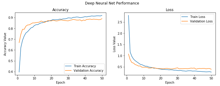
We get a validation accuracy of close to 89%, which is pretty good and things look promising. We can also plot the overall accuracy and loss plots of the model to get a better idea of what things look like, as follows:
f, (ax1, ax2) = plt.subplots(1, 2, figsize=(12, 4))
t = f.suptitle('Deep Neural Net Performance', fontsize=12)
f.subplots_adjust(top=0.85, wspace=0.2)
epochs = list(range(1,51))
ax1.plot(epochs, history.history['acc'], label='Train Accuracy')
ax1.plot(epochs, history.history['val_acc'], label='Validation Accuracy')
ax1.set_ylabel('Accuracy Value')
ax1.set_xlabel('Epoch')
ax1.set_title('Accuracy')
l1 = ax1.legend(loc="best")
ax2.plot(epochs, history.history['loss'], label='Train Loss')
ax2.plot(epochs, history.history['val_loss'], label='Validation Loss')
ax2.set_ylabel('Loss Value')
ax2.set_xlabel('Epoch')
ax2.set_title('Loss')
l2 = ax2.legend(loc="best")
This will create the following plots:

We can see that the model's loss and accuracy between training and validation is quite consistent; maybe it overfits slightly, but it is negligible considering their difference is quite low.
