

The IBM General Parallel File System for technical cloud computing
This chapter describes technical aspects of the IBM General Parallel File System (GPFS) that make it a good file system choice for technical computing clouds.
This chapter includes the following sections:
This chapter also introduces the following new GPFS functions:
6.1 Overview
The IBM General Parallel File System (GPFS) has many characteristics that make it a good choice for the file system within technical computing environments and technical computing clouds. GPFS helps ease the management of the file system, ensure performance, and helps ensure concurrent access to data. The following is a list of the GPFS characteristics:
•High capacity
•High performance
•High availability
•Single-system image
•Multiple operating system and server architecture support
•Parallel data access
•Clustering of nodes
•Shared disks architecture
Each one of these characteristics is described in the following sections.
6.1.1 High capacity
GPFS is able to span a larger number of disks than other conventional file systems. This means that the final file system size that you can reach with it is larger. When you consider a technical computing environment for data intensive workloads, that extra space can make a difference. When you consider a cloud environment where you can deploy multiple technical computing environment workloads, the ability scale up and easily grow the file system size becomes important.
Currently, the maximum size a GPFS file system can reach is 512 XB (xonabytes), which is equal to 299 bytes. The maximum number of files that can be stored in a single GPFS file system is 263 files. That is 8 millions of trillions of files. Regarding disk size, the limit is imposed solely by the disk and operating system device drivers.
6.1.2 High performance
GPFS is built to provide performance to file access. I/O operations to a file in technical computing environments must happen efficiently. This is because files can be large, or many of them must be accessed at a time. To accomplish this, GPFS uses a few techniques to store the data:
•Large block size and full-stride I/O
•Wide striping: Spread a file over all disks
•Parallel multi-node I/O
•I/O multithreading
•Intelligent pre-fetch and file caching algorithms
•Access pattern optimization
6.1.3 High availability
Large technical computing environments and clouds must be highly available and eliminate single points of failure. GPFS embeds this characteristic by keeping metadata and logs, ensuring these are always available to the participating cluster nodes (for example, log replication), and by applying disk lease mechanisms (heartbeat).
If a node in a GPFS cluster fails, the log of the failed node can be replayed on the file system manager node.
Recoverability from failure situations is not the only way GPFS ensures high availability. High availability is also obtained with a correct disk access layout. Multiple GPFS server nodes can access the storage LUNs and serve the data. Also, the servers themselves access the LUNs through redundant paths. Moreover, each of the GPFS server nodes can access all of the LUNs. A clearer definition and understanding of high availability file system layout point of view can be found in 6.2, “GPFS layouts for technical computing” on page 115.
In addition, GPFS offers management capabilities that do not require downtime. These include the addition or removal of disks, and addition or removal of nodes in the GPFS cluster, which all can be performed without having to unmount the target file system.
6.1.4 Single system image
A GPFS file system is different from, say, an NFS one, as it can be seen as the same file system on each of the participating nodes. With NFS, the file system belongs to the node that serves that file system, and other nodes connect to it. In GPFS, there is no concept of a file system-owning node within the same GPFS cluster. All of the cluster nodes have global access to data on the file system.
It is also possible to create cross-cluster-mount scenarios where one GPFS cluster owns the file system and serves it to another remote cluster over the network. This is described in 6.2, “GPFS layouts for technical computing” on page 115.
This characteristic of GPFS simplifies operations and management, and allows nodes in different geographical locations to see the same file system and data, which is a benefit for a technical computing cloud environment.
6.1.5 Multiple operating system and server architecture support
The GPFS file system can be accessed by a multitude of operating systems. The supported operating systems for GPFS version 3.5 TL3 are shown in Table 6-1. Earlier releases of GPFS support older operating system versions. For an up-to-date list of supported operating systems, see:
Table 6-1 GPFS 3.5 TL3 operating systems support
|
Operating system
|
Versions
|
|
IBM AIX
|
6.1, 7.1
|
|
RedHat Enterprise Linux
|
5, 6
|
|
SUSE Linux Enterprise Server
|
10, 11
|
|
Microsoft Windows 2007 Server
|
Enterprise and Ultimate editions
|
|
Microsoft Windows 2008 Server
|
R1 (SP2), R2
|
Also, the following multiple server architectures are supported:
•IBM POWER
•x86 architecture
– Intel EM64T
– AMD Opteron
– Intel Pentium 3 or newer processor
•Intel Itanium 2
This broad support allows the creation of technical computing environments that use different hardware server architectures (POWER, Intel-based servers, virtual machines) besides support for multiple operating systems. Therefore, GPFS is positioned to be the common file system of a multi-hardware, multi-purpose technical computing cloud environment.
6.1.6 Parallel data access
File systems are traditionally able to allow safe, concurrent access to a file, but it usually happens in a sequential form, that is, one task or one I/O request at a time.
GPFS uses a much more fine-grained approach that is based on byte range locking, a mechanism that is facilitated by the use of tokens. An I/O operation can access a byte range within a file if it holds a token for that byte range. By organizing data access in byte ranges and using tokens to grant access to it, different applications can access the same file at the same time, if they aim to access a different byte range of that file. This increases parallelism while still ensuring data integrity. The management of the data in byte ranges is transparent to the user or application.
Also, data placement on disks, multiple cluster node access to disks, and data striping and striding strategies allow GPFS to access different chunks of the data in parallel.
6.1.7 Clustering of nodes
GPFS supports clustering of nodes up to 8192 nodes. This benefits technical computing clouds that can be composed of thousands of nodes as well.
6.1.8 Shared disks architecture
GPFS uses a shared disk architecture that allows data and metadata to be accessible by any of the nodes within the GPFS cluster. This allows the system to achieve parallel access to data and increase performance.
The sharing of disks can happen in either a direct disk connection (a storage LUN is mapped to multiple cluster nodes) or by using the GPFS Network Shared Disk (NSD) protocol over the network (TCP/IP of InfiniBand). A direct disk connection provides the best performance, but might not suit all the technical scenarios. These different layouts are explained in 6.2, “GPFS layouts for technical computing” on page 115.
Because a technical computing cloud environment might be diverse in its hardware infrastructure and hardware components, GPFS provides flexibility while maintaining performance and parallelism to data access.
6.2 GPFS layouts for technical computing
For Technical Computing, GPFS can provide various cluster configurations independent of which file system features you use. There are four basic layouts for the GPFS cluster configurations within a Technical Computing cloud:
•Shared disk
•Network block I/O
•Mixed cluster
•Sharing data between clusters
6.2.1 Shared disk
In a shared disk cluster layout, nodes can all be directly attached to a common SAN storage as shown in Figure 6-1. This means that all nodes can concurrently access each shared block device in the GPFS cluster through a block level protocol.

Figure 6-1 SAN-attached storage
Figure 6-1 shows that the GPFS cluster nodes are connected to the storage over the SAN and to each other over the LAN. It shows a Fibre Channel SAN through the storage attachment technology, which can be InfiniBand, SAS, FCoE or any other. Data that are used by applications that run on the GPFS nodes flow over the SAN and the GPFS control information flows among the GPFS instances in the cluster over the LAN. This is a good configuration for providing network file service to client systems using clustered NFS, high-speed data access for digital media applications, or a grid infrastructure for data analytics.
6.2.2 Network block I/O
In environments where you do not have to adopt a single SAN storage technology attached to every node in the cluster, a block level interface over Internet Protocol networks called the NSD protocol can be an option. GPFS clusters can use NSD server nodes to remotely serve disk data to other NSD client nodes. NSD is a disk level virtualization.
In this configuration, disks are attached only to the NSD servers. Within Technical Computing clouds, you can use NSD protocol in GPFS clusters to provide high speed data access for applications that run on NSD client nodes. To avoid a single point of server failure, define at least two NSD servers for each disk as shown in Figure 6-2.

Figure 6-2 Network block I/O
Network block I/O is better for clusters with sufficient network bandwidth between NSD servers and clients. Figure 6-2 shows an example of a network block I/O configuration where NSD clients are connected to NSD servers through a high speed interconnect or an IP-based network such as Ethernet. Figure 6-2 also illustrates that data flows from the storage to the NSD servers over the SAN, and then flows from the NSD servers to the NSD clients across the LAN. NSD clients see the local block I/O devices, same as directly attached, and remote I/O is transparent to the applications. The parallel data access provides the best possible throughput to all clients.
The choice between SAN attachment and network block I/O are performance and costs. In general, using a SAN provides the highest performance; but the cost and management complexity of SANs for large clusters is often prohibitive. In these cases, network block I/O provides an option. For example, a grid is effective for statistical applications such as financial fraud detection, supply chain management or data mining.
6.2.3 Mixed clusters
Based on the previous two sections, you can also mix direct SAN and NSD attachment topologies in GPFS clusters. Figure 6-3 shows some application nodes (with high bandwidth) are directly attached to the SAN while other application nodes are attached to the NSD servers. This mix implementation makes a cluster configuration flexible and provides better I/O throughput to meet the application requirements. In addition, this mix cluster architecture enables high performance access to a common set of data to support a scale-out solution and to provide a high available platform.
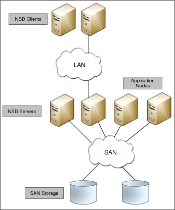
Figure 6-3 Mixed cluster architecture
A GPFS node always tries to find the most efficient path to the storage. If a node detects a block device path to the data, this path is used. If there is no block device path, the network is used. This capability is used to provide extra availability. If a node is SAN-attached to the storage and there is an HBA failure, for example, GPFS can fail over and use the network path to the disk. A mixed cluster topology can provide direct storage access to non-NSD server nodes for high performance operations, including backups.
6.2.4 Sharing data between clusters
There are two ways available to share data between GPFS clusters: GPFS multi-cluster and Active File Management (AFM). GPFS multi-clusters allow GPFS nodes to natively mount a GPFS file system from another GPFS cluster.
A multi-cluster file system features extreme scalability and throughput that is optimized for streaming workloads such as those common in web 2.0, digital media, scientific, and engineering applications. Users shared access to files in either the cluster where the file system was created, or other GPFS clusters. Each site in the network is managed as a separate cluster, while still allowing shared file system access.
GPFS multi-clusters allow you to use the native GPFS protocol to share data across clusters. With this feature, you can allow other clusters to access one or more of your file systems. You can also mount and have access to file systems that belong to other clusters for which you have been authorized access. Thus, multi-clusters demonstrate the viability and usefulness of a global file system, but also reduce the need for multiple data copies. Figure 6-4 shows a multi-cluster configuration with both LAN and mixed LAN and SAN topologies.

Figure 6-4 Multi-cluster
As shown in Figure 6-4, Cluster A owns the storage and manages the file system. Remote clusters such as Cluster B and Cluster C that do not have any storage are able to mount and access, if they are authorized, the file system from Cluster A. Cluster B accesses the data through the NSD protocol over the LAN, whereas Cluster C accesses the data over an extension of the SAN.
Multi-clusters can share data across clusters that belong to different organizations for collaborative computing, grouping sets of clients for administrative purposes, or implementing a global namespace across separate locations. A multi-cluster configuration connects GPFS clusters within a data center, across a campus, or across reliable WAN links. To share data between GPFS clusters across less reliable WAN links or in cases where you want a copy of the data in multiple locations, you can use a new feature introduced in GPFS 3.5 called AFM. For more information, see 6.4.1, “Active File Management (AFM)” on page 124.
6.3 Integration with IBM Platform Computing products
To help solve challenges in Technical Computing clouds, IBM GPFS has implemented integrations with IBM Platform Computing products such as IBM Platform Cluster Manager - Advanced Edition (PCM-AE) and Platform Symphony.
6.3.1 IBM Platform Cluster Manager - Advanced Edition (PCM-AE)
PCM-AE integrates with GPFS, which provisions secure multi-tenant high-performance computing (HPC) clusters that are created with secure GPFS storage mounted on each server. Storage is secure because only authorized cloud users can access storage that is assigned to their accounts. You can use GPFS for PCM-AE as an extended storage that looks like one folder in the operating system for virtual machines or physical systems. Or you can use GPFS for PCM-AE as an image (raw, qcow2) storage repository for virtual machines.
Considerations
There are some considerations to have in mind before you implement GPFS for PCM-AE secure storage:
•The GPFS package URL. This is specified to create the GPFS storage adapter instance.
•GPFS connects to the provisioning (private) network
•Configure SSH passwordless logon
•Configure the SSH and SCP remote commands
•Install the expect command
•Enable the GPFS adminMode configuration parameter
•Allow access to the GPFS port (1191)
•Select the GPFS master
•Ensure that the GPFS master's host name resolves
•Install the LDAP client on the GPFS master and NSD server
•Disable the GPFS automatic mount flag
For GPFS performance tuning in Technical Computing clouds environments, you can disable the GSSAPIAuthentication and UseDNS settings in the ssh configuration file on the GPFS master within PCM-AE environments.
Usability and administration
This section describes usability and administration examples for GPFS in a PCM-AE cloud environment. In GPFS, you can add a GPFS storage adapter instance, and then create, delete, assign, or unassign storage for GPFS. You can even create a cluster definition with GPFS. The following list gives an administration summary for GPFS:
•Add a GPFS storage adapter instance
•Add storage
•Delete storage
•Assign storage to accounts
•Unassign storage from accounts
•Create a cluster definition with GPFS
•Instantiate a cluster definition with nodes mounting GPFS
•Troubleshoot GPFS storage
For more information about GPFS administration, see the “Secure storage using a GPFS cluster file system” chapter in Platform Cluster Manager Advanced Edition Version 4 Release 1: Administering, SC27-4760-01.
Integration summary
Cloud administrators must add a storage adapter instance, then go to the GUI page of a specific storage adapter instance to create storage through this adapter.
After storage is assigned to an account, all the users/groups of this account are given the permissions (read, write, execution, and rwx) to access the storage. To achieve this, PCM-AE communicates with the GPFS master node to add user/group to the access control list (ACL) for the related directory in the GPFS file system.
The machine definition author enables the GPFS storage, and can add only one GPFS storage to each machine layer. The storage that is selected in the machine definition is used for the GPFS postscript layer.
Figure 6-5 shows the resulting PCM-AE GUI after you select Resources → Inventory → GPFS → storage_adapter_instance (c445gpfs2). Click the Storage tab and select the storage that you want to assign to an account (Figure 6-5).
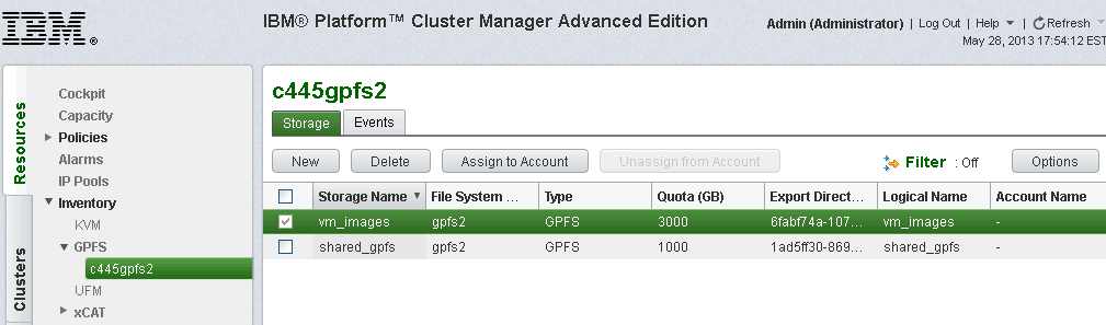
Figure 6-5 Storage tab in PCM-AE
Cloud administrators can define the cluster definition, and select Storage1 for its machine layer, then publish it and instantiate this cluster definition. The machine definition author can specify a mount point. The mount point is a link path to the real storage under the GPFS file system. This is to be consistent with other shared storage.
The GPFS file system that contains the storage is mounted on the machines in tiers that contain the GPFS internal postscript layer. The postscript layer is an internal postscript layer that PCM-AE runs. Even if implemented as an internal postscript layer, you still must specify the location of the GPFS client packages by the GPFS package URL when you create the GPFS storage adapter instance.
|
Tip: When the cluster machines are provisioned with the GPFS file system that contains the storage, the user is not required to manually mount the file system.
|
The GPFS storage that is assigned to the account defaults to the mount point /gpfs. A subdirectory with the cluster ID as its directory name is created in the storage (by the local system command mkdir), and linked to the “mount point” that the user specifies. Therefore, the user can access this subdirectory with the path of “mount point”. All these steps run in the GPFS internal postscript layer.
Figure 6-6 shows how the cluster machines provisioned by PCM-AE work with the GPFS cluster.

Figure 6-6 PCM-AE and GPFS
The cluster shares the FileSysName/ExportDirectory directory in the GPFS file system. The example shown in Figure 6-6 shows two accounts: Account1 and Account2. Storage1 and Storage2 are two storages that were created by the administrator. Storage1 is assigned to Account1, and Storage2 is assigned to Account2. For Storage1, its file system name is fs1, and for Storage2, its file system name is fs2. For both of them, the export directory is data.
Account1 instantiates the cluster definition Def1_inst1 and specifies /foo as a mount point for Machine1 and Machine2. Account1 also instantiates the cluster definition Def2_inst1 and specifies /bar as a mount point for Machine3. Similarly, Account2 instantiates the cluster definition Def1_inst2 and specifies /foo as a mount point for Machine4 and Machine5. Account2 also instantiates the cluster definition Def2_inst2 and specifies /bar as a mount point for Machine6. If you want to have its private folder in the cluster, you can create it in its own postscript layer.
Current considerations
In the integration between PCM-AE and GPFS, keep these considerations in mind:
•The GPFS cluster must use the same LDAP server with the PCM-AE master so that they can share the user database.
•One GPFS master cannot be shared by multiple PCM-AE environments.
•The GPFS master and the cluster must be set up and ready before you start client provisioning.
•There is a network route between the virtual machines, physical machines, the xCAT management node, the PCM-AE master, the KVM hypervisor, and the GPFS master/NSD server.
•xCAT is the DNS server for the GPFS master, virtual machines, and physical machines.
6.3.2 IBM Platform Symphony
With IBM InfoSphere BigInsights 2.1, IBM is bringing new capabilities to Hadoop and providing tight integrations to solve many challenges of data management, scheduling efficiency and cluster management.
IBM Platform Symphony and GPFS are included in the IBM InfoSphere BigInsights reference architecture, which can be also supported with IBM Power Linux. The integration between Platform Symphony and GPFS overcomes several specific limitations of Hadoop to meet the big data analytics demands under a Technical Computing clouds, because the high performance scheduler combined with the high performance file system can compliment to deliver the ultimate analytics environment. The integration of IBM Platform Symphony and IBM GPFS provides service-oriented high-performance grid manager with low-latency scheduling and advanced resource-sharing capabilities, and delivering an enterprise-class POSIX file system.
IBM InfoSphere BigInsights 2.1 and GPFS File Placement Optimizer (FPO) features provide users with an alternative to HDFS. The implementation brings POSIX compliance and no single point of failure file system, thus replacing standard HDFS in MapReduce environments.
GPFS FPO delivers a set of features that extend GPFS providing Hadoop-style data-aware scheduling on a shared-nothing environment (meaning cluster nodes with local disk). A GPFS “connector” component included in IBM InfoSphere BigInsights (and also in GPFS) provides BigInsights customers with several advantages. For details, see 6.4.2, “File Placement Optimizer (FPO)” on page 129.
|
Note: GPFS FPO version 3.5.0.9 has been certified for use with Apache Hadoop 1.1.1 (the same version of Hadoop on which IBM InfoSphere BigInsights 2.1 is based). Platform Symphony 6.1.0.1 has also been tested with open source Hadoop 1.1.1. The necessary connector to emulate HDFS operations on GPFS FPO is included as part of the GPFS software distribution.
|
Layout
Figure 6-7 illustrates the implementation of the application adapter within the MapReduce framework in IBM Platform Symphony, and the integration between GPFS and Platform Symphony.

Figure 6-7 Integration between GPFS and Platform Symphony
Existing Hadoop MapReduce applications call the same Hadoop MapReduce and common library APIs. Hadoop-compatible MapReduce applications, however, can talk to and run on Platform Symphony, instead of on the Hadoop JobTracker and TaskTracker, through the MapReduce application adapter as shown in Figure 6-7. Both Hadoop MapReduce applications and the application adapter still call the Hadoop common library for distributed file systems such as HDFS and GPFS configurations.
The MapReduce framework in Platform Symphony also provides storage connectors to integrate with different file and database systems such as GPFS and Network File System (NFS). In the middle, the MapReduce application adapter and storage connectors are aware of both Hadoop and Platform Symphony systems.
Procedure
GPFS is a high-performance shared-disk file system that can provide fast data access from all nodes in a homogeneous or heterogeneous cluster of servers. The MapReduce framework in Platform Symphony provides limited support for running MapReduce jobs using GPFS 3.4 for data input, output, or both. For this purpose, the MapReduce framework in Platform Symphony includes a GPFS adapter (gpfs-pmr.jar) for the generic DFS interface, which is in the distribution lib directory.
The current MapReduce adapter for GPFS does not apply any data locality preferences to the MapReduce job's task scheduling. All data are considered equally available locally from any compute host. Large input files are still processed as multiple data blocks by different Map tasks (by default, the block size is set to 32 MB). Complete these steps to configure the GPFS adapter and run MapReduce jobs with it:
•Configure the GPFS cluster and start it (for more information, see the IBM General Parallel File System Version 3 Release 5.0.7: Advanced Administration Guide, SC23-5182-07). Mount the GPFS file system to the same local path for the MapReduce client and all compute hosts (for example, /gpfs).
•Merge the sample $PMR_HOME/conf/pmr-site.xml.gpfs file to the general configuration file $PMR_HOME/conf/pmr-site.xml on all the hosts. Restart the related MapReduce applications by disabling or enabling the applications.
•Use the GPFS adapter by specifying the gpfs:/// schema in the data input path, output path, or both. For example, if input data files in GPFS are mounted under local path /gpfs/input/ and you want to store the MapReduce job's result in GPFS mounted under the local path /gpfs/output, submit a MapReduce job by using the following syntax:
mrsh jar jarfile gpfs:///gpfs/input gpfs:///gpfs/output
6.4 GPFS features for Technical Computing
This section contains key features to support technical computing.
6.4.1 Active File Management (AFM)
Active File Management (AFM) is a distributed file caching feature in GPFS that allows the expansion of the GPFS global namespace across geographical distances. AFM helps provide a solution through enabling data sharing when wide area network connections are slow or not reliable for Technical Computing clouds.
AFM Architecture
AFM uses a home-and-cache model in which a single home provides the primary data storage, and exported data is cached in a local GPFS file system. Also, AFM can share data among multiple clusters running GPFS to provide a uniform name space and automate data movement (Figure 6-8 on page 125).
Home
Home can be thought of as any NFS mount point that is designated as the owner of the data in a cache relationship. Home can also be a GPFS cluster that has an NFS exported file system or independent file set. As the remote cluster or a collection of one or more NFS servers that cache connects to, only one Home exists in a cache relationship to provides the main storage for the data.
Cache
Cache is a kind of GPFS file set, and can be thought of as the container used to cache the home data. Each AFM-enabled file set cache is associated with a file set at home. File data is copied into a cache when requested. Whenever a file is read, if the file is not in cache or is not up to date, its data is copied into the cache from home. There are one or more gateway nodes as the cache is handling the cache traffic and communicating with home. Data that are written to cache are queued at the gateway node and then automatically pushed to home as quickly as possible.
In the AFM architecture (Figure 6-8), there are two Cache clusters sites and one Home cluster site. AFM minimizes the amount of traffic that is sent over the WAN. When Cache is disconnected from Home, cached files can be read, and new files and cached files can be written locally. This function provides high availability to Technical Computing clouds users. Also, cloud user access to the global file system goes through the Cache and they can see local performance if a file or directory is in the Cache.

Figure 6-8 AFM architecture
Supported features
AFM supports many features, which include the following:
•File set granularity. Different file sets at cache sites can link to different homes. Each exported home file set is cached by multiple cache sites.
•Persistent, scalable, read and write caching. Whole file, metadata, and namespace caching on demand. Configurable to be read-only or cache write only.
•Standard transport protocol between sites. NFSv3 is supported.
•Continued operations when network is disconnected. Automatic detection of network outage.
•Timeout-based cache revalidation. Configurable per object type per file set.
•Tunable delayed write-back to home. Configurable delayed writeback with command-based flush of all pending updates. Write back for data and metadata.
•Namespace caching. Directory structure that is created on demand.
•Support for locking. Locking within cache site only (not forwarded to home).
•Streaming support.
•Parallel reads. Multi-node parallel read of file chunks.
For more information about caching modes, see the “Active File Management” chapter in the General Parallel File System Version 3 Release 5.0.7: Advanced Administration Guide, SC23-5182-07.
File system operations
There are a few different AFM operations for Technical Computing clouds:
•Synchronous operations require an application request to block until the operation completes at the home cluster, such as read and lookup.
•For asynchronous operations, an application can proceed as soon as the request is queued on the gateway node, such as create and write.
•For synchronization updating, all modifications to the cached file system are sent back to the home cluster in the following situations:
– The end of the synchronization lag.
– If a synchronous command depends on the results of one or more updates, it synchronizes all depending commands to the server before its execution.
– An explicit flush of all pending updates by using the mmafmctl command.
For more information about operations, see the “Active file management” chapter in the General Parallel File System Version 3 Release 5.0.7: Advanced Administration Guide, SC23-5182-07.
Cache modes
GPFS 3.5.0.7 has three AFM caching modes that are available to control the flow of data to support various cloud environments:
•Local-update: Files that are created or modified in the cache are never pushed back to home. Cache gets dirty on modifications, and thereafter the relationship with home is cut off from the parent level.
•Read-only: Data in the cache is read-only.
•Single-writer: Only one cache file set does all the writing to avoid write conflicts. In other words, a file set exported from home-server is assumed to be accessed from only one caching site.
For more information about caching modes, see the “Active file management” chapter in the General Parallel File System Version 3 Release 5.0.7: Advanced Administration Guide, SC23-5182-07.
Limitations/restrictions of AFM
Some restrictions apply for a configuration using AFM, which was introduced in GPFS 3.5.0.7:
•Snapshots on either side are also not played on the other side.
•The hard links at the home site are not copied as hard links to cache.
•A file clone can be displayed either only at the home system or only in the cache system, not both. Clones at home are displayed as normal files in cache.
•The clone, snapshot, hard link, and rename restrictions also apply to data that is prefetched from the home site to the cache site.
•AFM does not support NFS delegation.
•A file renaming at the home site results in different inode numbers assigned at the cache site.
•There is no option to encrypt or compress AFM data.
For more information, see the “Active file management” chapter in the General Parallel File System Version 3 Release 5.0.7: Advanced Administration Guide, SC23-5182-07.
Solution for file sharing
AFM can provide good solutions to address different data management issues. When file sharing is mentioned, you might think more of how to enable clusters to share data at higher performance levels than normal file sharing technologies like NFS or Samba. For example, you might want to improve the performance when geographically dispersed people need access to the same set of file based information in the clouds. Or you might want to manage the workflow of highly fragmented and geographically dispersed file data in the clouds. AFM can provide a good solution for sharing file in a Technical Computing cloud environment.
AFM can use GPFS global namespace to provide these core capabilities for file sharing:
•Global namespace enables a common view of files and file location no matter where the file requester or file are.
•Active File Management handles file version control to ensure integrity.
•Parallel data access allows for large number of files and people to collaborate without performance impact.
As a key important point in clouds, AFM can take global namespace by automatically managing asynchronous replication of data. But there are some restrictions of files and file attributes replication. For more information, see “Limitations/restrictions of AFM” on page 126. Generally, AFM can see all data from any cluster, and cache as much data as required or fetch data on demand. The file system in each cluster has the same name and mount point.
Figure 6-9 shows an example of a global namespace. There are three clusters at different locations in an AFM cache relationship. The GPFS client node from any site sees all of the data from all of the sites. Each site has a single file system, but they all have the same mount point. Each site is the home for two of the subdirectories and cache file sets pointing to the data that originates at the other sites. Every node in all three clusters has direct access to the global namespace.
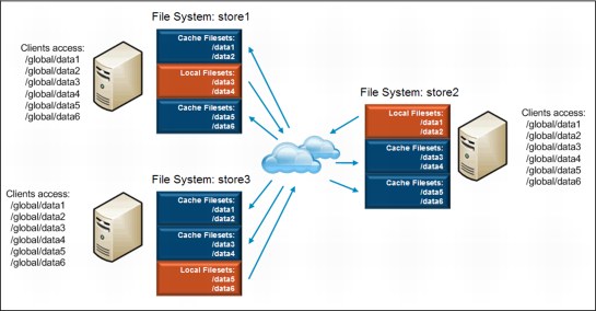
Figure 6-9 Global namespace
Solution for centralized data management for branch offices
In this scenario, assume that you have a geographically dispersed organization with offices of all different sizes. In the large offices, you have IT staff to perform data management tasks such as backups. In smaller offices, you need local systems to provide performance for the local user community, but the office is not large enough to warrant a complete backup infrastructure. You can use AFM in this case to provide a way to automatically move data back to the central site.
The AFM configuration contains a central site that has an NFS export for each remote site. Each remote site is configured as a single writer for that home. During a complete failure at the remote office, you can preinstall a new server at the central site by running a prefetch to fill the file system, then ship it to the remote office. When the new system is installed at the remote office, the data are there and are ready to continue serving files. In the meantime, the clients, if you like, can connect directly to the home for their data.
Figure 6-10 shows a central site where data are created, updated, and maintained. Branch sites can periodically prefetch by using a policy or pull on demand. Data is revalidated when accessed. Data are maintained at central location, and other sites in various locations pull data into cache and serve the data locally at that location.

Figure 6-10 Central and branch offices
Solution for data library with distributed compute
Sometimes as compute farms grow, it is impractical to scale up a full bandwidth network to support direct access to the library of data from each compute node. To address this challenge, AFM can be used to automatically move the data closer to the compute nodes that are doing the work.
In the example shown in Figure 6-11, the working set of data is relatively small, but the number of compute nodes is large. There are three GPFS compute clusters and one data library from the remote. When the job starts, the data that are needed for the job are prefetched from the library into each of the three cache clusters (Compute Cluster1, Compute Cluster2, Compute Cluster3). These cache clusters are within isolated InfiniBand networks that provide fast access to the copy of the data in the cache. This way, you can distribute the data close to the compute nodes automatically, even if the compute cluster are in different cities or countries.

Figure 6-11 Data library with distributed compute clusters
6.4.2 File Placement Optimizer (FPO)
The new FPO feature is available starting with GPFS 3.5.0.7, can be used only for Linux environments either on IBM System x or on IBM Power servers. FPO is designed for MapReduce workloads, present in the emerging class of big data applications. It aims to be an alternative for the Hadoop Distributed File System (HDFS) currently used in Hadoop MapReduce framework deployments.
IBM InfoSphere BigInsights 2.1, as a first example, integrates GPFS-FPO in its extended Hadoop MapReduce software stack:
How FPO works
All the cluster nodes are configured as NSD servers and clients to each other. Each node gets access to the local disk space of the other nodes. Such a setup is called shared nothing architecture or shared nothing cluster. Figure 6-12 presents a topology layout of the GPFS-FPO architecture.

Figure 6-12 GPFS-FPO topology layout
The configured local disk space of each node is aggregated by GPFS into a redundant shared file system. Traditional GPFS was able to provide this function, but only as a standard GPFS cluster file system. The GPFS-FPO extension additionally provides HDFS equivalent behavior, and even some enhancements through the following feature optimizations:
Locality awareness This is implemented by an extension of the traditional GPFS failure group notation from a simple integer number to a three-dimensional topology vector of three numbers (r, p, n) such as encoding rack, placement inside the rack, and node location information. Location awareness allows MapReduce tasks to be optimally scheduled on nodes where the data chunks are.
Chunks A chunk is a logical grouping of file system blocks allocated sequentially on a disk to be used as a single large block. Chunks are good for applications that demand high sequential bandwidth such as MapReduce tasks. By supporting both large and small block sizes in the same file system, GPFS is able to meet the needs of different types of applications.
Write affinity Allows applications to determine the placement of chunk replicas on different nodes to maximize performance for some special disk access patterns of the applications. A write affinity depth parameter indicates the approach for the striping and placement of chunk replicas in different failure groups and relative to the writer node. For example, when using three replicas, GPFS might place two of them in different racks to minimize chances of losing both. However, the third replica might be placed in the same rack with one of the first two, but in a different half. This way the network traffic between racks that is required to synchronize the replicas is reduced.
Pipeline replication Higher performance is achieved by using pipeline replication than is possible with single-source replication, allowing better network bandwidth utilization.
Distributed recovery Restripe and replication load is spread out this way over multiple nodes. That minimizes the effect of failures during ongoing computation.
New GPFS terms and commands options
When configuring a GPFS-FPO environment, specify related attributes for entities in the GPFS cluster at various levels: Cluster, file system, storage pool, file, failure group, disk, chunk, or block.
To help introduce the new features, the definitions for the storage pool and failure group notions are reviewed, and the format of the stanza file presented as already introduced by GPFS 3.5. Then, focus on the new FPO extensions that were introduced by GPFS 3.5.0.7.
For more information about these topics, see the product manuals at:
http://publib.boulder.ibm.com/infocenter/clresctr/vxrx/topic/com.ibm.cluster.gpfs.doc/gpfsbooks.html
For more information about the standard GPFS 3.4 with implementation examples for various scenarios, see Implementing the IBM General Parallel File System (GPFS) in a Cross-Platform Environment, SG24-7844, which is available at:
Storage pools and failure groups
A storage pool is a collection of disks that share a common set of administrative characteristics. Performance, locality, or reliability can be such characteristics. You can create tiers of storage by grouping, for example, SSD disks in a first storage pool, Fibre Channel disks in a second pool, and SATA disks in a third pool.
A failure group is a collection of disks that share a common single point of failure and can all become unavailable if a failure occurs. GPFS uses failure group information during data and metadata placement to ensure that two replicas of the same block are written on disks in different failure groups. For example, all local disks of a server node should be placed in the same failure group.
Specify both the storage pool and the failure groups when you prepare the physical disks to be used by GPFS.
The containing storage pool of a disk is specified as an attribute for the NSD. An NSD is just the cluster-wide name at the GPFS level for the physical disk. First define the disk as an NSD with the mmcrnsd command, then create a file system on a group of NSDs by using the mmcrfs command.
Stanza files
GPFS 3.5 extends the syntax for some of its commands with a stanza file option. Instead of a disk descriptor line for each considered physical disk, as specified in previous versions, now the file contains an NSD stanza. Example 6-1 shows an NSD stanza in a stanza file. The NSD stanza starts with the %nsd: stanza identifier, and continues with stanza clauses explained here by the preceding comments lines. The comments lines (#) are optional.
Example 6-1 NSD stanza example
%nsd:
nsd=gpfs001 # NSD name for the first disk device
# first disk device name on node n01
device=/dev/sdc
# NSD server node for this disk device
servers=n01
# storage pool for this disk
pool=dataPoolA
# failure group of this disk
failureGroup=2,1,0
The storage pool of the considered disk is specified as dataPoolA string value in the pool clause.
Extended failure group
The failure group clause of a disk can be specified not only as a single number such as in standard GPFS, but also as a vector of up to three comma-separated integer numbers. The line at the end of previous Example 6-1 specifies the failure group for the disk /dev/sdc, having a vector value of 2,1,0.
The vector specifies topology information that is used later by GPFS when making data placement decisions. This topology vector format allows the user to specify the location of each local disk in a node within a rack with three coordinate numbers that represent, in order:
•The rack that contains the node with the involved disk installed
•A position within the rack for the node that contains the involved disk
•The node in which the disk is located
Example 6-1 shows the topology vector 2,1,0 that identifies rack 2, bottom half, and first node.
When considering two disks for striping or replica placement purposes, it is important to consider the following factors:
•Disks that differ in the first of the three numbers are farthest apart (in different racks).
•Disks that have the same first number but differ in the second number are closer (in the same rack, but in different halves).
•Disks that differ only in the third number are in different nodes in the same half of the same rack.
•Only disks that have all three numbers in common are in the same node.
The default value for the failure group clause is -1, which indicates that the disk has no point of failure in common with any other disk.
The pool and failure group clauses are ignored by the mmcrnsd command, and are passed unchanged to the generated output file to be used later by the mmcrfs command.
Pool stanza
GPFS 3.5.0.7 extends the functionality for the storage pool object and adds a so-called pool stanza to pass FPO-related attributes to the mmcrfs or mmadddisk commands. A pool stanza must match the following format:
%pool:
pool=StoragePoolName
blockSize=BlockSize
usage={dataOnly | metadataOnly | dataAndMetadata}
layoutMap={scatter | cluster}
allowWriteAffinity={yes | no}
writeAffinityDepth={0 | 1}
blockGroupFactor=BlockGroupFactor
Block group factor
The new block group factor attribute allows GPFS to specify the chunk size. Chunk size is how many successive file system blocks to be allocated on disk for a chunk. It can be specified on a storage pool basis by a blockGroupFactor clause in a storage pool stanza as shown in the syntax above. This can also be specified at file level, by using by the --block-group-factor argument of the mmchattr command. The range of the block group factor is from 1 to 1024. The default value is 1. For example, with a 1 MB file system block size and block group factor of 128, you get an effective large block size of 128 MB.
Write affinity
The allowWriteAffinity clause indicates whether the storage pool has the FPO feature enabled or not. Disks in an FPO-enabled storage pool can be configured in extended failure groups that are specified with topology vectors.
The writeAffinityDepth parameter specifies the allocation policy used by the node writing the data. A write affinity depth of 0 indicates that each replica is to be striped across the disks in a cyclical fashion. There is the restriction that no two disks are in the same failure group. A write affinity depth of 1 indicates that the first copy is written to the writer node, unless a write affinity failure group is specified by using the write-affinity-failure-group option of the mmchattr command. For the second replica, it is written to a different rack. The third copy is written to the same rack as the second copy, but on a different half (which can be composed of several nodes). A write affinity depth of 2 indicates that the first copy is written to the writer node. The second copy is written to the same rack as the first copy, but on a different bottom half (which can be composed of several nodes). The target node is determined by a hash value on the file set ID of the file, or it is chosen randomly if the file does not belong to any file set. The third copy is striped across the disks in a cyclical fashion with the restriction that no two disks are in the same failure group.
|
Note: Write affinity depth of 2 is supported starting from 3.5.0.11(3.5 TL3)
|
Write affinity failure group
Write affinity failure group is a policy that can be used by an application to control the layout of a file to optimize its specific data access patterns. The write affinity failure group can be used to decide the range of nodes where the chunk replicas of a particular file are allocated. You specify the write affinity failure group for a file through the write-affinity-failure-group option of the mmchattr command. The value of this option is a semicolon-separated string of one, two, or three failure groups in the following format:
FailureGroup1[;FailureGroup2[;FailureGroup3]]
Each failure group is represented as a comma-separated string that identifies the rack (or range of racks), location (or range of locations), and node (or range of nodes) of the failure group in the following format:
Rack1{:Rack2{:...{:Rackx}}};Location1{:Location2{:...{:Locationx}}};ExtLg1{:ExtLg2{:...{:ExtLgx}}}
For example, the attribute 1,1,1:2;2,1,1:2;2,0,3:4 indicates the following locations:
•The first replica is on rack 1, rack location 1, nodes 1 or 2
•The second replica is on rack 2, rack location 1, nodes 1 or 2
•The third replica is on rack 2, rack location 0, nodes 3 or 4
If any part of the field is missing, it is interpreted as 0. For example, the following settings are interpreted the same way:
2
2,0
2,0,0
Wildcard characters (*) are supported in these fields. The default policy is a null specification, which indicates that each replica is to be wide striped over all the disks in a cyclical fashion such that no two replicas are in the same failure group. Example 6-2 shows how to specify the write affinity failure group for a file.
Example 6-2 Specifying a write affinity failure group for a file
mmchattr --write-affinity-failure-group="4,0,0;8,0,1;8,0,2" /gpfs1/file1
mmlsattr -L /gpfs1/file1
file name: /gpfs1/file1
metadata replication: 3 max 3
data replication: 3 max 3
immutable: no
appendOnly: no
flags:
storage pool name: system
File set name: root
snapshot name:
Write Affinity Depth Failure Group(FG) Map for copy:1 4,0,0
Write Affinity Depth Failure Group(FG) Map for copy:2 8,0,1
Write Affinity Depth Failure Group(FG) Map for copy:3 8,0,2
creation time: Wed May 15 11:40:31 2013
Windows attributes: ARCHIVE
Recovery from disk failure
Automatic recovery from disk failure is activated by the cluster configuration attribute:
mmchconfig restripeOnDiskFailure=yes -i
If a disk becomes unavailable, the recovery procedure first tries to restart the disk. If this fails, the disk is suspended and its blocks are re-created on other disks from peer replicas.
When a node joins the cluster, all its local NSDs are checked. If they are in a down state, an attempt is made to restart them.
Two parameters can be used for fine-tuning the recovery process:
mmchconfig metadataDiskWaitTimeForRecovery=seconds
mmchconfig dataDiskWaitTimeForRecovery=seconds
dataDiskWaitTimeForRecovery specifies a time, in seconds, starting from the disk failure, during which the recovery of dataOnly disks waits for the disk subsystem to try to make the disk available again. If the disk remains unavailable, it is suspended and its blocks are re-created on other disks from peer replicas. If more than one failure group is affected, the recovery actions start immediately. Similar actions are run if disks in the system storage pool become unavailable. However, the timeout attribute in this case is metadataDiskWaitTimeForRecovery.
The default value for dataDiskWaitTimeForRecovery is 600 seconds, whereas metadataDiskWaitTimeForRecovery defaults to 300 seconds.
The recovery actions are asynchronous, and GPFS continues its processing while the recovery attempts occur. The results from the recovery actions and any encountered errors are recorded in the GPFS logs.
GPFS-FPO cluster creation considerations
This is not intended to be a step by step procedure on how to install and configure a GPFS-FPO cluster from scratch. The procedure is similar to setting up and configuring a traditional GPFS cluster, so follow the steps in “3.2.4 Setting up and configuring a three-node cluster” in Implementing the IBM General Parallel File System (GPFS) in a Cross-Platform Environment, SG24-7844. This section only describes the FPO-related steps specific to a shared nothing cluster architecture.
Installing GPFS on the cluster nodes
Complete the three initial steps to install GPFS binaries on the Linux nodes: Preparing the environment, installing the GPFS software, and building the GPFS portability layer. For more information, see “Chapter 5. Installing GPFS on Linux nodes” of the Concepts, Planning, and Installation Guide for GPFS release 3.5.0.7, GA76-0413-07.
In a Technical Computing cloud environment, these installation steps are integrated into the software provisioning component. For example, in a PCM-AE-based cloud environment, the GPFS installation steps can be integrated within a bare-metal Linux and GPFS cluster definition. Or inside a more comprehensive big data ready software stack composed of a supported Linux distribution, GPFS-FPO as alternative to HDFS file system, and an IBM InfoSphere BigInsights release that is supported with the GPFS-FPO version.
Activating the FPO features
Assume that a GPFS cluster has already been created at the node level with the mmcrcluster command, and validated with the mmlscluster command. The GPFS-FPO license must now be activated:
mmchlicense fpo [--accept] -N {Node[,Node...] | NodeFile | NodeClass}
Now the cluster can be started up by using the following commands:
mmlslicense -L
mmstartup -a
mmgetstate -a
Some configuration attributes must be set at cluster level to use FPO features:
mmchconfig readReplicaPolicy=local
mmlsconfig
Disk recovery features can also be activated at this moment:
mmchconfig restripeOnDiskFailure=yes -i
mmlsconfig
Configuring NSDs, failure groups, and storage pools
For each physical disk to be used by the cluster, you must create an NSD stanza in the stanza file. You can find details about the stanza file preparation in “Pool stanza” on page 133. Then, use this file as input for the mmcrnsd command to configure the cluster NSDs:
mmcrnsd -F StanzaFile
mmlsnsd
Each storage pool to be created must have a pool stanza specified in the stanza file. For FPO, you must create a storage pool with FPO property enabled by specifying layoutMap=cluster and allowWriteAffinity=yes. The pool stanza information is ignored by the mmcrnsd command, but is used when you further pass the file as input to the mmcrfs command:
mmcrfs Device -F StanzaFile OtherOptions
mmlsfs Device
The maximum supported number of data and metadata replicas is three for GPFS 3.5.0.7 and later, and two for older versions.
Licensing changes
Starting with GPFS 3.5.0.7, the GPFS licensing for Linux hosts changes to a Client/Server/FPO model. The GPFS FPO license is now available for GPFS on Linux along with the other two from previous versions: GPFS server license and GPFS client license. This new license allows the node to run NSD servers and to share GPFS data with partner nodes in the GPFS cluster. But the partner nodes must be properly configured with either a GPFS FPO or a GPFS server license. The GPFS FPO license does not allow sharing data with nodes that have a GPFS client license or with non-GPFS nodes.
The announcement letter for the extension of GPFS 3.5 for Linux with the FPO feature provides licensing, ordering, and pricing information. It covers both traditional and new FPO-based GPFS configurations, and is available at:
A comprehensive list of frequently asked questions and their answers, addressing FPO among other topics, is available at:
Current limitations
These restrictions apply to the FPO feature at the GPFS 3.5.0.7 level:
•Storage pool attributes are set at creation time and cannot be changed later. The system storage pool cannot be FPO-enabled and have the metadataOnly usage attribute.
•When adding a disk in an FPO pool, you must specify an explicit failure group ID for this disk. All disks in an FPO pool that share an NSD server must belong to the same failure group. Only one NSD server can share the disks in an FPO pool. If one storage pool of a file system is FPO-enabled, all the other storage pools in that file system must be FPO-enabled as well.
•Nodes running the FPO feature cannot coexist with nodes that run GPFS 3.4 or earlier.
•The architectural limits allow FPO clusters to be scaled at thousands of nodes. GPFS 3.5.0.7 FPO feature tested limit is 64 nodes. Contact [email protected] if you plan to deploy a larger FPO cluster.
•All FPO pools must have the same blockSize, blockGroupFactor, and writeAffinityDepth properties.
•Disks that are shared among multiple nodes are not supported in an FPO file system.
•An FPO-enabled file system does not support the AFM function.
•FPO is not supported on the Debian distribution.
Comparison with HDFS
GPFS-FPO has all the ingredients to provide enterprise-grade distributed file system space for workloads in Hadoop MapReduce big data environments.
Compared with Hadoop, HDFS GPFS-FPO comes with the enterprise class characteristics of the regular GPFS: Security, high availability, snapshots, back up and restore, policy-driven tiered storage management and archiving, asynchronous caching, and replication.
Derived from the intrinsic design of its decentralized file and metadata servers, GPFS operates as a highly available cluster file system with rapid recovery from failures. Also, metadata processing is distributed over multiple nodes, avoiding the bottlenecks of a centralized approach. For Hadoop HDFS in the stable release series, 1.0.x and 0.20.x, the name-node acts as a dedicated metadata server, and is a single point of failure. This implies extra sizing and reliability precautions when choosing the hosting physical machine for the namenode. The 2.0.x release series of Hadoop adds support for high availability, but this cannot be considered yet for production environments as they are still in alpha or beta stages:
Also, GPFS follows POSIX semantics, which makes it easier to use and manage the files. Any application can read and write them directly from and to the GPFS file system. There is no need to copy the files between the shared and local file systems when applications that are not aware of HDFS must access the data. Also, disk space savings occurs by avoiding this kind of data duplication.
Because both system block size and larger chunk size are supported, small and large files can be efficiently stored and accessed simultaneously in the same file system. There is no penalty in using the appropriate block size, either larger or smaller, by various applications with different data access patterns, which can now share disk space.
..................Content has been hidden....................
You can't read the all page of ebook, please click here login for view all page.