Pricing Collateralized Debt Obligations—The Basics

The CDS discussed above transfers the credit risk of a single entity from the protection buyer to the protection seller for a contracted period. Where protection buyers seek to securitize large portfolios of default risk prone loans, or even CDSs, the collateralized debt obligations (CDO) is used.

How is a loan portfolio different from a single loan? We have seen above that the individual firms (in a loan portfolio) could default, leading to losses in the portfolio value. This risk can be assessed by estimating the PD for each firm and the LGD (1 – RR). Additionally, the degree of dependence in the portfolio between firms’ default probability, known as ‘default correlation’, has an impact on the timing of firms’ default, and, therefore, on the portfolio loss.

Understanding the CDO We have seen in the previous chapter that a CDO, like securitization, is a way of creating securities with differing risk characteristics from a portfolio of debt instruments.

However in a CDO, the portfolio comprises of heterogeneous instruments, such as senior secured bank loans, CDSs or high yield bonds (in securitization, it is typically a homogeneous pool of, say, home loans, auto loans, etc.). The basic structure of a CDO is as given in Figure 9.14.

Bank A, owner of a loan portfolio, wants to protect itself against the possible losses in the portfolio, but it does not want to ‘sell’ the portfolio. One way is to buy CDS for each borrower/firm in the loan portfolio, but that would be quite expensive. Further, individual CDS contracts do not protect against correlated defaults.

Bank A decides to buy protection through a CDO. In a typical CDO, the portfolio’s risk is ‘sliced’ into ‘tranches’ (‘tranche’ in French, means ‘slice’ and, in simple terms, every tranche is akin to tradable commercial paper) of increasing seniority and default risk of the underlying pool of loans (or CDSs).

Thus, each tranche in a CDO shows the priority of receiving payments from the underlying pool of assets, and also bearing the default risk. Each tranche is sold separately to investors according to their risk preferences, for a fee.

Cash flows are the critical link between the asset and liability sides of the CDO transaction. The asset side of the CDO is the underlying portfolio of reference assets—loans (or CDSs). The liabilities side comprises the securities issued by an issuer, which is typically a special purpose vehicle (SPV) that is a separate company or trust specially created for the transaction by the owner of the pool of assets. The SPV is created to insulate potential investors from the risk of failure of the CDO originator itself, say a bank.

Bank A, the originator of the CDO, sells the selected portfolio of assets whose credit risk is to be transferred, to the SPV, which in turn issues structured notes in the market backed by the portfolio of assets.

Let us now understand Figure 9.14. The first tranche (called the ‘equity tranche’) holds 5 per cent of the total notional loan principal, and absorbs all credit losses from the portfolio (during the life of the CDO) until the losses aggregate to 5 per cent of the notional principal. Hence the equity tranche is also called the ‘first loss tranche’, if the losses exceed 5 percent; the second tranche, which has 10 per cent of the loan principal, absorbs losses up to a maximum of 15 per cent (cumulatively). The third tranche holds 15 per cent of the principal and absorbs losses over 15 per cent up to a maximum of 30 per cent of the principal. The fourth tranche holds the bulk of the loan principal, 70 per cent, and absorbs all losses exceeding 30 per cent of the principal.

 

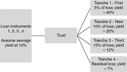
Now look at the yields (rate of interest paid) to the respective tranche holders. These rates are paid on the notional principal remaining in each tranche after the losses have been paid. Assume that tranche 1 suffers a loss of 1 per cent. The tranche holders, who were paid 40 per cent in case of no default, would now lose 20 per cent (1/5) of their investment, and would earn only on the remaining 80 per cent of their investment. Since they assume the first loss, taking the maximum risk, they are called the ‘equity tranche holders’. If the default loss were to rise to 3 per cent, this tranche would lose up to 60 per cent of the notional principal. Compare this with tranche 4. Defaults on the portfolio must exceed 30 per cent if this tranche is to suffer losses. Hence, this tranche is usually given the top rating (say AAA) by rating agencies. Since this is relatively safe investment, the tranche earns less for its holders. It is usual for Bank A, the originator of the CDO, to retain the equity tranche. The remaining tranches are sold in the market.

The transaction in the above example is termed ‘cash CDO’.

Typically, four broad types of CDOs are recognized—cash flow CDOs, market value CDOs, managed CDOs and static CDOs. The attributes of a specific CDO, such as MTM, rules related to trading of the underlying securities, etc., are determined by the type of CDO. For example, in a cash flow CDO, payments to investors are in the form of interest earnings and principal repayments from the underlying assets. Erosion in the underlying asset values would not usually have an impact on the cash flows to the investors in the CDO, unless the erosion is accompanied by a credit event. In this case, the interest/principal payments cease to flow from the asset originators to the SPV, leading to lower cash flow for the CDO investors. In the case of the market value CDO, changes in the MTM value are passed on to the CDO investors through the SPV.⁹⁹ In a managed CDO, the CDO manager actively trades the securities in the pool, with performance being monitored by the investors. In contrast, the static CDO’s portfolio is determined upfront and does not change over time.

If the portfolio of loans in the example is replaced by a portfolio of CDSs, the CDO is termed ‘synthetic CDO’.

Cash inflows to the synthetic CDO are the underlying CDS premiums, and cash outflows are losses consequent to credit events related to the underlying assets. Each tranche in a synthetic CDO has a specified upper and lower ‘detachment’ (U) and ‘attachment’ (L) point. Defaults affect the tranche according to the seniority of the tranche in the capital structure. The buyer of the tranche with attachment point L and detachment point U will bear all losses in the portfolio value in excess of L and up to U per cent of initial value of the portfolio. Table 9.13 presents the typical tranching done in the iTraxx index (Please see Box 9.10 for an introduction to credit indices).

 

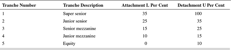
Assume that the above CDO experiences a 12 per cent loss of its initial value. This implies that the equity tranche holders will bear up to 10 per cent of the loss while the junior mezzanine holders would bear the remaining 2 per cent. The holders of more senior tranches (senior mezzanine, junior senior, super senior) will not suffer any loss. The super senior suffers only if the total collateral portfolio loss exceeds 35 per cent of its notional value.

Hence, it can be seen that CDO tranching enables holders of the respective tranches to limit their loss exposure to (U – L) per cent of the initial portfolio value.

For example,¹⁰¹ assume a hypothetical CDS index comprises of 100 names with equal weight (1/100) for each name. The tranches are indicated in the market as follows: 0–5, 5–10, 10–15, 15–22, 22–100. In other words, the 10–15 tranche has an attachment point L of 10 and a detachment point U of 15 and so on. We assume a specific investor has bought protection on the 0–5 per cent tranche with a notional principal of ₹10 crore. If one name out of the 100 defaults, and recovery is set at 65 per cent, the LGD is 35 per cent. In such a case the payout from the protection seller would be calculated using the formula—(notional principal × LGD × weighting)/tranche size, i.e., a payout of ₹70,000. Once the payout happens, the 025 tranche is recalculated to reflect the reduced notional principal. Hence 4.65 per cent (5 – 0.35 LGD) of the notional principal remains, which implies that the new detachment point should reflect that only 99 names now remain in the CDO. The new detachment point has to be now adjusted for the remaining names in the Index. It is to be noted that the original principal of the other tranches are not impacted due to this change, but have less protection against further losses.

The same concept can be used for determining the number of credit events at which the equity tranche stops covering losses, and the next tranche starts losing. The loss level in any given tranche depends on two random variables—the number of credit events in the entire portfolio and the related LGD. Assuming the LGD of 35 per cent in the previous paragraph applies to all defaulted firms in the portfolio (in reality LGD for each asset may be uncertain), the scenario under which the equity holders lose their entire notional principal (i.e., when the equity tranche gets fully written down to zero) will be given by the equation n number of defaults × ₹10 lakh per name notional × 35 per cent loss rate = 5 per cent equity tranche width × ₹10 crore million total portfolio notional.

Solving for n yields 14—the number of defaults for the equity tranche to be written down to zero. This means that the portfolio would have lost ₹50 lakh, at which point the equity tranche would be fully written down to zero. The next tranche, say, the junior mezzanine, would start losing from the 15th default onwards, and so on.

Pricing the CDO The concept of ‘default correlation’ is important to determine the pricing of a tranched CDO, such as tranched iTraxx.

For any two given firms, their default correlation approximates to a measure of the correlation between the times at which they default. In other words, two reference assets or firms which are highly correlated (correlation close to 1) are likely to behave similarly—either defaulting or not defaulting, together. This implies that a portfolio with several reference assets, who bear a high default correlation with one another, will have higher probabilities of both higher and lower loss rates. Consequently, the emanating loss distribution is likely to have fatter tails.

As default correlation increases in a portfolio, it is easy to understand why the cash flows from the underlying asset pool of loans or CDS would exhibit higher volatility. As volatility increases, the market value of the equity tranche (the highest risk bearing tranche) increases (and the spread decreases). On the other hand, since increased volatility (risk) is not favoured by the senior most tranche, the market value declines with an increase in default correlation, leading to higher spreads. The mezzanine and other tranches in between these two can have exposures to correlation in either direction, depending on the degree of volatility.

The basic methodology is to average the discounted cash flows to a particular tranche over several independently simulated scenarios. This implies that cash flows for each underlying single name CDS in the CDO have to be simulated, with correlation in the default times of the various underlying firms as well. The widely used industry methodology for the correlated default time simulation is the ‘Gaussian copula’ (in Statistics, ‘copula’ is used to couple the behaviour of two or more variables—however, a discussion on this is outside the scope of this book).¹⁰²

Box 9.10 introduces credit indices developed in credit derivative markets.

SECTION VII

CREDIT RISK MEASUREMENT AFTER THE FINANCIAL CRISIS

The Financial Crisis—An Overview and Analysis¹⁰³

When some of the world’s largest banks folded up quietly overnight in 2007–2008, afflicted by the ‘subprime crisis’, shaking up powerful economies, leaving stock markets and investors in a state of panic, taking centre stage in the crisis were the ‘villains’—structured products and the credit derivative.

The subprime crisis that began in mid 2007 is widely regarded as the first financial crisis in the age of mass securitization. It has unleashed a flurry of daunting questions on the very foundations of securitized finance and structured products. Just about everything related to the credit market is being questioned—is it right to originate and distribute? Is Basel II (to be discussed in a later chapter) adequate to control credit risks and ensure adequacy of bank capital? With its reliance on internal models and external credit rating agencies, can the credit risk be wished away by merely dispensing with complex derivatives? Is ‘financial engineering’ a dirty word?—and the debate goes on.

Funds and banks around the world purchased bonds or the risk related to bonds, backed by home loans, often bundled into CDOs. These CDOs were backed by pools of mortgages or other income-producing assets and considered essentially ‘bond like’ in that they offered investors a steady stream of returns. Investors found these securities attractive as they offered higher returns at a time when traditional fixed income or debt-related products were yielding lower returns. Investors also viewed these structured products to be quite ‘risk free’, when they were certified to be so by the top rating agencies of the world. The ability of ‘structured finance’ to repackage risks and create ‘safe’, tradable assets from risky, illiquid collateral was the reason for the meteoric increase in the issue of structured securities.

However, as low interest rates in many parts of the world fuelled a lending boom to less than creditworthy borrowers, banks looked for new avenues to package and sell these loans, so that they could get liquidity to lend more. By selling off risky loans, banks could maintain less regulatory capital commensurate with the risk. Hence banks and other financial institutions pooled these asset-backed securities into new pools, dividing them up and issuing securities against them, thus creating CDOs. The concept caught on pretty fast, with new combinations that were further and further removed from the original underlying asset. Such innovations included CDOs of CDOs or CDO-squared and even CDO-cubed.

According to J. P. Morgan, there are about $1.5 trillion in CDO, referring to those made up of bonds backed by subprime mortgages, slightly safer mortgages and commercial mortgage-backed securities.

Then what went wrong?

At the core of the crisis has been the housing boom in the United States since the beginning of the decade. Low interest rates meant home buyers could take larger loans, giving rise to a housing bubble marked by unrealistic optimism and a failure to consider the downside, since it was assumed that all foreseeable downside was taken care of while designing the securitized products. The cracks began showing in 2006, when subprime borrowers increasingly defaulted on monthly payments due to annual interest rate resets on their floating rate loans. Fears of recession caused bloated housing prices to dip alarmingly, and in 2007, prices of securities based on subprime loans were in free fall as investors feared that they would not get the promised payments from the structured securities. Lenders became wary and showed reluctance to lend.

With the underlying assets—the subprime mortgages—fast losing value, dangerous levels of leverage were revealed in the packaged securities, leading to the discovery that the ‘safe’ CDOs and other securities were actually far riskier than originally envisaged. As the complexity of these products increased, so did their opaqueness. The extent of losses that they have generated has surprised not only investors, but also the funds and bankers themselves. This was when weaknesses in the system were laid bare, including ratings that did not accurately reflect risk and faulty assumptions on how diversified pools would act on multiple layers of leverage.

The innovation in structured products was assisted by the rise of credit derivatives—especially CDSs. CDSs became staggeringly popular over the last few years throughout the developed world. CDSs resemble an insurance policy to the extent that they can be used by debt owners to hedge, or insure against a default on a debt. However, because there is no requirement to actually hold any asset or suffer a loss, CDSs could also be used for speculative purposes.

Thus, credit derivatives allowed banks to hedge their exposure to the subprime loans they had made, and also freed up capital—since they did not have to reserve capital for potential losses. The banks partnered with hedge funds—lightly regulated pools of capital with high fees—looking for better returns. Insurance companies and pension funds also sought the higher yields as interest rates hit historically low rates.

Annexure I presents a case study in the form of a brief chronology of events leading to the crisis that hit the United States and Europe.

Are structured products and credit derivatives really the villains of the high drama in the financial world? Who is responsible for the mammoth fiasco—Basel II, the rating agencies, the regulators or the banks themselves?

One possible inference is that the benefits of financial structuring and risk management are small compared to the huge costs they impose on financial stability and the reputation of banks. An alternative, therefore, is to return to ‘good, old-fashioned banking’ where banks create loans and hold them on their balance sheets and do not synthetically pool, package and distribute them.

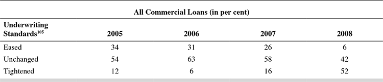
Another argument advanced against credit risk transfer mechanisms is that they create the problem of ‘moral hazard’. The originators of loans do not assess the credit quality with the same rigor that they would exercise were they to hold them on their balance sheets. This allegation seems to be true in the light of the findings of the 2008 and earlier surveys of credit underwriting practices in the United States.¹⁰⁴ The findings show that credit appraisal and delivery standards had in fact declined over the previous periods and banks have begun exercising more prudence in granting credit post the credit crisis. Table 9.14 summarizes the changes.

 

Basel II has also been squarely blamed for the incentive for banks to take risky assets off their balance sheet, or simply transfer the risk to willing sellers of protection—to comply with capital requirements. Theoretically, originators of loans can assume that assets or risks are off their balance sheet when they distribute them. Hence, the need to maintain capital on these assets is obviated. But for reputation, the originators may feel compelled to repurchase securities sold earlier. Then the assets come right back on the balance sheet—and when this would happen cannot be determined. For instance, Citigroup was seen to act responsibly when it included put options on CDOs backed by subprime mortgages that it sold to customers. The ‘puts’ gave the buyers the right to sell the securities back to the originator in case of financing problems. This contingency was not accounted for in the bank’s balance sheet.

Sophisticated financial models of asset portfolios have been built and used by the banking system and these have now come under the scanner. Were the financial models flawed or was there too much reliance on the results that they threw up? For example, Northern Rock, one of the biggest casualties of the UK, had reportedly carried out extensive stress testing as stipulated by the UK Financial Services Authority only in the first half of 2007 and the results sounded no alarm. Evidently, the probability that all the bank’s funding sources could dry up simultaneously was not one of the scenarios tested—since this looked highly improbable at that time!

The leading rating agencies of the world—S&P, Moody’s, Fitch—have all drawn huge flak for their ‘failure’ to distinguish the riskiness of different securities. They have been accused of being too generous with their AAA ratings, and worse still, overlooking the potential downfall of the market as the underlying mortgage assets deteriorated in value. The worst cut of all—they reacted with wholesale downgrades when the market collapsed. The possible conflicts of interest arising from rating agencies being paid by the issuers and the same agencies offering advisory services to the issuers are also areas drawing criticism.

And there could be other reasons too—Was it the structured investment vehicles (SIVs, similar to special purpose vehicles/entities (SPVs) or (SPEs) and other mechanisms that used short-term bank funding to invest in long-term derivatives, or was it their opaqueness, or was it the lack of proper regulation?

The Way Forward There are two alternatives before banks.

They return to ‘good, old-fashioned banking’, where banks originate and hold the assets till they are liquidated. But this option ignores economic realities. Deregulation has already come to stay, and structured products and risk management are inexorably linked with the broader deregulation of the financial markets and financial technology, backed by the dramatic leap forward of information technology and communication. Even if we turn the clock back and launch the era of strict and restrictive regulation, the advances made in communication and technology would make it possible for banks to move risks and assets offshore, and securitization would take a different form.

The second alternative is to recognize the real benefits of securitization and financial innovation—after all, these innovations have shown us methods of packaging and redistributing risk, transforming illiquid assets on bank balance sheets to tradable ones with attractive income streams; they have shown banks how to reduce holding costly capital to absorb the credit risk; they have given liquidity to the system and lowered funding costs.

Innovation has its costs too—as the present crisis has shown. But this is a necessary though unwelcome cost of learning. Pioneering efforts in any industry have always run into rough weather for lack of prior experience. The global turbulence is a heavy price to pay for innovation, but central banks and governments have acted swiftly to soften the blow to the banking system and markets.

The present crisis can therefore be considered a maturity crisis of the credit market after the development of credit derivatives. At first glance, it looks like a massive failure of most used quantitative models of credit derivative pricing. However, we would have to remember here that there is a basic risk involved in lending money, and that this risk comes at a price, and credit derivatives have found a way to merely transfer this risk, but not to wish risk away! Probably, armed with a deeper understanding of the causality of the credit default process, deductive models with better and better predictive ability can take care of the changing environment.

The signals are now quite clear. The OCC Survey sums it up neatly. ‘While the competitive environment will inevitably cause changes in credit underwriting standards, banks need to have risk management and control processes to signal when standards veer away from safe and sound banking practices. Banks should underwrite credit based upon an expectation that the borrower can repay the loan, regardless of whether the loan is intended for portfolio or for distribution. As recent events have clearly shown, liquidity conditions in credit markets can change abruptly. Banks originating credit for distribution should maintain underwriting standards reasonably consistent with the standards for their own portfolio holdings.’¹⁰⁶

Current Developments and Regulatory Changes

In a bid to ensure the stability of the financial system, several regulatory and market-related changes are being introduced. One of the focus areas of these changes is credit derivatives. Even though public interest has turned towards the credit derivatives market only recently, the derivatives market has been focused on by regulators over the years. Regulatory attention is now most pronounced in the United States and Europe, where the crisis has taken its severest toll.¹⁰⁷

A major lesson of the crisis seemed to be insufficient regulatory oversight over CDS and other structured instruments. In its final report, the US Financial Crisis Inquiry Commission (FCIC 2011, p 50) noted that “key OTC derivative in the financial crisis was the Credit Default Swap”.

Some of the important international regulatory developments in the CDS markets are given below:

1. USA - The Dodd Frank Act (2010)¹⁰⁸

Deemed as one of the greatest regulatory overhauls of financial markets after the Glass Steagall Act almost eight decades earlier, the Dodd Frank Act contains at least three regulatory aspects that directly impact the CDS market. One, the Volcker Rule, which separates proprietary trading from commercial banking activities; two, the central clearing of CDS indices, and three, the gradual phasing out of uncleared single name CDS.

2. European Union - MIFID II and MIFIR (2014)¹⁰⁹

In October 2011, the European Commission adopted a legislative proposal for the revision of Markets in Financial Instruments Directive (MiFID) which took the form of a revised Directive and a new Regulation. After more than two years of vigorous debate, the Directive on Markets in Financial Instruments repealing the earlier Directive in 2004 and the Regulation on Markets in Financial Instruments, commonly referred to as MiFID II and MiFIR, were adopted by the European Parliament on 15 April 2014, by the Council of the European Union on 13 May 2014 and published in the EU Official Journal on 12 June 2014.

Building on the rules already in place, these new rules are designed to take into account developments in the trading environment since the implementation of MiFID in 2007 and, in light of the financial crisis, to improve the functioning of financial markets making them more efficient, resilient and transparent.

3. Basel III Regulations

The Basel regulations, which is being discussed in detail in Chapter 11, prescribe international standards for bank capital and associated risks, with a view to lending more stability to the global financial system.¹¹⁰

Basel 3 is currently being implemented, but there has been an almost constant review of various standards, which is being labelled widely as Basel 4. Currently, revisions are in place for market risk and counterparty risk, as well as securitization exposures. A notion of ‘liquidity horizons’ has been introduced. Valuation of illiquid positions such as CDS and Mortgage backed securities are also expected to be impacted.

The treatment of counterparty credit risk (CCP), the risk associated with derivatives has already been subject to substantial change under Basel 3 after the financial crisis.

A new credit valuation adjustment (CVA) volatility charge is being introduced by Basel 3. There are basically two ways to incorporate credit risk in valuing a derivative portfolio. One way is to discount expected cash flows of the financial asset, say a CDS, at a discount rate incorporating a credit risk adjustment. The other way is to apply a CVA. The CVA is the expected value or price of counterparty risk. The asset is valued at a risk free price (no credit risk) and a specific adjustment is made for counterparty risk. Basel 3 has introduced more stringent requirement for Internal Models Methodology (IMM) for determining capital requirements.

Some developments

Ironically, about two years after the Dodd Frank act was passed, the large trading loss sustained by J P Morgan in early 2012 once again focussed on CDS. Dubbed as the London Whale case, this event once again served to highlight ineffective risk management in CDS trading strategies. The call for more stringent CDS regulations grew louder.

In the second half of 2015, the CDS market faced another tough challenge. A $1.86 billion settlement in favour of the Los Angeles Country Employees Association was made. The defendants in the case included 12 major Wall Street banks, the CDS industry representative ISDA (International Swaps and Derivatives Association) and the CDS data provider Markit Group Ltd. The defendants were accused of obstructing efforts in making the transactions more transparent.

Deutsche bank, a major participant in the CDS market, closed their books for single name corporate CDS in October 2014. In May 2015, the world’s largest asset manager, Black Rock, called for a market wide effort to revive the single name CDS market.

Central clearing, an important requirement of Dodd-Frank, will have to cover most CDS. From February 2014, The CDS Index trades have to be traded on Swap Execution Facilities and centrally cleared. However, single name CDS are not part of the central clearing system, which could distort the CDS index market.

However, the BIS quarterly review of June 2017¹¹¹ notes that the share of outstanding CDS cleared through central counterparties (CCP) “jumped from 37% of notional amounts outstanding at end- June 2016 to 44% at end-December 2016. This movement represented the largest semiannual increase in the centrally cleared share since CCP data for CDS were first collected in 2010. The proportion of outstanding CDS contracts centrally cleared increased for single-name as well as multi-name instruments, although the proportion remained much higher for the latter: 54% compared with 36%. Multi-name products tend to be more standardised than singlename products and consequently more amenable to central clearing. Notably, the increase in the proportion was driven by a sharp decline in the uncleared segment of CDS markets. Whereas the notional amount cleared through CCPs was more or less unchanged in the second half of 2016, at $4.3 trillion, the notional amount for contracts between reporting dealers fell from $5.1 trillion to $3.7 trillion.”

However, it is noteworthy that the CDS market (outstanding notional size) had grown from less than $1 trillion in 2001, to over $60 trillion by 2007, when the financial crisis happened. The CDS market is currently at a fraction of its pre crisis levels.

SECTION VIII

A NOTE ON DATA ANALYTICS¹¹² AND BUSINESS SIMULATION

‘Analytics will define the difference between the losers and winners going forward,’—Tim McGuire, a McKinsey director.

By this time, you would have understood that behind effective risk management, and a successful model that aids risk management, lies a very important ingredient – Information. Valuable information, in turn, is embedded in data that is grouped and analyzed to yield information for decision making and management. Banks and firms now realize that data and its proper analysis can be used effectively to increase productivity, improve decision making, enhance risk management capabilities and thus gain competitive advantage. Experts call it the ‘big data’ revolution.

In the world of finance, we know that ‘information’ has value. However, voluminous and unstructured data or information that most banks and firms seem to have today cannot be managed or analyzed by traditional tools. For example, banks traditionally gather data for reporting purposes—to their head offices, to central banks, to the government, to the public and so on. However, today data signifies not only the traditional data, but also enormous amounts of data that converge from click stream sources from the web, social media, and videos. Banks’ back offices generate voice data. Data is generated through the ‘cloud’. (It is estimated that Google alone processes over 24000 terrabytes per day!). However, these unconventional information sources are not tabulated in typical rows and columns that one can read or interpret.

Banks, in particular, have access to enormous information—customer data, transaction details, performance data, credit information, and so on—from both internal and external sources.

So the first question is—what is the data that they want to use and for achieving what purpose? With the help of advanced technology, it is now easy to gather data and store it. But the challenge is to determine which data to use, the best source for the data, and how to put it together into an integrated form that can serve the objective across the bank.

Therefore, a key capability to utilize the information explosion for data analytics is to identify, integrate and manage diverse sources of data. Another key capability is to build or use the vast data in advanced analytics models that would realistically predict future trends and outcomes. Of course, the most important requirement is the capability of management to integrate the data analytics models into the firm’s functioning so that better decisions can be made. The latter capability presupposes the existence of a clear strategy for transforming the way the firm works through data analytics, and the use of the most appropriate technology infrastructure and human skills. All this implies that the approach to using analytics for optimal decision making should be integrated with the sourcing of the correct and appropriate data. Information is costly, and lack of vision in collecting data and wondering how to use the data would lead to loss of productivity and undermine the firm’s competitive ability.

Banks need data analytics in a big way for managing risks—be it credit risk, market risk, operational risks, liquidity risk, or the interplay of various risks on the financial system. While regulatory prescriptions for risk management are driving banks to ‘big data’ analytics, banks are using the data generated for internal management as well.

Banks can benefit from ‘big data’ in a big way. The following diagram illustrates.

Business Simulations: 5 Reasons Why Business Simulations Are Great Learning Tools¹¹³

1. Risk Free Learning

One of the very foundations of the ‘learning by doing’ concept of business games is the acceptance of failures, and the ability of deriving valuable learning from them. This very basic principle is what made Silicon Valley become the unique and striving start-up hub it is today, and it is most valuable skill for students to get a complete hands on before embarking on their journey as working adults. Business management simulations are the safer ways of helping the students first learn how to navigate the landscape of a real company, than losing out all their savings on a badly executed business idea or venture.

One of the key differentiators of business simulation games is that it acts as an excellent tool to practice real world business decision-making skills as everything happens in a risk free simulated learning environment. This encourages the students to try out different strategies, observe the results, monitor market fluctuations, then pivot their direction, all without real-life repercussions.

2. Multiplayer Environment

With the massive surge of multiplayer online games, most college students today prefer an environment where they could interact with other players in either a cooperative or competitive fashion. Business Games brings people together in virtual worlds, mirroring the phenomenon of increased internationalization and cross-border cooperation between businesses as well, a need of the hour.

In business simulation games students form the management teams of a virtual company that competes against other companies in the same market for a slice of the consumer pie. Today business simulation games with a fully web-based platform supported by an in-game messaging system, enables these teams from anywhere in the world to improve cross-campus cooperation and create exciting competitions between partner universities.

3. Interactive Game Play

Another major appeal of many games would be their real time feedback on decisions made. This feature just not only makes participants more engaging, but also helps them practice a number of different strategies in a short period of time and discover what works best or better.

Most Business Simulation Games employ a round-based system which gives the students an opportunity to strategize with their teammates before coming to any final decisions, and also enabling the instructors/facilitators to schedule and manage his/her course better. The dynamic aspect is prevalent however in the decision-making areas, where students can immediately see the effect of their choices once they start experimenting with the decisions.

4. Realistic Story Arc

Good stories always captivates human brains, in business as well as in games, story driven game plays are very successful in enticing large audiences.

In higher education stories have been encapsulated in case studies, which although take students through a particular segment of a company’s life, it happens in a non-interactive format. Business Simulations on the contrary enables the students to further immerse by actually becoming the protagonists of their company’s story, and determining its faith through decisions made in a volatile environment. This not only does give students a greater sense of purpose, but also make them think much more carefully about their actions when they don’t only exist in theory.

5. In-game Rewards

What would this entire experience be without any satisfying rewards? Just like in any traditional games, business simulations also do reward players in one or more ways, most notably would be the rankings on the leader board, and/or by a market leadership position with a great cumulative total on business profits, shareholder returns, etc.

But the most valuable rewards for students is ultimately help them improve on their business decision making skills, holistic thinking, teamwork, proactive pivoting, and problem solving skills, all of which will be retained substantially longer than by others, less active forms of learning.

CHAPTER SUMMARY

• Traditional methods such as the Altman’s Z score and other credit scoring models try to estimate the PD, rather than potential losses in the event of default (LGD). The traditional methods define a firm’s credit risk in the context of its ‘failure’—bankruptcy, liquidation or default. They ignore the possibility that the ‘credit quality’ of a loan or portfolio of loans could undergo a mere ‘upgrade’ or ‘downgrade’
• The credit risk of a single borrower/client is the basis of all risk modelling. In addition, credit risk models should also capture the ‘concentration risk’ arising out of portfolio diversification and correlations between assets in the portfolio. Typically, credit risk models are expected to generate (a) loss distributions for the default risk of a single borrower and (b) portfolio value distributions for migration (upgrades and downgrades of a borrower’s creditworthiness) and default risks.
• Credit risk models have a wide range of applications. They are prevalently used for the following:
  1. Assessing the ‘EL’ of a single borrower.
  2. Measuring the ‘economic capital’ of a financial institution
  3. Estimating credit concentration risk
  4. Optimizing the bank’s asset portfolio
  5. Pricing debt instruments based on the risk profile

  Credit risk models are valuable since they provide users and decision makers with insights that are not otherwise available or can be gathered only at a prohibitive cost.

• ‘Creditmetrics™’, the most well-known industry-sponsored credit migration model applies migration analysis to credit risk measurement. The model computes the full (1 year) forward distribution of values for a loan portfolio, where the changes in values are assumed to be due to credit migration alone, while interest rates are assumed to evolve in a deterministic manner. ‘Credit VaR’ is then derived as a percentile of the distribution corresponding to the desired confidence level.
• CPV is a ratings-based portfolio model used to define the relationship between macroeconomic cycles and credit risk in a bank’s portfolio. It is based on the observation that default and migration probabilities downgrade when the economy worsens, i.e., defaults increase, and the contrary happens when the economy strengthens. The model simulates joint conditional distribution of default and migration probabilities for non-IG borrowers whose default probabilities are more sensitive to credit cycles, which are assumed to follow business cycles closely, than those of highly rated borrowers in different industries and for each country, conditional on the value of macroeconomic factors.
• MKMV uses the option pricing framework in the VK model to obtain the market value of a firm’s assets and the related asset volatility. The default point term structure for various risk horizons is calculated empirically. MKMV combines market value of assets, asset volatility and default point term structure to calculate a DD term structure, which is then translated into a credit measure termed (EDF). The EDF is the PD for the risk horizon (1 year or more for publicly traded firms).
• Credit risk+ has been developed based on the actuarial approach by Credit Suisse financial products (CSFP). In this model, only default risk is modelled, not downgrade risk. The model makes no assumptions about the causes of default. Each borrower/counter party can assume only one of two ‘states’ at the end of the risk horizon,—‘default’ (0) or ‘no default’ (1). All the above models are commonly known as ‘structural models’.
• The other class of popular models is ‘reduced-form’ models. The key difference between structural and reduced-form models is in the ‘information’ available to model credit risk. While ‘defaults’ are specified ‘endogenously’ (the credit quality being determined by the assets and liabilities of the firm) in structural models, defaults are modelled exogenously from market data in the reduced-form approach. Another difference is in the treatment of RRs—structural models specify RRs based on the value of assets and liabilities within the firm, while reduced-form models look to the market to specify RRs. Reduced-form models are also called ‘intensity’ models. If information available to the modeller/bank is partial or incomplete, a structural model with default being a predictable ‘stopping time’ becomes a reduced-form model with default time being unpredictable.
• There are several methodologies used to price CDS spreads. The reduced-form models are also used for this purpose. The concept of ‘default correlation’ is important to determining the pricing of a tranched CDO, such as tranched iTraxx.
• 2001 saw the launch of synthetic credit indices by J.P. Morgan (JECI and Hydi), and Morgan Stanley (Synthetic Tracers). In 2003, these indices were merged under the name Trac-x. At around the same time, credit derivative indices were introduced by iBoxx. Further consolidation took place in 2004 when Trac-x and iBoxx combined to form the CDX in North America, and the iTraxx in Europe and Asia. Since November 2007, Markit owns the iTraxx, CDX, LevX and LCDX indices for derivatives, and iBoxx indices for cash bonds.
• The Credit Event Fixings have been developed by Creditex and Markit along with ISDA and major dealers in credit derivatives. The objective of credit fixings is to ensure a fair, efficient and transparent process for settlement of credit derivative trades following a corporate default. They are an integral part of ISDA’s CDS Index protocols.
• The subprime crisis that began in mid 2007 is widely regarded as the first financial crisis in the age of mass ‘securitization’. It has unleashed a flurry of daunting questions on the very foundations of securitized finance and structured products, as well as credit risk models and rating agencies.
• In a bid to ensure the stability of the financial system, several regulatory and market-related changes are being introduced. One of the focus areas of these changes is credit derivatives. Regulatory attention is now most pronounced in the United States and Europe, where the crisis has taken its severest toll.
• Banks and firms realize that data and its proper analysis can be used effectively to increase productivity, improve decision making, enhance risk management capabilities and thus gain competitive advantage. Experts call it the ‘big data’ revolution. Data analytics is transforming the way banks function.

TEST YOUR UNDERSTANDING

1. Rapid fire questions

   Answer ‘True’ or ‘False”

   1. Traditional credit scoring models try to estimate the probability of default of a borrower and the potential losses in the event of default.
   2. Expected loss for a credit portfolio is the product of probability of default, loss given default and exposure at default.
   3. Credit risk models can be used to price credit instruments based on the risk profile.
   4. Credit Value at Risk conforms to the normal distribution.
   5. Credit migration models use the option pricing theory for determining probability of default.
   6. Credit Metrics is an industry sponsored credit migration model.
   7. Credit Portfolio View (CPV) was developed by Mckinsey and co.
   8. In the MKMV model, Expected Default Frequency (EDF) is the probability of default.
   9. EDF measures are credit scores.
   10. Credit Risk + uses the actuarial approach to modelling PD.

   Check your score in Rapid fire questions

   1. False
   2. True
   3. True
   4. False
   5. False
   6. True
   7. True
   8. True
   9. False
   10. True
2. Fill in the blanks with appropriate words and expressions
   1. If a firm has a current EDF measure of 3%, it implies that the firm has a —————% probability of defaulting over the next ————— months.
   2. Reduced form models assume no explicit relationship between ————— and firm value.
   3. Reduced form models are also called ————— models.
   4. Default by the borrower is called a credit event in a ————— contract.
   5. Typically, four broad types of CDOs are recognized - ————— CDOs, ————— CDOs, ————— CDOs and ————— CDOs.
   6. When a CDO is built from a portfolio of CDS, it is termed a ————— CDO.
3. Expand the following abbreviations (in the context of this chapter)
   1. MiFID
   2. CVA
   3. CCP
   4. CDO
   5. DD
   6. EDF
   7. RR
   8. ISDA
4. Test your concepts and application
   1. Which of the following loans is most risky? Assume that other things are equal—the borrowers are rated the same, are from the same industry and have the same risk profile.
      1. ₹30 crore loan with 50 per cent LGD
      2. ₹10 crore loan with no collateral
      3. ₹40 crore loan with 40 per cent RR
      4. ₹40 crore loan with 40 per cent LGD
   2. Which of the following loans is likely to have the highest PD, other things being equal?
      1. The loan with the longest maturity
      2. The loan with the lowest LGD
      3. The loan whose value has the lowest volatility
      4. The loan whose borrower is assessed most creditworthy
   3. Which of the following is NOT used to estimate the PD of a firm in the KMV model?
      1. Book value of equity
      2. Market value of equity
      3. Book value of debt
      4. Price volatility
      5. Time to maturity of loan to the firm
   4. Using the KMV credit risk model, calculate the DD of a firm whose assets stand at ₹50 crore at current value, and whose liabilities are at ₹30 crore. Also assume the asset return volatility is 10, and the conditions of the Merton model are met.
   5. Which of the following is NOT TRUE of MKMV’s EDF?
      1. EDF measures are actual probabilities
      2. EDF measures are credit scores
      3. If a firm has a current EDF credit measure of 2 per cent, it implies that there is a 2 per cent probability of the firm defaulting over the next 1 year
      4. If there are 100 firms with an EDF of 4 per cent, we can expect, on an average, four firms to default over the next year
      5. A firm with 4 per cent EDF measure is 10 times more likely to default than a firm with 0.4 per cent EDF measure
   6. For a portfolio of risky assets, Credit Metrics uses the following to estimate default correlations.
      1. Correlation of changes in corporate bond yields
      2. No default correlations are assumed
      3. Correlation of changes in corporate bond defaults
      4. Correlation of equity returns
   7. In Illustration 9.3 (Credit Risk+), if in step 2, for the same bands and number of borrowers in each band, the expected number of defaults in each band doubles, what will be the effect on the EL in each band?
   8. A 5-year CDS requires semi annual payment at the rate of 60 bps per annum. The notional principal is ₹30 crore. A credit event occurs after 4 years and 5 months. If the RR is 40 per cent, and the CDS is settled in cash, list the cash flows and their timing for (a) the protection buyer and (b) the protection seller.
   9. What is the difference between (a) a plain vanilla CDS and a binary CDS, and (b) a plain vanilla CDS and a basket default swap?
   10. How would the CDS fee (spread) change in Illustration 9.5 if (other things remaining constant)
       1. The fee payments were made quarterly
       2. The fee payments were made semi annually
       3. The default occurred mid way during the year
       4. The RR was more than 50 per cent
       5. The RR was less than 50 per cent
       6. It is a binary CDS.
   11. Denote conditional default probability for a firm X as p per year, and the RR as R. The risk-free rate is 5 per cent per year. Default always occurs at the end of the year. The spread for a 5-year plain vanilla CDS is 120 bps and the spread for a similar 5-year binary CDS is 160 bps. What is the value of p and R?
   12. How would p and R in the above example change if defaults always occurred mid way through every year? Would you be able to draw any conclusion about the relationship between the spreads of a similar plain vanilla CDS and binary CDS?

TOPICS FOR FURTHER DISCUSSION

• For a hypothetical loan/loan portfolio, apply the credit risk models and compare the results.
• MKMV publishes on its Web site, case studies on calculating EDF for several firms. Take a sample of these firms and trace their credit ratings as awarded by the top credit rating companies to these firms. Are the results consistent?
• Should credit derivatives be continued as credit risk transfer mechanisms, in the light of their role in the current global financial crisis?
• What are CDO-squared and CDO-cubed and how are they valued?
• What are the various types of exotic CDOs and how are they priced?
• Are structured products like the CDS adding to or mitigating risk for the financial system? How effective have the new regulations been in risk management?

SELECT REFERENCES

1. Bluhm, Christian, Ludger Overbeck and Christoph Wagner (2003) An introduction to credit risk modelling. CRC Press LLC, USA, ISBN 1-58488-326-X.
2. Crouhy, M, Dan Galai and Robert Mark, (2000). ‘A Comparative Analysis of Current Credit Risk Models’, Journal of Banking and finance 24: 59–117.
3. Elizalde, Abel. (2005a) ‘Credit Risk Models I: Default Correlation in Intensity Models’, accessed at www.abelelizalde.com.
4. Elizalde, Abel. (2005b) ‘Credit Risk Models II: Structural Models’, accessed at www.abelelizalde.com.
5. Elizalde, Abel (2006), ‘Credit Risk Models III: Reconciliation Reduced-Structural Models’, CEMFI working paper 0607, accessed at www.cemfi.es
6. Gordy, Michael (2000), ‘A Comparative Anatomy of Credit Risk Models’, Journal of Banking and Finance 24: 119–149.
7. Hull, John, and Alan White (2008), ‘Dynamic Models of Portfolio Credit Risk: A Simplified Approach’, Journal of Derivatives 15, 4 (Summer): 9–28.
8. Jarrow, Robert A. and Stuart M. Turnbull (2000), ‘The Intersection of Market and Credit Risk’, Journal of Banking and Finance 24: 271–299.
9. Merton, Robert C. (1974), ‘On the Pricing of Corporate Debt: The Risk Structure of Interest Rates’, Journal of Finance 39: 449–470
10. Uwe, Wehrspohn. (2002), ‘Credit Risk Evaluation: Modelling–Analysis–Management’, accepted as a doctoral thesis at the faculty of economics at Heidelberg University, Germany, available in e-book-format at http://www.risk-and-evaluation.com.
11. http://www.defaultrisk.com
12. http://www.bis.org

ANNEXURE I

CASE STUDY-THE GLOBAL CREDIT CRISIS—A BRIEF CHRONOLOGY OF EVENTS IN 2007–08

This case study is presented as a chronology of events that led to the financial crisis of 2007-2008.

Months	2007	2008
January		A dismal dawn to the new year as bank losses continue to plague the market. Bear Stearns discloses subprime losses of $1.9 billion, leading to the exit of its CEO. Countrywide’s shares plumb new depths and Bank of America steps in to buy it for $4 billion. Citigroup has a further $18 billion of losses to report in its mortgage portfolio, while Investment banker Merrill Lynch projects $15 billion of subprime losses. French bank Societe Generale takes a hit of 4.9 billion euros due to unauthorized activities of rogue traders. Financial losses translate into job losses. Lehman Brothers retires from wholesale mortgage lending and announces 1,300 job cuts. United States estimates 35,000 job losses in residential construction and mortgage lending. Rating downgrades also happen simultaneously. In a first of its kind move, Fitch downgrades Ambac, the second largest monoline insurer. In spite of successive cuts in fed funds rate to stand at 3 per cent, World Bank says that world economic growth will slow in 2008.
February	US senate Banking committee holds first meeting on predatory lending in subprime sector after Ownit Mortgage Solutions filed for bankruptcy in December 2006. In the same month, HSBC loses over $10.5 billion, and the Head of HSBC US mortgage lending business is fired.	In an attempt to stem the rot, President Bush signs the Economic Stimulus Act of 2008. However, the downslide continues. UBS announces fourth quarter 2007 loss of CHF 12.4 billion ($12 billion). AIG, one of the largest insurers, announces fourth quarter 2007 losses of $5.3 billion due to more than $11 billion of losses on its CDS portfolio.
March	FDIC issues a cease and desist order against subprime lender Fremont Investment & Loan, which had been operating without adequate subprime mortgage loan underwriting criteria. The New York Attorney General announces investigation into subprime lending after lenders cut off credit lines to New Century Financial, a large subprime lender, and trading in its shares is sus pended, and Accredited Home Lenders decide to sell, at heavy discount, $2.7 billion of their subprime loans.	The delinquency rate on mortgages increases 87 bps to 5.82 per cent during fourth quarter 2007 over the same period previous year, according to MBA’s National Delinquency Survey. Reflecting this trend, Carlyle Capital, a highly leveraged fund (30 times) mostly invested in agency-backed RMBS, defaults on $17 billion of debt. A larger shock comes later in the month, when a near insolvent Investment bank Bear Stearns is bid for by JP Morgan Chase at $2 per share. JP Morgan raises its bid to $10 per share and agrees to indemnify the Federal Reserve Bank of New York against the first 1 billion of losses, based on the latter’s guarantee covering $30 billion of Bear Stearns assets, mostly mortgage-related,. To ease the situation further, The Federal Reserve Bank of New York announces TSLF, which lets primary dealers swap AAA-rated securities for Treasury securities. It also creates PDCF, to throw open the discount window to primary dealers and non-depository institutions. A further cut in the fed funds rate brings it to 2.25 per cent.
		The Federal Reserve, European Central Bank and Swiss National Bank also increase the size of their dollar swap lines to $30 billion and $6 billion, respectively.
April	New Century Financial, dealing in subprime loans, files for bankruptcy, while the National Association of Realtors announces a more than 8 per cent decline in existing home sales during a single month, the largest in 18 years	As losses continue, so does the scramble for funds by major banks. While Citigroup announces a further subprime loss of $12 billion, and UBS AG, the European bank hardest hit by the crisis announces further losses, Washington Mutual, one of the largest US mortgage originators, raises $7 billion from TPG, a private equity firm. National City Corp., a large regional US bank, seeks a $7 billion capital infusion from another private equity firm, Corsair Capital. And Royal Bank of Scotland announces that it will sell assets and approach investors to raise about £16 billion. Hedge funds rush in to make the most of the market tumble, by shorting the mortgage market, thus, worsening the situation. Fed funds rate is scaled down further to 2 per cent. IMF’s Global Financial Stability estimates total credit losses of $1 trillion, of which $510 billion will be borne by banks. According to the IMF, the crisis has spread beyond the subprime, and has affected other mortgage bonds, securitized car and student loans, leveraged lending backing private equity buyouts and credit derivatives.
May	As GMAC, the finance arm of General Motors, reports home loan losses of $1 billion and UBS closes its US subprime business, the first comprehensive plan to help homeowners avoid foreclosures is presented in the US Senate. Some banks enter a sell off mode to raise long-term funds even as UK mortgage lender Kensington agrees to a $561 million takeover offer from South African bank, Investec.	Cities and towns rarely go bankrupt. But the city council of Vallejo, California, files for bankruptcy since its declining housing-related tax revenues are not enough to pay for basic services. Reports of first quarter 2008 losses continue to come in. UBS AG announces CHF 11.5 billion ($11.1 billion) loss, while monoline insurer MBIA announces a $2.4 billion loss. Fannie Mae also discloses $2.2 billion losses, but says it planned to raise $6 billion in capital, after the regulator gives it the go ahead to expand its activities even while being involved in the credit squeeze. Citigroup plans a massive wind down of $400 billion of assets over the next 3 years, after raising $44 billion in capital through stock sales and private offerings to investment funds abroad.
June	CDO prices fall, and Bear Stearns is forced to prop up two of its hedge funds with a $3.2 billion injection. At around the same time, fearing a backlash of the developing crisis in the United States, the Bank of England reduces the overnight bank rate by 25 basis points to 5.5 percent.	S&P downgrades Morgan Stanley, Merril Lynch and Lehman brothers, the second, third and fourth largest investment banks in the United States, and announces a ‘negative’ outlook on all four largest investment banks, including Goldman Sachs. The rating agency also downgrades MBIA and Ambac, US’ large insurers. More and more banks in the United States announce dividend cuts and asset write downs. The UK’s share of woes increases as Bradford and Bingley, UK’s largest buy-to-let mortgage lender announces lower profits and sale of 23 per cent stake to US-based private equity firm, TPG.
July	As US housing prices plunge 20 per cent over the previous year, the three major credit rating agencies drastically lower their ratings of the subprime bonds, creating panic among investors. General Electric decides to sell WMC Mortgage, its subprime lending business. More serious, the two distressed Bear Stearns funds file for bankruptcy protection. As fear spreads, UK authorities take action against five brokers selling subprime mortgages	Freddie Mac and Fannie Mae fall by over 60 per cent over the year, on concerns that the capital they raised since December may not be sufficient to cover massive write-downs. The crisis throws up another casualty in the United States—Indymac Bancorp Inc. A run on the bank led to the bank’s failure, estimated to cost the FDIC $4 to $8 billion to settle depositors’ claims. Merrill Lynch liquidates $30.6 billion of assets at one-fifth of their original value.
		The tentacles of the crisis move into Australia, where the National Australia Bank, the country’s second largest, discloses huge provisions on its CDO portfolio containing US residential mortgages
August	Things start happening at a rapid pace, not only in the United States but also in Europe. The S&P/Case-Shiller Home Price Index for second quarter 2007 shows a drop of 3.2 per cent over the previous year, the largest in the 17-year history of the index. While American Home Mortgage, one of the largest US home loan providers, and subprime lender Ameriquest file for bankruptcy, BNP Paribas suspends three investment funds hit by the crisis. Countrywide draws down its $11.5 billion credit line, and Bank of America buys 16 per cent stake in the company for $2 billion. German bank Sachsen Landesbank is sold to Landesbank Baden Wuerttemberg. Insurance giant AIG warns of increasing mortgage defaults even beyond the subprime segment. Even as the interest rate on 15 day AAA asset-backed commercial paper (ABCP) jumps to a historic high of 6.14 percent, and Goldman Sachs decides to pump in $3 billion into prop up a hedge fund, Central banks step in to salvage the situation in their countries. The ECB provides 61 billion euros of funds for banks. The Fed and Japan’s central bank assure provision of liquidity to markets. The Federal Reserve cuts the discount rate to 5.75 per cent and four large US banks announce coordinated borrowing of $2 billion from the Federal Reserve’s discount window to gain liquidity.	Prospects of recovery of housing market in the United States appear bleak as the number of applicants for new mortgages fall to an 8 year low.
September	As delinquency rates on family mortgages soar, the Federal Reserve’s annual Jackson Hole conference focuses on the link between housing and monetary policy. Global Alpha, a hedge fund managed by Goldman Sachs, reveals losses of 22 per cent over the previous month. The Federal Reserve cuts the discount rate by 50 basis points to 4.75 per cent.	High drama in the United States as Lehman, the fourth largest US investment bank, files for bankruptcy, the biggest bankruptcy filing in history. Moody’s cuts its rating, bringing Lehman from IG to junk bond status overnight.
	The US subprime crisis spreads its tentacles further as IKB, German regional lender, records $1 billion loss due to US subprime market exposure, and Bank of China discloses $9 billion in subprime losses. A big shake up is due as a run on deposits of British mortgage lender Northern Rock begins	In another equally startling development, Bank of America agrees to buy Merrill Lynch, the no. 3 investment bank in the United States, for $50 billion in stock. This is Bank of America’s second acquisition in the credit crisis after it acquired Countrywide.
		In a third dramatic episode, the biggest US bank failure in history happens when Washington Mutual (the sixth largest mortgage bank and the 11th largest subprime lender) is seized by government regulators and sell its branches and assets to JP Morgan Chase In the wake of these dramatic developments, the Fed steps in to lend $85 billion (later increases to $152 billion) to AIG to save the world’s largest insurer from failure. The US government takes custody of Freddie Mac and Fannie Mae, under a ‘conservatorship’, replacing their chief executives and eliminating their dividends. The Fed widens the collaterals it accepts for loans to securities firms to stocks to help weather the Lehman storm in the markets. At the same time a group of 10 banks (including Bank of America, JP Morgan, Goldman Sachs, Citigroup, Barclays, Credit Suisse, Merrill Lynch, Morgan Stanley, UBS AG) form a $70 billion fund to prop up market liquidity.
		Startling events in Europe as the UK government nationalizes Bradford and Bingley, the country’s largest mortgage lender, in the second nationalization move after Northern Rock. The government assumes control over the bank’s GBP 50 billion mortgages and loans, while its GBP 20 billion savings units and branches are bought by Abbey, part of Spain’s Santander banking group. Lloyds TSB buys HBOS, one of UK’s largest mortgage lenders. Banking giant Fortis is partially nationalized by the Dutch, Belgian and Luxembourg governments. The Icelandic government takes control of the country’s 3rd largest bank, Glitnir
October	Even as the National Association of Home Builders confidence index hits 19, the lowest since the series began in 1985, banking losses continue unabated. UBS and Citigroup announce losses of $3.4 billion and $5.9 billion, respectively. Japanese bank Nomura discloses subprime losses of $621 million. Countrywide Financial reports a third quarter loss of $1.2 billion, its first loss in 25 years. Deutsche Bank reveals losses of $2.2 billion. Merrill Lynch announces losses of $7.9 billion and the resignation of its CEO.	Governments all over Europe are doing their best to bolster their faltering financial institutions, as the global banking crisis widens, and shows no signs of abating. European leaders pledge to bail out their own country’s banks. France, Germany, Spain, the Netherlands and Austria commit 1.8 trillion euros to guarantee bank loans and take stakes in lending banks. Iceland’s three biggest banks—Kauthing Kaup IC, Landsbanki and Glitnir—collapse under the weight of debt running into billions of dollars. The government takes over the banks, but the collapse shatters the currency, forcing Iceland to seek IMF aid. In Germany, Hypo real estate, the second largest property lender, is being rescued with a 50 billion euro package. BNP Paribas, France’s largest bank, takes control over the Belgium unit of Fortis.
	The US government attempts to salvage the situation by launching Hope Now, an alliance with mortgage servicers and investors, with the objective of encouraging voluntary modification of adjustablerate mortgages to fixed-rate. Leading banks take further initiatives—e.g., Citigroup, JPMorgan Chase and Bank of America, with the support of the Treasury Department, announce a plan to form a Master-Liquidity Enhancement Conduit (MLEC) to purchase asset-backed commercial paper (ABCP) from liquidating SIVs. The Federal Reserve cuts the federal funds rate by 25 basis points to 4.5 per cent.	Dexia, the largest lender to governments, is on a 6.4 billion euro lifeline from the French and Belgian governments. The European Central Bank signals its willingness to extend help beyond the eurozone when it gave Hungary a 5 billion euro credit line. Switzerland’s two major banks take emergency measures, with the government taking 10 per cent stake in UBS AG, while Credit Suisse seeks 10 billion francs from investors, including Qatar. Britain’s largest banks are to be partly nationalized using 250 billion pounds of funds. Initially seven leading banks will increase their capital with the funds provided—Abbey, Barclays, HBOS, HSBC, Lloyds TSB, Royal Bank of Scotland, Standard chartered—with more banks and building societies expected to join in. The Australian government decides to guarantee all deposits as well as wholesale lending by banks for 3 years. In the United States, it is the turn of Wachovia, the 4th largest bank, to succumb, and be taken over by Wells Fargo in an all stock deal.
November	As US house prices hit a new 21 year low, the losses to the financial system seem unstoppable. Credit Suisse discloses a $1 billion loss even as Citigroup estimates that its $55 billion subprime portfolio has shed value drastically and stands between $8 and $11 billion, leading up to the resignation of its CEO. Morgan Stanley and BNP Paribas disclose mortgage losses of $3.7 billion and $197 million, respectively. Wachovia, one of the largest US banks, announces $1.7 billion subprime loss, against Bank of America’s $3 billion, HSBC’s $3.4 billion and Barclays’ $2.7 billion. Goldman Sachs forecasts subprime losses $400 billion. Freddie Mac114 reports $2 billion loss. Elsewhere in the world, Japan’s second largest banking group, Mizuho reports fall of 13 per cent in annual operating profit. The insurers start feeling the heat as well. Reinsurance company Swiss Re loses about $1 billion on insurance of clients hit by subprime crises, while Insurance major AIG writes down $2 billion of mortgage investments. To partly redeem the situation, some institutions try to raise capital. Freddie Mac and Citigroup raise $6 billion and $7.5 billion of capital, respectively, while Fed injects $41 billion into the ailing financial sector. At the regulatory level, The US House of Re presentatives passes the Predatory Lending and Mortgage Protection Act.	22 US lenders have failed in 2008, against 3 in 2007. FDIC states that the number of ‘problem banks’ (and thrifts) amount to 171 in the 3rd quarter of 2008, the highest since 1995. Ironically, the latest in the list is Franklin Bank, founded by Lewis Ranieri, often called the ‘father of securitization’ for popularising mortgage-backed securities in the 1980s. However, Citigroup is ‘too big to fail’ and receives US government rescue package of $20 billion
December	British banks reel under the losses due to bad debts in the US housing market—Royal Bank of Scotland decides to write off GBP 1.25 billion, while Lloyds TSB reports GBP 200 million losses. The Bank of England responds with a cut in interest rates in the UK. The woes of UBS continue as it reports $10 billion losses. In the US, Washington Mutual, one of the largest banks, joins the subprime loss league with $1.6 billion. Citigroup takes $49 billion worth of SIV assets back on its balance sheet, and Morgan Stanley is forced to sell 9.9 per cent stake as its subprime losses touch $9.4 billion. Reflecting the market crisis and the scramble by banks for end of the year liquidity, the spread of 15-day AAA asset-backed commercial paper over equivalent duration AAA non-financial commercial paper soars to 173 bps (as compared to less than 10 bps under normal circumstances). The M-LEC plan to rescue struggling SIVs is abandoned by the sponsoring banks. The Federal Reserve announces measures to prop up the worsening liquidity—fed funds rate lowered by 25 bps to 4.25 per cent, $20 million liquidity made available to commercial banks, and creation of the term auction facility (TAF). It also tightens rules on subprime lending. Other central banks follow suit—ECB lends European commercial banks $500 billion, while Bank of England lends £10 billion to UK banks. The New York Attorney General sends subpoenas to major investment banks to investigate subprime mortgage securitization. Joint action is initiated by central banks—The Federal Reserve, the European Central Bank and the Swiss National Bank announce currency swaps of up to $20 billion to the ECB and $4 billion to the SNB; The Bank of England and Bank of Canada announce increase in their liquidity facilities.	Moody’s downgrades Citigroup’s senior debt rating, based on ‘worsening asset quality’. In the US, many regional banks, commercial lenders, insurers and card issuers decide over the last few months to convert into commercial banks to gain access to the $700 billion TARP. The latest to join this list is American Express company. Latvia, like Hungary, Belarus, Iceland and Serbia before it, turns to IMF and the European Union for financial support, after its economy and banking system are rolled by the credit crisis.

ABBREVIATIONS EXPANDED

TPG—Texas Pacific Group; FDIC—The Federal Deposit Insurance Corporation; TSLF—Term Securities Lending Facility; PDCF—Primary Dealer Credit Facility; AIG—American International Group; TARP—Troubled Asset Relief Program; TAF—Term Auction Facility. BOx 9.10; Source: Credit Risk + technical document, 1997.

QUESTIONS ON THE CASE

1. Credit analysis and credit risk- what is the connection between the two illustrated by the financial crisis?
2. The financial crisis impacted banks at first. Why did the crisis spread to other institutions as well?
3. How did the credit crisis turn into a sovereign crisis?
4. What are the key lessons learnt?
5. Are more stringent regulations the key to avoiding more such crisis in the future?

ENDNOTES

1. The concept of ‘economic capital’ is discussed in the chapter titled ‘Capital—risk, regulation and adequacy’.
2. This approach is taken by Stephanou, Constantinos and Mendoza, Juan Carlos, 2005, ‘Credit risk measurement under Basel II: An overview and implementation issues for developing countries’, World Bank Policy Research Working Paper 3556, 11.
3. Ibid, Figure 3, 11.
4. A detailed description of these methods is provided in Scheurmann, Til, 2004, ‘What do we know about Loss given Default?’, Wharton Financial Institutions Center Working Paper Series 04–01.
5. Altman, Edward I, Brooks Brady, Andrea Resti and Andrea Sironi, ‘The Link Between Default and Recovery Rates: Theory, Empirical Evidence and Implications’, Journal of Business 78, no. 6 (2005): 2203–2227.
6. Basel Committee on Banking Supervision (2006), ‘International Convergence of Capital Measurement and Capital Standards: A Revised Framework, Comprehensive Version’, www.bis.org
7. Department of the Treasury, Federal Reserve System and Federal Insurance Corporation (2006), ‘Basel 2 Capital Accord—Notice of Proposed Rulemaking’, 341–342.
8. Market risk is discussed in detail in chapter on bank investments.
9. Banks’ capital requirements and the concept of ‘economic capital’ are discussed in detail in chapter titled ‘Capital—Risk, regulation and adequacy’.
10. Discussed in Chapter as above.
11. The document is now available at www.msci.com, MSCI, a leading global provider of investment decision tools and Risk metrics merged in 2010. The document can be accessed at https://www.msci.com/documents/10199/93396227-d449-4229-9143-24a94dab122f
12. Notable in this context are the published research work of Edward Altman (1991) of New York University, and Lucas and Lonski of Moody’s Investor Service.
13. VaR is a commonly used abbreviation of Value at Risk, used prevalently in market risk determination. In simple terms, VaR measures the maximum expected loss for a given holding period (of a security or a portfolio of securities) for a given confidence level (as chosen by the portfolio manager). For example, a portfolio with daily VaR of ₹1 crore with 99 per cent confidence signifies that there is a 1 per cent chance that the portfolio will lose more than ₹1 crore over the next 24 hours. VaR is discussed in detail in the chapter on ‘Investments’.
14. You can access the transition matrix on the Web site of CRISIL at http://www.crisil.com/credit-ratings-risk-assessment/crisil-rating-default-study-2007.pdf, accessed on 4 March 2009.
15. The other probability used in credit analysis is the ‘risk neutral probability’ of default, where the expected return required by all investors is the risk-free rate. See Box 9.1 for the distinction between risk neutral and real world probabilities.
16. CRISIL also measures ‘accuracy ratios’ reflecting the model’s robustness and predictive ability.
17. Accessed at http://www.crisil.com/credit-ratings-risk-assessment/crisil-rating-default-study-2007.pdf on 19 March 2009.
18. It is also important to distinguish between the ‘promised’ return on a loan (which is the loan price), and the ‘expected’ return, which factors in expected losses.
19. The choice of the optimal time horizon is discussed in detail in the Technical document on Credit Metrics™, by J.P. Morgan, accessed at www.riskmetrics.com.
20. Several studies have been carried out for the construction of the ‘transition matrix’. The first was a series of articles by Altman and Kao in 1991 (a&b) and 1992 (a&b), followed by special and periodical studies by Moody’s and Standard and Poor’s.
21. Credit Metrics™—Technical document.
22. Altman et al., in their December 2001 report titled ‘Analysing and explaining default recovery rates’, submitted to International Swaps and Derivatives Association (ISDA), ascribe the following reasons for the relatively little attention to recovery rates. One, that credit pricing models and risk management applications tend to focus on the systematic risk component of credit risk, and two, credit risk models traditionally assume RR to be independent of PD.
23. Detailed explanations on forward zero curves can be found in the annexure to the chapter on ‘Risk Management in Banks’.
24. Credit Metrics technical document, page 27, accessed at www.riskmetrics.com.
25. Credit Metrics Technical document, 2007 update, Appendix D, page 156.
26. The first percentile of a normal distribution M(m, σ²) is (mean –2.33σ) which equals –18.46.
27. https://www.msci.com/documents/10199/93396227-d449-4229-9143-24a94dab122f.
28. The primary motivation to develop quantitative portfolio models to manage credit risk is the need to address ‘concentration risk’, which has been discussed in an earlier section of this chapter, and in the previous chapter.
29. The normal distribution is the classic ‘bell-shaped’ curve described in statistics. The bivariate normal distribution has two variables which are possibly correlated. An extension of this is the multivariate normal distribution, features of which are covered in standard texts on statistics.
30. T. Wilson, ‘Portfolio credit risk I’, Risk 10, no. 9 (September 1987).
31. T. Wilson. ‘Portfolio credit risk II’, Risk 10, no. 10 (October 1997).
32. Thomas C Wilson., ‘Portfolio Credit Risk,’ FRBNY Economic Policy review (October 1998): 71–82.
33. The illustration is based on the numerical example given in Wilson’s paper quoted above.
34. In a large portfolio of borrowers, as more and more borrowers are added to the portfolio, the standard deviation of the portfolio losses (the variability in portfolio loss) would fall, up to a point. The residual risk that cannot be eliminated by diversifying the portfolio is called the ‘market risk’ or ‘systematic risk’. This risk is considered non-diversifiable and arises due to market/industry or economy-related factors. The risk that can be diversified is called ‘non-systematic’ or ‘idiosyncratic’ or ‘firm-specific’ or ‘non-diversifiable’ risk. The following diagram clarifies:
    
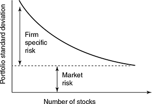
35. ‘Calibration’ is simply the process of assigning a default probability to a rating or a homogeneous segment of borrowers.
36. The ‘gamma distribution’ is a skew distribution that approximates to the normal distribution when the mean is large. This continuous probability distribution that has two parameters—a scale and a shape parameter—called α and β. It is fully described by its mean µ and standard deviation σ, such that µ = αβ and σ² = αβ². It is prevalently used in engineering, science and business to model continuous variables that are always positive and have a skewed distribution. Examples of its use include ‘queuing’ models—such as estimating the flow of material in manufacturing and distribution processes, assessing the load on web servers and applications in telecom exchanges. Its skewed profile makes it an appropriate model in climatology, say for rainfall pattern assessment, or in financial services, such as for modelling magnitude of loan defaults or insurance claims.
37. Stephen Kealhofer, John McQuown and Oldrich Vasicek founded KMV Corporation in 1989. Their credit risk models are based on a modification of Merton’s asset value model. The firm was subsequently acquired by Moodys corporation, and details of various versions of the model can be accessed at www.moodysanalytics.com.
38. Please refer to any standard corporate finance textbook for an understanding of ‘present value’, ‘free cash flows’ and ‘discount rate’.
39. For a discussion on the Equity Multiplier, a measure of ‘leverage’ and the impact of debt on a firm’s balance sheet, please refer to chapters on ‘Bank financial statements’ and the annexure containing ‘financial ratios’ in the chapter on ‘Uses of funds—the lending function’.
40. ‘Options’ are discussed in detail in the chapter on ‘risk management’.
41. Fischer Black and Myron Scholes ‘The pricing of options and corporate liabilities’, Journal of Political Economy 81, no. 3 (May–June 1973): 637–659.
42. Robert C Merton, ‘On the Pricing of Corporate Debt: The Risk Structure of Interest Rates.’, Journal of Finance. 29, no. 2 (May 1974): 449–470.
43. Fischer Black and John Cox, ‘Valuing Corporate Securities: Some Effects of Bond Indenture Provisions’, Journal of Finance 31, no. 2 (May 1976):351–36
44. There are two basic types of options, ‘call’ and ‘put’. A ‘call’ gives the option holder the right to buy the underlying asset for the strike price, whereas a ‘put’ gives the option holder the right to sell the underlying asset for the exercise price.
45. A random variable X is ‘lognormal’ if its natural logarithm Y = log(X ) follows a normal distribution. This means that Y is a normal distribution with mean µ and variance σ². It is prevalently used in modelling stock or volatile asset prices where we assume that asset returns are normally distributed.
46. The Modigliani–Miller theorem is a Nobel Prize winning proposition that states that under perfect market conditions, the value of the firm is independent of its capital structure. Refer M. Miller and F. Modigliani, ‘The cost of capital, corporation finance and the theory of investment,’ American Economic Review (June 1958).
47. The term structure of interest rates is discussed in the chapter on ‘Risk management’.
48. A ‘stochastic process’ is simply a collection of random variables—variables whose values change in an uncertain manner—taking values in a common time space. A diffusion type stochastic process is one modelled in continuous time. Many statistical inferential problems can be described in terms of diffusions, through forming stochastic differential equations.
49. Merton in his 1974 paper (page 450) refers to the stochastic differential equation dV = (αv – C)dt + σVdz, where α is the instantaneous expected rate of return on the firm per unit time, C is the total dollar payouts by the firm per unit time to either its shareholders or liabilities-holders (e.g., dividends or interest payments) if positive, and it is the net dollars received by the firm from new financing if negative; σ² is the instantaneous variance of the return on the firm per unit time and dz is a standard Gauss––Wiener process. For more on the Gauss––Wiener process, please refer to a standard book on statistics.
50. European call options can be exercised only on the maturity date of the option. If the option can be exercised at any time before maturity, it is an ‘American option’. Options basics are discussed in the chapter on ‘risk management’.
51. Also called the KMV–Merton model, the KMV–Merton model was developed by the KMV Corporation in the late 1980s. It was successfully marketed by KMV until KMV was acquired by Moodys in April 2002. The model is now sold to subscribers by Moody’s Analytics Enterprise Risk solutions.
52. Peter J Crosbie and Jeffrey R.Bohn ‘Modelling default risk’, KMV LLC, 2002.
53. Ibid, 3.
54. Moodys KMV company, 2006, ‘Structural Modelling in Practice’, presentation by Dr. Jeffrey R Bohn, Head of Research, Moodys KMV company.
55. Crosbie, Peter J, and Bohn, Jeffrey R, 2003, ‘Modelling default risk—Modelling methodology’.
56. Ibid, 13
57. Ibid, 13, Figure 8.
58. Assume that firms with DD = 4 number 6000 at a particular point in time. Also assume that 20 firms out of these defaulted after one year. Then EDF 1st year = 20/6000 = 0.0033 = 0.33 per cent or 33 bps.
59. Sources: Moody’s Analytics, June 2012, ‘Public Firm Expected Default Frequency (EDFTM ) Credit Measures: Methodology, Performance, and Model Extensions’ (Modelling Methodology), and Dwyer, d, Qu S, 2007, EDF™ 8.0 MODEL ENHANCEMENTS, Modeling methodology
60. www.moodysanalytics.com
61. The technical document of Credit Risk+™ can be accessed at http://www.csfb.com/institutional/research/assets/creditrisk.pdf, accessed on 21 April 2009.
62. In the context of two state models, a typical approach is by means of Bernoulli random variables.
63. In its simplest form, a Poisson distribution assumes that every borrower can have multiple defaults, as contrasted with the Bernoulli distribution given earlier, which assumes that there are only two outcomes—the counter party either defaults or survives. One of the essential assumptions of the Credit Risk+ model is that the individual probabilities of default are sufficiently small for the compound Bernoulli distribution of default events to be approximated by a Poisson distribution.
64. Derived from the PGF for a portfolio of independent borrowers/counter parties, explained in the Credit Risk+™ document, Appendix A (1997): 34–35.
65. Based on the information in Credit Risk+™ document, Appendix A (1997): 33.
66. We can illustrate the PGF through a numerical example. If there is a portfolio X with only one borrower, who has a probability of default of, say, 5 per cent over the next 1 year, the number of defaults over the next 1 year will have a probability distribution as follows: P (X defaults, i.e., X = 1) = 0.05 and P (X does not default, i.e., X = 0) = 0.95. The PGF would be P(z) = 0.95z⁰ 1 0.05z¹. This is the PGF defined in Credit Risk+ technical document, Appendix A, equation (3), page 34. The same numerical example can be presented in a different way. If the portfolio value is defined as the expected exposure loss, then X will have the probability distribution at the end of one year as P(X defaults, recovery = 0) = 0.05 and P(X does not default, recovery = 5, say by way of interest + principal) = 0.95. Now the PGF would be P(z) = 0.05z⁰ + 0.95z⁵.
67. The numerical example in the previous footnote will help understanding this notation.
68. Philippe Artznerand and Freddy Delbaen ‘Default Risk Insurance and In-Complete Markets’, Mathematical Finance 5 (1995): 187–195.
69. Robert A. Jarrow and Stuart M. Turnbull, ‘Pricing Derivatives on Financial Securities Subject to Credit Risk’, Journal of Finance 50, no. 1 (1995): 53–86.
70. Darrell Duffie and Kenneth J. Singleton, ‘Modelling Term Structures of Defaultable Bonds’, Review of Financial Studies 12 (1999): 687–720.
71. The interested reader can access the mathematical derivations from the papers quoted above, as well as subsequent work and books by the above researchers and others.
72. If the default process N_T had a zero trend, that is, the calculation agent (by a specified valuation method). In expected future default given current information is exactly the current value of the process, it would be a ‘fair game’ or a ‘martingale’.
73. D. Madan and H. Unal, ‘Pricing the Risks of Default’. Review of Derivatives Research 2 (1998), 121–160.
74. Robert A. Jarrow, David Lando and Stuart M Turnbull, ‘A Markov Model for the Term Structure of Credit Risk Spreads’, The Review of Financial Studies 10, no. 2 (Summer 1997): 481–523.
75. These documents are available at http://www.kamakuraco.com.
76. The basic form of this model can be found in Chava, Sudheer and Robert A Jarrow (2004), ‘Banruptcy prediction with industry effects’, downloaded from http://ssrn.com, accessed on 2 May 2009.
77. Source: Kamakura Corporation, June 2011, ‘Implied credit ratings- Kamakura public firm models’, Version 5.0, pages 9, 10
78. Robert A. Jarrow and Philip Protter, ‘Structural Versus Reduced Form Models: A New Information Based Perspective’, Journal of investment management 2, no. 2 (2004): 1–10.
79. Ibid, 8
80. According to the British Bankers’ Association (BBA) 2006 credit derivatives survey, the largest contributor to CDS growth has been CDS Index trading. The survey points out that about two-thirds of banks’ derivatives volume is from trading activities. Unlike credit insurance contracts, credit derivatives are negotiable and attract large secondary trading. The Chicago Board of Trade has introduced CDR Liquid 50 NAIG Index futures contract, which enables the CBOT to facilitate growth of the CDS market. More information on CDS trading can be accessed at www.cbot.com. In addition, Creditex has online trading platforms for credit derivatives (www.creditex.com).
81. Wai-Yan Cheng, ‘Recent Advances in Default Swap Valuation’, Journal of derivatives (Fall 2001): 18–27.
82. Credit events that trigger a default swap may include one or more of the following: failure to meet payment obligations when due, bankruptcy, repudiation, material adverse restructuring of debt, obligation acceleration or obligation default. These are as defined by ISDA.
83. One basis point is (1/100) per cent.
84. Default swap spreads, though economically comparable to bond yield spreads, do not require specification of a benchmark risk-free yield curve. Second, changes in credit quality get reflected faster in CDS spreads than in bond yield spreads. Hence, CDS spreads are able to reflect credit risk with more speed and accuracy.
85. A loan (or bond) is a deliverable obligation if it has a maturity less than 30 years, is a G6 currency, and not subordinated to the reference asset (for more details, see the ISDA Web site).
86. The final price is the market value of the reference obligation on the default date as computed by a specified calculation agent (by a specified valuation method). In practice, one or more dealers are asked for quotes on the reference obligation. Of the quotes obtained, the highest and the lowest quotes are ignored. The average of the remaining quotes is considered the value of the reference obligation.
87. D. Duffie, ‘Credit Swap Valuation’, Financial Analysts Journal (January/February 1999): 73–87.
88. Please refer to Box 9.1 in Section II of this chapter for the distinction between risk neutral and real world probabilities.
89. From here on, we follow the approach of Hull and White (2000) in their paper Hull J. and A. White, ‘Valuing Credit Default Swaps I: No Counter party Default Risk’, Journal of Derivatives 8, no. 1 (Fall 2000): 29–40.
90. Arbitrage is the simultaneous purchase and sale of an asset, in different markets or in different forms, in order to profit from a difference in the price. Arbitrage exists as a result of market inefficiencies; it provides a mechanism to ensure prices do not deviate substantially from fair value for long periods of time. The ‘no arbitrage’ argument in valuing CDS is explained in detail in Hull J. and A. White, ‘Valuing Credit Default Swaps I: No Counter party Default Risk’, Journal of Derivatives, (Fall 2000): 29–40.
91. In accordance with the practice in the interest rate swap market, the protection buyer is the ‘fixed rate’ payer, while the protection seller is the ‘floating rate’ payer. The protection buyer is also indicated by terminologies, such as (a) long CDS, (b) CDS buyer, (c) credit risk seller and, (d) fixed rate payer; while the protection seller is also called (a) short CDS, (b) CDS seller, (c) credit risk buyer and (d) floating rate payer. Another thing to remember is that with CDS, buying protection is ‘short’ the reference asset and selling protection is ‘long’ the reference asset. This is because buying protection implies ‘selling’ the reference asset. The market value of the premium leg acts like a short in that as the price of the CDS falls, the market value of the trade increases. The opposite is applicable to the protection leg.
92. J. C. Hull and Alan White, ‘Valuing Credit Default Swaps II: Modelling Default Correlations’, Journal of derivatives 8 (2001): 12–21.
93. R. A. Jarrow and S. M. Turnbull, ‘Pricing Derivatives on Financial Securities Subject to Credit Risk’, Journal of Finance 50 (1995): 53–85.
94. Dominic O’Kane and Stuart Turnbull, ‘Valuation of Credit Default Swaps’, Fixed Income quantitative research, Lehman Bros, QCR Quarterly, vol 2003-Q1/Q2 (2003): 1–19. The model is illustrated through easy to understand numerical examples.
95. Binomial tree is used in pricing options.
96. D. Duffie and K. J. Singleton, ‘Modelling Term Structure of Defaultable Bonds’, Review of Financial Studies. 12 (1999): 687–720.
97. Note that ‘conditional probabilities’ are also called ‘default intensities’, which form an important part of the reduced-form models discussed in the previous section.
98. There are two ways to price risky (defaultable) debt—one is to discount the risky (default-adjusted) cash flows by the risk-free rate, and the other, to discount risk-free cash flows by risk-adjusted (default spread) rates. Since we do not know the risky rates, it is easier to price the debt by discounting risky cash flows with the risk-free rate, which is easier to obtain or infer. On the other hand, calculating of risky cash flows is also simple—this is the expected cash flow based on probability of default. This is the reason for wide usage of the risk-free rate in the pricing methodology.
99. ‘Swaps’ in general is discussed in the chapter on ‘Risk management in banks’.
100. A good resource to understand cash flow and market value CDOs is the ‘CDO Handbook’ published by J P Morgan Securities Inc (2002).
101. This sample CDO structure can be found in ‘Markit Credit Indices: A Primer’, Markit group Ltd., May 2009, accessed at www.markit.com on 16 May 2009.
102. Based on the example given in ‘Markit Credit Indices: A Primer’, published in May 2009, accessed at www.markit.com.
103. After the financial market collapse in 2007, this method too has drawn flak, and has been named as one of the reasons for the miscalculation by investors. However, for those interested in an analysis of this approach, please refer Christopher Finger, ‘Issues in the Pricing of Synthetic CDOs’, Risk metrics Group, working paper 04–01 (2004), at www.riskmetrics.com.
104. Summarized from Padmalatha Suresh ‘Credit Derivatives—Still Relevant?’, Treasury Management, The ICFAI University Press, (March 2009): 36–42.
105. 2008, Survey of credit underwriting practices, Office of the comptroller of currency, USA.
106. The term ‘underwriting standards’, as used in the above report, ‘refers to the terms and conditions under which banks extend or renew credit, such as financial and collateral requirements, repayment programs, maturities, pricing and covenants. Conclusions about ‘easing’ or ‘tightening’ represent OCC examiners’ observations during the survey period. A conclusion that the underwriting standards for a particular loan category have eased or tightened does not necessarily indicate that all the standards for that particular category have been adjusted.’
107. ‘Survey of credit underwriting practices, 2008’, Office of the comptroller of the currency, USA (June 2008).
108. Information gathered from various sources, notably “Credit Default Swaps: Past, Present and future”, a paper by Patrick Augustin et al, published in the Annual Review of Financial Economics, August 2016, and www.bis.org.
109. The full text can be accessed at http://www.cftc.gov/idc/groups/public/@swaps/documents/file/hr4173_enrolledbill.pdf
110. The full text can be accessed at HTTP://EUR-LEX. EUROPA.EU/LEGAL-CONTENT/EN/TXT/PDF/?URI=CELEX:32014L0065&FROM=EN
111. All the Basel documents can be accessed at www.bis.org
112. Accessed at http://www.bis.org/publ/qtrpdf/r_qt1706b.htm
113. Select references: McKinsey and Company, March 2013, ‘Making data analytics work: Three key challenges; Burton, Dominic, and Court, David, 2012, ‘Making Analytics work for you’, Harvard Business Review, October 2012
114. Author: Ganesh S. About Author: Is a mentor of an Initiative named Campus Levers started by an alumni group of Indian Institute of Management, Calcutta (IIMC). The initiative is aimed at supporting academic institutes and the student community to understand the real business world with aid of systems and tools that impart business learning in a practical way.
115. Freddie Mac, the acronym for the ‘Federal Home Loan Mortgage Corporation’ (FHLMC), is a governmentsponsored enterprise (GSE) of the US federal government. Its primary objective is to expand the secondary market for mortgages in the United States. It buys mortgages on the secondary market, pools and packages them, and sells them as mortgage-backed securities (MBS). In September 2008, consequent to its role in the credit crisis, the federal government took over Freddie Mac and Fannie Mae (Federal National Mortgage Association), the other mortgage loan purchaser in the private sector. In 2008, both institutions together owned or guaranteed about half of the US’ $12 trillion mortgage market. Hence, both were at high risk from the subprime crisis.