
CHAPTER TEN
Managing Market Risk—Banks’ Investment Portfolio
CHAPTER STRUCTURE
Section II Measuring Market Risk with VaR
Section III Banks’ Investment Portfolio in India—Valuation and Prudential Norms
KEY TAKEAWAYS fROM THE CHAPTER
- Understand the primary objectives of banks’ investments.
- Know the functions of the bank treasury.
- Learn about conventional and contemporary treasury products.
- Understand risks associated with the treasury.
- Learn some tools for market risk measurement such as the VaR and the Expected Shortfall (ES), and how international regulations use them.
SECTION I
BASIC CoNCEPTS
We have seen in the chapter ‘Banks Financial Statements’ that ‘investments’ constitute a major asset on banks’ books and along with ‘loans and advances,’ take up a major share in banks’ total assets. We have also seen in an earlier chapter the rationale for bank credit and its key role in a country’s economic growth. If credit growth is a major driver of economic growth then what part do ‘investments’ play in banks’ larger role as financial intermediaries?
Typically, banks invest in securities to meet the following objectives:
Safety of Capital We have seen that substantial credit risk is attached to the loan portfolio of banks. To offset this risk, banks invest in securities with low default risk thus preserving the capital.
Liquidity Banks need adequate liquidity to pay off unanticipated demands from the depositors and other liability holders, as well as meet the loan demands. In case a bank does not have liquid funds at the time these demands are made, it has two options—it can borrow from the market or it can sell off near cash assets. Market borrowings carry an inherent risk—interest rates at the time of borrowing may be more than the cost of deposits to be repaid or the contracted yield on the loans. This is called ‘interest rate risk’ and can lead to earnings volatility. On the other hand, banks can invest surplus funds in marketable securities, which can be liquidated in the short term. However, if the market value of these investments at the time of liquidation is less than the book value, the bank will have to report a loss. If the banks decide to invest in low rate securities with fairly stable market values, there is an opportunity loss in the form of reduced interest income.
Yield From the above point, it follows that banks will have to make investments in securities that will also yield reasonable returns. However, paradoxically, higher returns will flow from investments with higher risk. Portfolio managers will, therefore, have to look at risk return trade offs while building the investment portfolio of the bank.
Diversification of Credit Risk Over time, banks develop expertise in lending to a specific sector or industry and find it difficult to diversify their loan portfolios. Hence, banks invest in securities spanning diverse geographic areas or industries to offset credit risk, as well as ensure safety of the capital invested.
Managing Interest Rate Risk Exposure Banks can easily and quickly adjust the maturity or duration (refer chapter on ‘risk management’) of their securities portfolio in times of interest rate volatility. This flexibility will not be typically available with loan portfolios.
Meeting Pledging Requirements Most bank borrowings can be collateralized with assets and marketable securities are accepted as qualifying collateral.
From the foregoing discussion, it is evident that a bank’s investment portfolio cannot satisfy all the objectives. There may be circumstances under which a bank looks for yield from security investments to bolster its dwindling spreads on loans made. There could be other times at which the bank’s liquidity needs would be overarching. How should then the investment portfolio of banks be balanced? Regulators in most countries deal with this dilemma by stipulating that banks hold their investments in three classes to satisfy most of the objectives given above.
Typically, regulators stipulate that banks divide their security holdings into three categories, based on the objectives of such investment as given below.
- Held to maturity (HTM): These are securities purchased with the objective of holding till maturity. On the balance sheet, they are carried at a mortised cost (historical cost adjusted for principal payments). The capital gains or losses at the time of maturity will be taken to the income statement. However, during the period they are held, unrealized gains or losses due to market fluctuations have no impact on the income statement.
- Held for trading (HFT): These securities are purchased with the intention to sell in the near term. They are carried at market value on the balance sheet, and therefore, unrealized gains or losses could impact the income statement.
- Available for sale (AFS): Securities not classified under the above two categories will be included here. They too are carried at market value on the balance sheet.
It is evident that the above classification based on the motive of investment determine the accounting impact on banks’ financial statements. For instance, a fixed rate bond (without options) will sell at par if the market rates and the coupon rate on the bond are the same. If market rates rise above the coupon rate, the market value of the bond falls below the par value. If market rates fall, the reverse would happen. Thus, the difference between the market value and par value would be the unrealized1 gain or loss on the security.
However, if the intention is to hold the bond until maturity, changes in interest rates and the unrealized gains or losses will not affect the value of the security in the bank’s financial statements.
Therefore, prudential treatment requires that adequate provisions are made in the income statements for unrealized gains or losses based on market values in the case of securities held by the trading categories.
The Treasury Functions
A bank’s ‘treasury’ is a source of substantial profit to the bank and can therefore create substantial value to shareholders. In addition to managing liquidity, the treasury is responsible for managing assets and liabilities, trading in currencies and securities, and developing new products. High-performing treasuries systematically identify and mitigate profit from market risk—the risk arising from changes in interest rates, exchange rates and the value of securities and commodities. Banks’ treasuries typically perform the following basic functions within their investment and trading activities.
- Investment advice and assistance to customers, including other banks, to manage their investment portfolios. Most treasury products are associated with the credit-and cash-management needs of corporate customers (for example, off balance-sheet and tax-efficient loans or project finance).
- The treasury can also play an important role in structuring products to hedge the bank’s own capital. These products—typically derivatives contracts—protect the bank’s capital exposure to a particular currency or to market factors such as, changing interest rates and commodity prices.
- The treasury buys and sells securities on behalf of the customers. The willingness of the treasuries to buy and sell securities is also called ‘making the market’. While making the market, they also make profits on the transactions by maintaining a positive spread between the ‘bid’ (buy) and ‘ask’ (sell) prices. Large banks are also market makers in options and interest rate swaps.
- Banks, as traders, also speculate on short-term interest rate movements. The bank’s treasury may borrow in US dollars and lend in the rupee inter-bank market or vice versa to take advantage of the domestic and foreign interest rates. Alternatively, the treasury could borrow in the short-term money market2 and invest in ‘commercial paper’. When the treasury expects interest rates to rise (bond prices to fall), it goes ‘short’ (sells securities) to avoid holding assets expected to depreciate in value. Conversely, when the Treasury expects interest rates to fall (bond prices to rise), it goes ‘long’ (buys securities).
- Treasury departments act as risk managers for banks. By using sophisticated internal transfer pricing, the treasury buys and sells funds among the bank’s client-facing units, thus isolating and removing maturity and interest rate mismatches from corporate and retail business units. The treasury determines prices of ‘buying’ and ‘selling’ resources by business units of the bank on the basis of market rates of interest, the cost of hedging market risk and the cost of maintaining reserve assets of the bank. For instance, the bank branches may source deposits at, say, 6 per cent and transfer it to the treasury at ‘market cost’, which could be, say, 5 per cent after adjusting for hedging and liquidity. The difference of 1 per cent is borne by the deposit mobilizing units. Similarly, treasury ‘sells’ resources to the lending branches of the bank at 7 per cent, while the branches lend these resources at 10 per cent in the market. The difference of 3 per cent represents the risk premium earned by the lending units.
As markets develop, many credit products are being replaced by treasury products. An example is working capital credit being substituted by commercial paper. Loans are being converted into tradable securities through securitization. Since treasury products are more marketable, liquidity can be infused when required.
Features of Treasury Profit The following are the features of treasury profit:
- Treasury operates in markets that are almost free of credit risk.
- Treasury operates with little capital allocation, but the upside potential is unlimited, that is, the returns on capital could be very high.
- Operating costs are lower than for branch banking, whether corporate or retail.
- The treasury is manned by a few specialists, but the value of transactions could be very high.
- Business volumes are substantial to compensate for the thin spreads in trading.
Sources of Treasury Profit
1. Foreign exchange business: Buying and selling foreign currency to customers is a source of non-interest income for banks. The difference between the ‘bid’ and ‘ask’ rates, called the spread, constitutes the banks’ profit. Banks buy foreign currency from exporter customers and sell the foreign currency in the inter-bank market. They can also sell the foreign currency to customers (importers), for which they can buy the currency in the inter-bank market or use the currency bought from exporter customers. Banks buy and sell in the inter-bank markets to square the foreign currency balances at the end of each day. Thus, banks do not maintain a stock of foreign currency at the end of each day. In case, a bank maintains an open position (overbought or oversold) at the end of any day, it exposes itself to exchange risk (adverse changes in the value of currency overnight).
New treasury products in the foreign exchange markets have considerably widened the range of services that the banks offer. These markets are the most liquid in respect of currencies that can be freely bought and sold, such as US dollars, Euros and Sterling pounds. These markets are also transparent markets, since information on currency movements are freely available. They are virtual markets with little or no physical boundaries and effective information dissemination. Hence, foreign exchange markets are likened to near-perfect markets with an efficient price discovery mechanism.
Some of the prevalent treasury products3 in these markets are listed below:
- Spot trades, referring to current transactions, where mostly currency is bought and sold.
- Forward and futures trades, involving purchase or sale of currency at a future date.
- Swaps, which are a combination of spot and forward transactions. Though the swap is generally used for funding requirements, there is also a profit opportunity from interest rate arbitrage.
- Investment of foreign exchange surplus, which could arise out of profits from treasury or overseas branch operations, borrowings or deposits in foreign currency in global money markets or short-term securities.
- Loans and advances in foreign currency.
- Foreign bills rediscounting in the inter-bank market.
2. Money market products: These are securities with short maturities and durations, typically 1 year or less. They are held to meet liquidity and pledging requirements and also for a reasonable return.
Some of the prominent ‘money market’ products are as follows:
- Repurchase agreements or repo: These represent a loan transaction between two parties, typically securities dealers and banks. The lender (investor) buys securities from the borrower, simultaneously agreeing to sell the securities back on a predetermined date at a predetermined price plus interest. The borrower receives funds, while the lender earns interest on the investment. The underlying securities form the collateral for the loan. If the borrower defaults, the lender gets title to the securities. Banks operate both as lenders and borrowers in the repo market and the collaterals are typically government securities (though any security can serve as collateral) (Also refer chapter ‘Monetary policy implications for bank management’).
- Treasury bills or T-bills: These securities are marketable obligations of the government, carrying maturities of one year or less. They are attractive to banks because they are highly liquid, free of default risk, offer reasonable rates of interest and are tradable in the secondary market. The prices of T-bills are determined through an auction process in which banks participate. Banks can buy the bills directly for their own investment portfolios or for their trading activity. T-bills are purchased at a discount and the discount rate is quoted in terms of a 360 day year as being equal to (face value—purchase price) × (360/number of days to maturity)/face value.
- Commercial paper (CP): These are unsecured promissory notes issued by corporations for the purpose of financing short-term working capital requirements. There are two types of CPs—’direct paper’ and ‘dealer paper’. Direct paper is issued primarily by finance companies and bank holding companies, while dealer paper (also called ‘industrial paper’) is issued primarily by non-financial firms through securities dealers. The CP issuers have to be highly creditworthy firms, since these instruments are not backed by any collateral. Most CP issues are rated by external rating agencies to signify the default risk. Banks invest in CPs since they typically yield more than T-Bills.
- Certificates of deposit (CD): These are negotiable debt instruments similar to CPs, the difference being that they are issued by banks against deposit of funds. They are attractive because they yield more than T-bills do and if issued by a prime bank, can be sold in the secondary market before maturity. Even though CDs are issued by creditworthy banks, investors usually demand a risk premium over the deposit rates offered by safe banks. Recently, banks have also started offering stock market indexed CDs, where the interest rate is linked to the stock market index of the country.
- Bankers’ acceptances (BA): These are products predominantly used in international trade financing. A banker’s acceptance simply represents a draft drawn on a bank by an exporter or importer of goods and services. The draft represents an order to pay a specified amount of money at a predetermined future date. When the bank ‘accepts’4 this draft, it represents a guarantee from the accepting bank to remit the face value of the draft at maturity. Bankers’ acceptances are negotiable instruments and are mostly associated with letters of credit.5 For the investor, BA represents a short-term interest bearing draft accepted by a prime bank. Due to the low default risk, the rate is only slightly above that of a T-Bill of comparable maturity.
3. Securities market products: Banks’ investment portfolios are typically dominated by securities that can be bought and sold in the government securities and capital markets. Each of these securities exhibit varying risk and return features. In most countries, regulations restrict banks’ investments to ‘investment-grade’6 securities only.
- Government securities: These are long-term securities issued by the governments of various countries for financing social programs. They are perceived as risk free, are highly liquid and carry attractive coupon rates. Like T-bills, government securities are sold through auctions and are actively traded in secondary markets. Box 10.1 outlines the salient features of some capital market instruments in the US.
BOX 10.1 US GOVERNMENT SECURITIES
There are four major types of marketable securities issued by the Department of Treasury in the US namely, bills, notes, bonds and treasury inflation protected securities (TIPS). These are direct obligations of the government and are considered free from default risk.
Treasury bills are issued for very short maturities, not exceeding a year. They are issued at a discount. The interest earned by the bank is the difference between the face value paid at maturity and the discount price.
The US treasury issues treasury notes, which are interest bearing notes with original maturities of 1–10 years. The prices and yields on these notes are set through auctions and investors include pension funds, insurance companies, financial institutions, corporate bodies and some foreign institutions. The secondary market for these securities is extremely deep, due to the large volumes being traded, low default risk and wide range of investors. In addition, thirty year bills or STRIPS (Separate trading of registered interest and principal of securities) are permitted by the US Treasury. STRIPS are created out of standard T-bills, treasury notes and bonds and are issued as bearer instruments. These instruments are ‘stripped’ into their interest and principal components and traded as ‘zero coupon’7 securities. Each zero coupon security is priced by discounting the promised cash flow at the appropriate interest rate. Banks find these instruments attractive since they are assured of fixed interest payment and yield for the selected maturity. Further, as there are no interim cash flows, there is no reinvestment risk. For example, a 10 year USD 10 million par value treasury bond that pays 10 per cent coupon interest (5 per cent semi-annually) pays USD 500,000 semi-annually. Thus, this security can be ‘stripped’ into 20 disparate interest payments of USD 500,000 each and a single USD 10 million payment at the end of 10 years or 21 separate zero coupon securities. If the market rate on the 3 year zero coupon security is 9 per cent, the associated price of the zero related to the sixth semi-annual payment would be 500,000/(1.045)6 or USD 383,949.
The US Treasury created TIPS in 1997. TIPS pay a fixed rate of interest semi-annually on the inflation adjusted principal amount. The amount paid out as interest will be calculated as the annual interest rate multiplied by the adjusted principal. Since the principal is adjusted for inflation, its value may fluctuate. But, at maturity, the greater of the face value or the inflation adjusted principal is paid. These securities are also eligible for the treasury’s STRIPS.
In addition, banks in the US also invest in government agency securities, which exhibit characteristics similar to those of the US treasury securities. Agency securities are interest bearing and are issued at a discount to the face value. However, the agency securities are less liquid, since the issues are much smaller than treasury issues. Further, unlike treasury securities, agency securities may not be backed by federal government and may not be eligible for tax exemptions. Therefore, in order to compensate for these risks, the returns on agency securities are higher than treasury securities.
Other investments by banks in the US capital market include mortgage backed securities (MBS) that exhibit characteristics similar to corporate bonds. An MBS is a security that evidences an undivided interest in the ownership of mortgage loans. The most common form of MBS is the ‘pass-through security’,8 in which homogenous mortgages are pooled and investors buy an interest in the pool in the form of securities. Other popular forms of MBS are: (a) Government National Mortgage Association, known as Ginnie Mae or GNMA pass-through securities, (b) Federal Home Loan Mortgage Corporation, popularly termed as Freddie Mac or FHLMC participation certificates, guaranteed mortgage certificates and collateralized mortgage obligations, (c) Federal National Mortgage Association, popularly termed as Fannie Mae or FNMA securities, and (d) other privately issued pass-throughs.9
- Corporate debt paper, debentures and bonds: These are debt instruments issued by the corporate bodies, mostly secured by specific assets. They may be issued with differing structures in order to enhance marketability and reduce cost of issue. Some of the common variations include structured obligations with put, call or convertibility10 options, zero coupon bonds, floating rate bonds, deep discount bonds or instruments with step up coupons.
- Equities: While investing in equities, banks take direct exposure to the stock market. The risks involved in equity trading is matched by good returns but bank treasuries are circumspect while investing in equities.
Risks and Returns of Investment Securities
The primary objective of banks’ investment portfolio and treasury operations is to maximise earnings while mitigating risks that are involved.
There are three predominant methods by which bank investments contribute to earnings, which are as follows:
- Interest income
- Income from reinvestment
- Capital gains or losses
However, the earnings are susceptible to the following risks:
- Interest rate risk is the potential volatility in returns caused by the changes in the interest rates. How do variations in earnings take place? If the bank holds fixed income securities, the market value of these securities would change in the direction opposite to the change in interest rates of comparable securities. If market interest rates (on comparable debt securities) increase after purchase, the market value of fixed-rate and option-free debt decreases.11 Second, if the interest rates are decreasing, the investor will have to reinvest the coupon payments at lower rates. This is called reinvestment risk. In most cases, it is seen that interest rate risk is offset by reinvestment returns and vice versa. For example, if interest rates rise and the treasury decides to sell the bonds at less than cost, it can recoup part of the loss by reinvesting the proceeds to earn future coupon payments at the higher rates. When rates decrease, the treasury can sell the securities at a gain. However, part of the gain is offset by the lower rates earned by the reinvested amount. Hence, interest rate risk (also called price risk) will have to be viewed along with reinvestment risk.
- Credit risk arises in case when the bank’s investment in debt securities does not yield the promised interest and principal payments. It is for this reason that many central banks require that banks invest only in ‘investment grade’12 securities, though these securities typically yield less than ‘non-investment grade’ securities. In many countries, regulators permit banks to invest in unrated securities as well, but the banks should maintain credit files on these issuers and be able to justify the economic rationale for the investment. Detailed analysis of the issuer’s creditworthiness, as for credit expansion, is required for sound investment by the bank.
- Even though one of the important objectives of maintaining investment portfolios is liquidity, investment in securities could also be illiquid at times. Liquidity risk could arise from the lack of a market for securities held by the bank. Some securities, such as those in very small lots or unrated securities cannot be easily sold before maturity. The bank may have to sell off such securities by offering considerable discounts on the price. Second, securities used for pledging requirements are illiquid in the short term, since banks will have to substitute other collateral before reclaiming the security from the pledge for sale. Third, banks are expected to hold the ‘HTM’ securities till maturity and will have to show strong justification for the need to sell such securities before maturity.
- Of other general risks that could cause volatility in returns from the investment portfolio, the most important and visible is the inflation risk. Unanticipated rise in inflation would erode the purchasing power of the return from the fixed rate securities. Investors have deferred consumption to purchase these securities, but in inflationary conditions the returns, when they are actually received, buy less. Banks’ profitability will take a hit when the banks’ inflation expectations are lower than the inflation expectations of its depositors, but the actual inflation is high. When this happens, banks would be willing to accept lower returns on its investments, as compared with what they have to pay to the depositors. The higher is the actual inflation, the worse is the banks’ spread.
SECTION II
MEASURING MARKET RISK WITH VaR AND EXPECTEd SHARTfAll (ES)
The increasing volatility of financial markets has necessitated design and development of more sophisticated risk management tools. Value at risk (VaR) has become one of the standard measures to quantify market risk.
The concept and use of VaR as a risk management tool gained prominence only about two decades ago. Major financial firms in the late 1980s were using the VaR to measure the risk of their trading portfolios. Since then, VaR has had a meteoric rise as a market risk management tool. Most derivative dealers around the world use the concept to measure and manage market risk. In 1994, J P Morgan released ‘Risk Metrics’TM as a market standard and this provided further fillip to VaR usage.
VaR is defined as the maximum potential loss in the value of a portfolio due to adverse market movements for a given probability. The conceptual simplicity of this measure has made it immensely popular. VaR reduces the (market) risk associated with any portfolio to just one number, the loss associated to a given probability. VaR is a single, summary, statistical measure of possible portfolio losses. Specifically, it is a measure of losses due to ‘normal’ market movements. Losses greater than the value at risk are suffered only with a specified small probability.
VaR measures are used both for risk management and for regulatory purposes. For instance, the Basel Committee on Banking Supervision13 at the Bank for International Settlements used to advocate VaR estimates as a basis for meeting capital requirements in banks. Box 10.2 describes the basic features of the VaR calculation.
BOX 10.2 THE RISK MEASUREMENT TOOL CALLED VaR
How the VaR evolved
It is said that J P Morgan Chairman Dennis Weatherstone used to call for a simple report at the end of each day, showing how the firm’s position would be impacted by the market risk. Analysts of J.P. Morgan evolved the VaR concept and this number was included in the ‘4.15 report’, as the report to the Chairman was called. In 1993, the Washington ‘Group of thirty’, headed by Weatherstone, recommended in its study on ‘Derivatives: Practice and Principles’ that VaR was an appropriate measure for measuring a firm’s market risk. Since then, VaR has been a very popular measure adopted by almost all financial and other institutions for reporting on market risk.
Rationale of VaR methodologies
The statistical features of financial markets have been well documented14: (a) distribution of financial market returns are leptokurtotic (in other words, they have heavier tails and higher peak than the normal distribution), (b) equity returns are negative skewed, and (c) volatilities (as measured by squared returns or standard deviations) of market factors show a cluster tendency. One or more of these empirical features form the basis of the popular VaR models.
What is VaR?
VaR summarizes the predicted maximum loss (or worst loss) over a target horizon within a given confidence interval.
How is VaR computed?
Assume a bank holds ₹100 crore in medium-term investments. How much could the bank lose in a month? As much as ₹100,000 or ₹10 lakh or ₹1 crore? An appropriate answer to this question would enable the banks to decide whether the return they receive is an appropriate compensation for risk.
In order to answer this question, we first have to analyse the characteristics of medium-term securities. Let us do this in the following steps:
Step 1: Obtain, say, monthly returns on medium-term bonds over the last 40 years. It is possible that these returns could range from a low of26 per cent to a high of +15.0 per cent.
Step 2: Construct regularly spaced ‘buckets’ going from the lowest to the highest number and count how many observations fall into each bucket (frequency distribution). Thus, we can construct a ‘probability distribution’ for the monthly returns, which counts how many occurrences have been observed in the past for a particular range.
Step 3:For each return, compute a probability of observing a lower return. This is done as follows. Pick a confidence level, say 95 per cent. For this confidence level, find on the graph a point such that there is a 5 per cent probability of finding a lower return. This number is, say,22 per cent, which implies that all occurrences of returns less than22 per cent add up to 5 per cent of the total number of months or 24 out of 480 months. (Note that this could also be obtained from the sample standard deviation, assuming the returns are close to normally distributed).
Step 4: Now, we can compute the VaR of a ₹100 crore portfolio. There is only a 5 per cent chance that the portfolio will fall by more than ₹100 crore times22 per cent or ₹2 crore. The VaR is therefore, ₹2 crore.
Step 5: In other words, the market risk of this portfolio can be communicated effectively to a non-technical audience with a statement such as: Under normal market conditions, the most the portfolio can lose over a month is ₹2 crore.
Choosing VaR parameters
In the above example, VaR was reported at the 95 per cent level over a 1 month horizon. How do we choose these two quantitative parameters?
- Horizon: If the bank’s trading portfolio is invested in highly liquid securities, even a 1 day horizon may be acceptable. For an investment manager with a monthly rebalancing and reporting focus, a 30 day period may be more appropriate. Ideally, the holding period should correspond to the longest period needed for orderly portfolio liquidation.
- Confidence level: The choice of the confidence level depends on how the bank wants to use VaR. The bank may intend to use the resulting VaRs directly for the choice of a capital cushion. In this case, the choice of the confidence level becomes crucial, as it should reflect the degree of risk aversion of the bank and the cost of a loss of exceeding VaR. Higher risk aversion or greater costs implies that a greater amount of capital should cover possible losses thus leading to a higher confidence level. On the other hand, if VaR numbers are just used to provide a yardstick to compare risks across different markets then the choice of the confidence level is not too important.
Changing VaR parameters
If we assume that portfolio returns follow the normal distribution then we can easily convert one horizon or confidence level to another.
As returns across different periods are close to uncorrelated, the variance of returns for ‘n’ days should be n times the variance of a 1 day return. Hence, in terms of volatility (or standard deviation), it can be adjusted as: VaR(n days) = VaR ( 1 day) × n
In order to convert from one confidence level to another, use standard normal tables. From these tables, we know that the 95 per cent one-tailed VaR corresponds to 1,645 times the standard deviation, the 99 per cent VaR corresponds to 2.326 times standard deviation and so on. Therefore, in order to convert from 99 per cent VaR to 95 per cent VaR,
Use of VaR
This single number summarizes the portfolio’s exposure to market risk as well as the probability of an adverse move. It measures the risk using the same monetary units as the bottom line. Investors can, therefore, decide whether they feel comfortable with this level of risk.
If the answer is no, the same process that led to the computation of VaR can be used to decide where to trim risk. For instance, the riskiest securities can be sold or derivatives such as futures and options can be added to hedge the undesirable risk. VaR also allows users to measure incremental risk, that is, the contribution of each security to total portfolio risk.
Generalizing, using a probability of ‘x’ per cent and a holding period of n days an entity’s VaR is the loss that is expected to be exceeded with a probability of only x per cent during the next n day holding period. In other words, it is the loss that is expected to be exceeded during x per cent of the n-day holding period. Typical values for the probability x are 1, 2.5 and 5 per cent while common holding periods are 1, 2, and 10 (business) days and 1 month. Values of x are determined primarily by how the user of the risk management system wants to view the VaR number is an ‘abnormal’ loss that occurs with a probability of 1 per cent or 5 per cent. For example, J P Morgan’s Risk Metrics system uses 5 per cent, while there are others who use 0.3 per cent. The parameter n is determined by the entity’s horizon. Those which actively trade their portfolios such as, financial firms typically use 1 day, while institutional investors and non-financial firms may use longer holding periods.
A VaR number applies to the current portfolio, so an implicit assumption underlying the computation is that the current portfolio will remain unchanged throughout the holding period. This may not be reasonable, particularly for long holding periods.
References: Jorion, Philippe, 2005, accessed at http://www.gsm.uci.edu/~jorion/oc/case.html and ‘Value at Risk’, Harvard Business School, (9-297-069), rev 15 July 1997.
TEASE THE CONCEPT
- A bank has a portfolio with daily VaR of ₹1 crore with 95 per cent confidence. This means that there is …… per cent chance the portfolio will lose more than ……… in the next …….. hours/days/ months.
- Can we use the VaR for simple risk comparisons? Can we, for example, compare the risk of portfolios X and Y, where both portfolios have the same value, but portfolio X’s VaR is ₹4 crore and Y’s VaR is ₹2 crore? Assume both VaR have been computed for a holding period of one month and at 99 per cent confidence interval. If they can be compared, which portfolio is more risky?
Approaches to VaR Computation
There are various approaches to VaR computation. Therefore, it is likely that firms calculating VaR for the same portfolio using different approaches may arrive at different VaR figures. Of course, each approach has its advantages, disadvantages and limitations and hence, this aspect should be borne in mind while choosing the appropriate approach and interpreting the results.
However, the approaches follow a common structure, summarized in three steps: (a) mark to market the portfolio, (b) estimate the distribution of portfolio returns and (c) calculate the portfolio VaR. Depending on the method used to arrive at (b), the models can be grouped in three categories.15
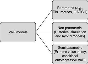
The more prevalent ones—historical simulation, the variance-covariance approach and Monte Carlo simulation—are briefly discussed below. The summary provided below is the approach for a typical, simple portfolio. The basic approach can be expanded to include more types of assets with diverse types of market risk.
The common features in all the approaches are: (a) they use historical (over long or short periods) data on the assets contained in the portfolio, (b) they value the portfolio in the next period and compare the future value with the current value and (c) they generate the distribution of the risk portfolios for the required period in future,
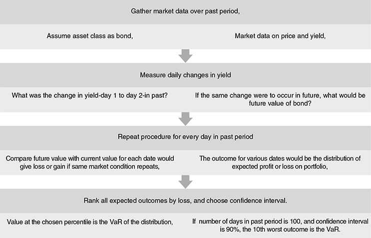
1. The Historical Simulation Approach
2. The Variance-Covariance Approach (also called the ‘analytic’ or ‘parametric’ approach) and J.P. Morgan’s Risk Metrics™
The name ‘variance-covariance’ simply signifies the covariance16 matrix of the distribution of changes in the values of the underlying market factors in the portfolio. It is based on the key assumption (there are also other assumptions) that the underlying market factors follow a multivariate normal distribution. With the normal distribution assumption, it is possible to determine the distribution of mark-to-market portfolio profits and losses, which is also normal (being a linear combination of normal variables). Return volatilities (measured by standard deviations) and correlations of risk factors are calculated using historical data. Once the distribution of expected portfolio profits and losses has been arrived at, standard mathematical properties of the normal distribution are used to determine the loss that will be equaled or exceeded x per cent of the time, i.e., the VaR.
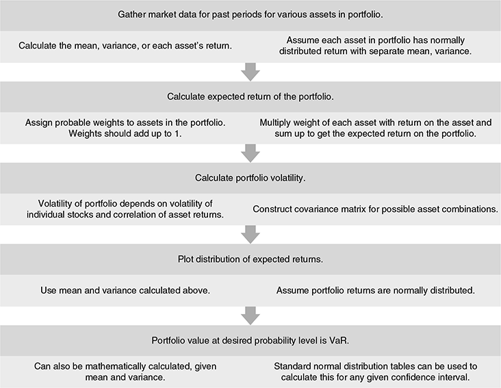
Note: As an example, the expected volatility (standard deviation) of a two-asset portfolio can be calculated using σp2 = w12σ12 + w22σ22 + 2w1w2Cov (r1, r2), where w1 and w2 are the respective asset weights in the portfolio and r and σ indicate the return and the standard deviation of the two assets, respectively. This formula can be extended to any number of assets in the portfolio.
The above approach forms the basis for the widely used Risk MetricsTM package17 popularized by J P Morgan. Box 10.3
BOX 10.3 AN OVERVIEW OF RISK METRICS ™18
In 1994, J.P. Morgan developed a VaR model primarily to support the internal reporting system called the ‘4:15 report’ that measured end of day portfolio risk. The Risk Metrics methodology was then standardized and published and developed into a software product in 1996. Two years later, Risk Metrics was spun out of J.P. Morgan as a separate company.
Risk Metrics group acquired institutional shareholder services (ISS) and Centre for Financial Research & Analysis (CFRA) in 2007. ISS was founded in 1985 to promote good corporate governance in the private sector and raise the level of responsible proxy voting among institutional investors and pension fund fiduciaries and in 1986, ISS launched its Proxy Advisory Service to assist institutional investors in fulfilling their fiduciary obligations with comprehensive proxy analysis. ISS gave Risk Metrics access to substantial data on pay, governance and other corporate practices at 41,000 companies, as well as 1,200 new clients who collectively manage $20 trillion in assets. CFRA was born in 1994 to provide institutional investors with early warning signs of business deterioration within portfolio companies. CFRA built a rigorous and proprietary forensic accounting research process for assessing the quality and sustainability of companies’ reported financial results and expanded into specialty legal, regulatory and due diligence research.
Risk Metrics is widely recognized in VaR measurement. However, the industry has yet to settle on a single industry standard for VaR calculation.
In the variance-covariance methodology outlined above, we make a critical assumption that volatility is constant. However, in practice, volatility is not constant and varies from day to day. This problem has been recognized by researchers and a widely used solution was proposed in 1986 by Tim Bollerslev that generalized the pioneering and Nobel prize winning paper of Robert Engle in 1982.19 The time varying volatility approach is commonly called the GARCH method,20 and uses heavier weights for recent returns (and their variances), than for those more distant in time (whereas the constant volatility method outlined above assumes equal weights for all squared returns—variances—in the past). However, this process of weighting calls for a complex, computer intensive procedure.
Risk Metrics is a risk management system that includes techniques to approximate GARCH volatilities. Risk Metrics uses a similar method–Exponentially Weighted Moving Average (EWMA) estimates of daily volatility that represent the weighted average of past squared returns, with the more recent returns receiving heavier weights. However, the set of weights used by Risk Metrics are easier to compute than in the GARCH methodology, and the same set of weights can be used for any asset in the portfolio–say, bonds, stocks or currencies. Similarly, for calculating covariances in the portfolio, the Risk Metrics GARCH approximation can be used to estimate time varying covariances.
Since Risk Metrics is able to yield both volatility and covariance estimates, it can also handle Monte Carlo simulation of derivative portfolios. The general view is that Risk Metrics (as well as the GARCH methodology) tend to underestimate VaR, since the normality assumption made by the model is not consistent with financial market return characteristics.
Risk Metrics has periodically been updating its computation versions—known by the year they were updated in. For example, RM 1994 indicates the methodology proposed in the year 1994. RM 2006 is the latest updated version of the methodology.
RM 1994 methodology relies on the measure of volatilities and correlations given by the historical data, using the EWMA. The appeal of this methodology is its simplicity, conceptually and computationally. However, with more understanding of and experience with volatilities, RM 2006 has introduced a process leading to simple volatility forecasts, while retaining the appeal and advantages of RM 1994. The updated version can also deal with long term horizons.
In 2010, Risk Metrics group became part of MSCI, a leading provider of investment support tools, that include indices, portfolio risk and performance analytics and governance tools. The technical document of RM 2006 is now available on www.msci.com
The appeal of the approach lies in the speed with which computations can be done and the ability to examine alternative assumptions about correlations and standard deviations.
However, the approach is limited by the normal distribution assumption, since movements in market returns do not always follow a normal distribution. The tendency of the market returns to exhibit ‘fat tails’ (extreme values or extraordinary events) can result in misleading conclusions due to the normal distribution assumption. Further, the approach has limited ability to capture the risks of portfolios containing derivatives such as options.
3. The Monte Carlo Simulation Approach
This simulation is much more rigorous than the historical simulation approach described above. It uses mathematical models to forecast future market shocks.

A comparative picture of the three most popular approaches is shown below:
| Approach | Advantages | Disadvantages |
|---|---|---|
| Variance covariance (also called parametric or analytic approach) | The least complex, hence easy to understand. | Limited ability to capture the risks of portfolios which include options, hence may misstate nonlinear risks. |
| Easy to implement for portfolios covered by available ‘offthe- shelf’ software. Ease of implementation depends upon the complexity of the instruments and availability of data. | Unable to examine alternative assumptions about the distribution of the market factors, i.e., distributions other than the normal. | |
| The least intensive computation and hence, can be done fast. | ||
| Historical simulation | Can capture risks of portfolios which include options. | May produce misleading value of risk estimates when the recent past is atypical. |
| Easy to implement for portfolios for which data on past values of market factors is available. | Difficult to perform scenario analysis under alternative assumptions. | |
| Performs well when back tested. | Can be computationally intensive. | |
| Monte Carlo simulation | Easy to implement for portfolios covered by available ‘off-the-shelf’ software. Ease of implementation depends upon the complexity of the instruments and availability of data.
Can capture the risks of portfolios which include options. Can handle statistical assumptions about risk factors Various scenarios can be tested with the model. |
The model can produce misleading values of risk estimates when recent past is atypical. However, alternative estimates of parameters may be used. |
Although VaR is being used for multiple purposes—risk reporting, risk limits, regulatory capital, internal capital allocation and performance measurement—experts opine that VaR is not the answer for all risk management challenges. The perceived shortcomings of VaR are as follows:
- It does not measure ‘event’ (say, market crash) risks. Hence, portfolio stress tests are recommended to supplement VaR.
- It does not readily capture liquidity difference among instruments.
- It does not capture model risks.
However, it is a very popular and promising tool with wide use by practitioners, regulators and academicians. Annexure I to this chapter provides a case study of the sensational collapse of LTCM and its link with VaR.
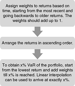
A hybrid model, which is believed to address some of the shortcomings of the popular models is also used by some practitioners. This model, developed by Boudoukh et al21 combines Risk Metrics and historical simulation methodologies. According to proponents of the approach, the results are more precise than those obtained with the other methods. The approach is implemented in three steps, which are as follows:
Some simple numerical examples of VaR applications are given in Illustration 10.1–10.3. However, before we understand the applications, we have to understand the basics of the normal distribution.
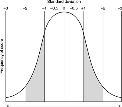
We can see from the diagram above that the normal distribution is a symmetric, bell shaped distribution, defined by its mean (µ) and standard deviation (σ). For simplicity, we assume that the mean is zero and the standard deviation is one—this is called the standard normal distribution. We also note that the distribution is symmetric around the mean—that is, the two halves of the curves are mirror images and the total area under the curve is 1 (or 100 per cent). Typically, the distribution exhibits the following characteristics:
- 68.3 per cent of the values fall within plus or minus 1 standard deviation from the mean of the distribution.
- 90 per cent of the values fall within plus or minus 1.65 standard deviation from the mean.
- 95.5 per cent of the values fall within plus or minus 2 standard deviation from the mean.
- 99.7 per cent of the values fall within plus or minus 3 standard deviation from the mean.
ILLUSTRATION 10.1 VaR FOR EQUITY SHARES OF A FIRM
A bank has recently added to its portfolio equity shares of firm ABC Ltd. The shares were bought at ₹500 per share. If the volatility of the share price is 20 per cent per annum and there are 250 trading days in a year, what is the 1 day VaR at 95 per cent confidence?
| Stock price | ₹500 |
| Volatility | 20% |
Calculate daily volatility as 20/√250 = 1.26% = σ
At 95% confidence, VaR would be
500 (1 × 2*1.26) or 500 (122*1.26)
That is, ₹512.65 or ₹487.35, which translates into a potential gain or loss of ₹12.65 per day.
ILLUSTRATION 10.2 VaR FOR FOREIGN CURRENCY (SPOT)
A bank in India has bought USD 100 million in the spot market. It would like to assess the risk of holding this position for 1 day given the volatility of the currency to be at 10 per cent per year, at the exchange rate of USD1 = ₹50 (that is, ₹1 = 1/50 USD =.02 USD). Assume 250 trading days in a year and the required confidence level at 99 per cent.
The bank’s position in ₹ is 50 × 100 million = ₹500 crore. The daily volatility is 10/√250 = 10/15.81 =.632%.
Hence, the value of the Re. to USD is likely to fluctuate between 0.02(1 + 3 ×.00632) and 0.02(1-3 ×.00632), that is between 0.0203 and 0.0196.
The bank’s position may therefore result in a loss at 99 per cent confidence level as follows:
ILLUSTRATION 10.3 VaR OF FIXED INCOME SECURITIES
The volatility of fixed income securities (such as bonds) is measured in terms of volatility in yield.
A bank has invested in fixed income bond with a price of ₹100 and coupon of 9 per cent. The market yield of a similar government security is also 9 per cent. with an annual volatility of 2 per cent. The holding period of the bank’s security is 4 months. Assume the confidence interval to be 95 per cent.
Standard deviation for 4 months = 2/√3 (since 4 months is 1/3rd of a year] = 1.15%
Hence, yields for 4 months at 95% confidence level would be
For simplicity, it can be assumed that 95 per cent of the values fall within +/-2σ and that 99 per cent of the values fall within +/-3σ. As we have seen earlier, 95 per cent, 99 per cent, etc. represent confidence intervals in the VaR calculation.
Calculations of VaR for instruments such as forwards and options are somewhat more complex.
Supplementing VaR—Stress Testing and Scenario Analysis When the VaR is exceeded, how large can the losses be?
Stress testing attempts to answer this question by performing a set of scenario analyses to assess the effects of extreme market conditions. These extreme scenarios may be hypothesized using unexpected events and their impact on the prices of instruments in the portfolio is determined If the effects are unacceptable, the portfolio or risk management strategy needs to be revised or contingency plans prepared. However, the process is more intuitive and depends substantially on the judgment and experience of the risk manager.
Scenario analyses are also used to assess the impact of assumptions underlying VaR calculations being violated.
Alternative Measures to VaR: VaR may not be appropriate for all situations or types of firms. The alternatives are sensitivity analysis, cash flow at risk and expected shortfall methodologies. Sensitivity analysis is considered less sophisticated than, and cash flow at risk and Expected Shortfall (ES) more sophisticated than VaR.
Sensitivity Analysis: Sensitivity analysis are a reasonable alternative for simple portfolios. The approach in this ubiquitous methodology is to imagine hypothetical changes in the value of each market factor, compute the value of the portfolio given the new value of the market factor and determine the change in portfolio value resulting from the change in the market factor. The methodology works well when the magnitudes of likely changes in market factors can be realistically predicted.
Cash Flow at Risk: Risks inherent in operating cash flows are captured reasonably well by this measure and hence is preferred by non-financial firms
Cash flow at risk measures are typically estimated using Monte Carlo simulation but with differences from the use of Monte Carlo simulation to estimate VaR. First, the time horizon is much longer in cash flow at risk simulations. Second, the focus is on cash flows, not changes in mark-to-market values. Third, operating cash flows are the focus of the calculation. Hence, the factors included in the simulation are not the basic financial market factors included in VaR, but those factors affecting operating cash flows such as changes in customer demand or the outcomes of advertising programs. Finally, the primary emphasis is on planning (as opposed to control, oversight and reporting).
There is high degree of subjectivity involved in this approach since successful design and implementation of a cash flow at risk measurement system presupposes substantial knowledge and judgment in respect of the firm’s operating cash flows and the important factors impacting these cash flows and then fitting these into an appropriate and workable model.
Expected Shortfall (ES): This method has been proposed as an alternative to VaR and is designed to measure the expected value of portfolio returns, given that the VaR (or some threshold) has been exceeded. The distinction between VaR and ES has been found to be not very important if the loss distribution is normal. However, for nonnormal distributions, VaR and ES can yield quite different results.
As an example, assume that two firms A and B have invested in portfolios with 1 day VaR of ₹1 crore at 95 per cent confidence level. The ES is concerned with what happens on 5 per cent of the days when the loss exceeds ₹1 crore. For firm A, the loss during this period ranges between ₹1 crore and ₹3 crore with an average of ₹2 crore. For firm B, the loss may range from ₹1 crore to ₹5 crore with an average of ₹3 crore. This implies that firm B’s portfolio is riskier even though the two firms have the same VaR. The ES has brought out the comparative risks of both firms in absolute terms.22
Expected Shortfall has found favour with the Basel Committee as a better measure of market risk in its recently published standards on minimum capital requirements for market risk. Annexure II provides a synopsis of this and other international standards and regulations.
ES and VaR – a comparison
ES will be replacing VaR when the current market risk regulations come into force in 2019 (see Annexure II). The following are cited as the limitations of VaR as a risk measure:
- The measure gave no information about the amount of loss exceeding the VaR, hence extreme losses could not be estimated
- VaR considered short term data that could “forget” past disasters (for example, the financial crisis)
- The VaR does not satisfy the required mathematical property called subadditivity, which means that in some cases it does not reflect the risk reduction from diversification effects
- The Stressed VaR (S-VaR) which replaced the VaR briefly post the financial crisis, was still a non sub additive measure that did not take into account extreme losses
ES scores over VaR since it is considered to have better theoretical properties than VAR. If two portfolios are combined, the total ES usually decreases, reflecting the benefits of diversification. In contrast, the total VaR could increase after combining two portfolios. Experts consider ES to be a “coherent” measure due to this property
A drawback of the ES measure is that it is difficult to back test. For example, when a one day 99% VaR model based on recent historical data is back tested, the number of exceptions can be observed, and can be tested for significant variations from what was expected. However, back testing a one day ES model poses challenges since the average size of the losses have to be computed when exceptions are observed.
According to some researchers, estimates of ES measure may not be as accurate as estimates of VaR.23
But the most severe limitation would be the requirement of data for calculating the ES. Data would be required over a long period to get a reasonable estimate of ES.
Did VaR and Other Such Measures Fail During the 2007–2008 Global Financial Turmoil? It has been pointed out that banks, which used VaR as a primary tool of market risk management, failed, while derivative exchanges, which deal with more complex products, did not. Derivative exchanges have moved away from VaR and used the standard portfolio analysis of risk (SPAN) system. SPAN was developed by the Chicago Mercantile Exchange in 1988 and is used to calculate the portfolio loss under several price and volatility scenarios.
SECTION III
BANKS’ INVESTMENT PoRTfolIo IN INdIA—VAlUATIoN ANd PRUdENTIAl NoRMS’24
Similar to the loan policy that sets the direction for the credit portfolio of banks, an investment policy needs to be in place with the Board’s approval. According to the RBI, the investment policy should be ‘implemented to ensure that operations in securities are conducted in accordance with sound and acceptable business practices’.25 Further, the central bank advocates that banks wanting to invest in the equity/bond markets should not only have a transparent policy for such investment but all direct investment decisions should be taken by the investment committee of the Board, which will be held accountable for the investment decisions. The central bank would like to see the banks build up adequate internal equity research capabilities.
In short, the RBI has prescribed that the investment policy of bank should clearly lay down the broad investment objectives to be followed while undertaking transactions in securities on their own investment account and on behalf of clients, clearly define the authority to put through deals, procedure to be followed for obtaining the sanction of the appropriate authority, procedure to be followed while putting through deals, various prudential exposure limits and the reporting system. Further, the RBI has spelt out the procedures to be followed by banks while transacting government securities.
Classification of the Investment Portfolio
The entire investment portfolio of banks (securities held to satisfy Statutory Liquidity Ratio (SLR)26 requirements and those held outside the purview of SLR) are classified as HTM, AFS or HFT.). Banks’ investments in non-SLR securities cover those issued by corporates, banks, FIs and State and Central Government sponsored institutions, Special Purpose Vehicles (SPVs) etc., including capital gains bonds, bonds eligible for priority sector status. The guidelines will apply to investments both in the primary market as well as the secondary market.
However, in the balance sheet, the entire investment portfolio (including SLR and non SLR securities) will continue to be disclosed with the following six classifications: (a) government securities, (b) other approved securities, (c) shares, (d) debentures and bonds, (e) subsidiaries/joint ventures and (f ) others (CP, mutual fund units).27
The objective of the investment (e.g., capital gains, trading profits) and the category–HTM, HFT or AFS should be determined and recorded by banks even at the time of acquisition.
Category 1: Held to Maturity (HTM)
- The securities acquired by the banks with the intention to hold them till maturity (permanent investments) will be classified under the HTM category.
- Investments in HTM category can be made up to 25 per cent of the bank’s total investments.
- Banks can exceed the above stipulated limit of 25 per cent of total investments (since September 2004) under the HTM (permanent) category provided:
- The excess comprises of only SLR securities
- The total SLR securities held in the HTM category does not exceed 22.50 per cent from July 11, 2015 and 22 per cent from September 19, 2015 of the demand and time liabilities (DTL)28 as on the last Friday of the second preceding fortnight
- Banks can therefore hold the following securities under the HTM category:
- SLR securities up to the prescribed proportion of their DTL as on the last Friday of the second preceding fortnight
- Non-SLR securities included under the HTM category as on 2 September, 2004
- Fresh recapitalization bonds received from the Government of India towards their recapitalization requirement and held in their investment portfolio
- Fresh investment in the equity of subsidiaries and joint ventures (a joint venture would be one in which bank, along with its subsidiaries, holds more than 25 per cent of the equity)
- Deposits of Rural Infrastructure Development Fund (RIDF), Small Industries Development Bank of India (SIDBI), and Rural Housing Development Fund (RHDF–of the National Housing Bank)
- Investment in long-term bonds (with a minimum residual maturity of seven years) issued by companies engaged in infrastructure activities.
Profit on sale of investments in this category should be first taken to the profit and loss account and thereafter be appropriated to the ‘capital reserve account’ net of taxes and transfer to statutory Reserve. Loss on sale will be recognized in the profit and loss account.
Categories 2 and 3: ‘Available for Sale’ and Held for Trading (AFS AND HFT)
- The securities acquired by the banks with the intention to trade by taking advantage of the short-term price/interest rate movements will be classified under the HFT category.
- The securities which do not fall within the other two categories will be classified under the AFS category.
- Banks have the freedom to decide on the extent of holdings under these two categories after careful consideration of various aspects such as, basis of intent, trading strategies, risk management capabilities, tax planning, manpower skills and capital position.
- The investments classified under the HFT category would be those from which the bank expects to gain from movements in interest/market rates. These securities are to be sold within 90 days.
- Profit or loss on sale of investments in both categories will be taken to the profit and loss account.
Shifting Among Categories
- Banks may shift investments to/from the HTM category once a year with the approval of the Board of directors.
- Banks may shift investments from the AFS category to the HFT category with the approval of their Board of directors Asset Liability Committe (ALCO) investment committee.
- Shifting of investments from the HFT category to the AFS is generally not allowed unless under exceptional circumstances such as, inability to sell the security within 90 days due to tight liquidity conditions or extreme volatility or market becoming unidirectional. Such transfer is permitted only with the approval of the Board of directors/ALCO/investment committee.
- Transfer of securities from one category to another should be done at the least of acquisition cost/book value/ market value on the date of transfer and the depreciation, if any, on such transfer should be fully provided for.
Valuation of Investments
Held to Maturity
- These investments are to be carried at acquisition cost and need not be marked-to-market unless the market value exceeds the face value. In such cases, the premium should be amortized over the period remaining to maturity.
- Any diminution, other than temporary, in the value of banks’ investments in subsidiaries/joint ventures should be provided for.
Available for Sale
- The individual securities in the AFS category will be marked-to-market at quarterly or at more frequent intervals. Each security has to be valued and ultimately depreciation/appreciation shall be aggregated for each investment category. Net depreciation, if any, shall be provided for. Net appreciation, if any, should be ignored.
- Net depreciation is required to be provided for in any one category of securities (six broad categories defined earlier) cannot be set off against net appreciation in any other category. The book value of the individual securities would also not undergo any change after marking to market.
Held for Trading Individual securities in the HFT will be marked to market at monthly or more frequent intervals and provided for (as in the case of those in the AFS category). However, the book value of the individual securities in this category would not undergo any change after marking to market.
Investment Reserve
In case, the provision for depreciation on AFS and HFT categories is in excess of the required amount in a specific year, the excess should be credited to the P&L account of the bank and an equivalent amount (after tax) shown under ‘Reserves and Surplus’, which can be included as Tier 2 capital of the bank. Detailed instructions on the usage of the investment reserve (IRA) can be found in the quoted RBI circular.
Determination of ‘Market Value’ While Marking to Market (HFT and AFS Categories)
Quoted Securities The ‘market value’ for the purpose of periodical valuation of investments included in the AFS arid HFT categories would be the market price of the security available from the trades/quotes on the stock exchanges, price list of the RBI or prices periodically declared by the Primary Dealers Association of India (PDAI)29 jointly with the Fixed Income Money Market and Derivatives Association of India (FIMMDA).30
Unquoted Securities
Central government securities: Banks should value the unquoted central government securities on the basis of the prices/YTM31 rates published periodically by the PDAI/ FIMMDA. Treasury Bills are to be valued at carrying cost.
State government securities: State government securities will be valued through the YTM method, marked up by 25 basic points above the yields of the central government securities of equivalent maturity (advised periodically by PDAI/FIMMDA).
Other ‘approved’ securities: These will be valued applying the YTM method by marking it up by 25 basic points above the yields of the central government securities of equivalent maturity advised by PDAI/FIMMDA periodically. The valuation of unquoted securities, not included under securities approved for investment under the SLR will be done as stipulated in Box 10.4.
BOX 10.4 VALUATION OF UNQUOTED NON-SLR SECURITIES
Those securities, which have not been approved as SLR securities are called non-SLR securities.
- What are ‘rated’ securities?
A ‘rated’ security would be assigned a rating after a detailed exercise by an external rating agency in India which is registered with the SEBI and is carrying a current or valid rating. This implies, inter alia, that the rating should not be more than a month old on the date of issue of the securities. ‘Investment grade’ ratings would be reviewed by the Indian Banks’ Association (IBA) or the FIMMDA annually. Unrated securities are those which do not possess a valid rating.
- What are ‘listed’ or ‘quoted’ securities?
Listed securities are those listed on approved stock exchanges. Those securities which are not listed on approved stock exchanges are called ‘unlisted’.
- Valuation of unquoted securities
- Debentures/bonds of firms with varying ratings will be valued on the basis of their YTM with an appropriate mark up as suggested by PDAI/FIMMDA, with a minimum mark up of 50bps.
- Quoted debentures and bonds will be valued at market rates, provided there have been transactions in these debentures in the previous fortnight.
- Preference shares will be valued at YTM with appropriate mark up as suggested by PDAI/FIMMDA. The mark-up will be graded according to the ratings assigned to the preference shares by the rating agencies subject to certain conditions such as: (i) the YTM rate should be higher than that of a Government of India loan of equivalent maturity, (ii) the rate of YTM for unrated preference shares should be higher than that applicable to rated preference shares of equivalent maturity, the mark up reflecting the credit risk adequately, (iii) the preference share should not be valued above its redemption value or the value at which it has been traded on a stock exchange during the previous fortnight and (iv) specific guidelines have been provided for investments in preference shares as part of project finance or rehabilitation or cases in which preference dividends are in arrears.
- Equity shares in the bank’s portfolio should be marked-to-market preferably on a daily or weekly basis. Unquoted equity shares should be valued at break-up value (without considering ‘revaluation reserves’, if any) to be ascertained from the company’s latest balance sheet (not more than 1 year prior to the date of valuation). In case, the latest balance sheet is not available, the shares are to be valued at ₹1 per company.
- Mutual funds units should be valued as per stock exchange quotations. Investment in unquoted mutual fund units is to be valued on the basis of the latest repurchase price declared by the mutual fund in respect of each scheme. In case of funds with a lock-in period, where repurchase price/market quote is not available, units could be valued at NAV. If NAV is not available then these could be valued at cost, till the end of the lock-in period. Wherever the repurchase price is not available, the units could be valued at the NAV of the respective scheme.
- Commercial paper should be valued at the carrying cost.
- Investment in securities issued by securitization/reconstruction companies32 (SC/RC) will be recorded at the lower of:
(i) the redemption value of the security receipts/pass-through certificates, or (ii) the net book value of the financial asset.
‘Non-Performing’ Investments
As in the case of non-performing loans described in the chapter on credit risk, if interest or principal is not paid in respect of securities in any of the three categories, the banks should not recognise income from the securities. Appropriate provisions for the depreciation in the value of the investment should also be made. Banks cannot set off the depreciation requirement in respect of these non-performing securities against the appreciation in respect of other performing securities.
A non-performing investment (NPI) (similar to a non-performing advance (NPA)) is one, where:
- Interest/instalment (including maturity proceeds) is due and remains unpaid for more than 90 days.
- Fixed dividend on preference shares is not paid.
- Equity shares are valued at ₹1 per company on account of the non-availability of the latest balance sheet.
- The bank has invested in securities issued by a borrowing firm, credit facilities to whom is treated as an NPA.
- The investments in debentures/bonds, in the nature of advances, would also be subjected to NPI norms as applicable to investments.
- State government guaranteed investments where interest/principal/maturity proceeds remain unpaid for more than 90 days.
The RBI has also prescribed uniform accounting treatment for repo/reverse repo transactions. These instructions and numerical examples can be accessed on the website www.rbi.org.in as part of the Master Circular on ‘Prudential norms for classification, valuation and operation of investment portfolio by banks, July 1, 2015.
Income Recognition
In the case of non performing loans, we learnt in the previous chapters that income is recognized on cash basis, implying that interest has to be paid to be recognized as income. However, in the case of non performing investments, income recognition is permitted on an accrual basis as shown in the following paragraphs.
- Banks may book income on accrual basis on securities of corporate bodies/public sector undertakings in respect of which the payment of interest and repayment of principal have been guaranteed by the central government or a state government, provided interest is serviced regularly.
- Banks may book income from dividend on shares of corporate bodies on accrual basis provided dividend on the shares has been declared by the corporate body in its annual general meeting and the owner’s right to receive payment is established.
- Banks may book income from government securities and bonds and debentures of corporate bodies on accrual basis where interest rates on these instruments are predetermined and provided interest is serviced regularly.
- Banks should book income from units of mutual funds on cash basis. Illustration 10.4 would serve to make the valuation computations clearer.
ILLUSTRATION 10.4 INVESTMENT VALUATION
Given below is the investment portfolio of Bank A at the end of March 2016.
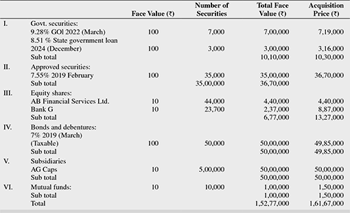
Note the following:
The bank classifies the entire government and approved securities into current investment category. The prices of government securities on the RBI list for sale are as follows:
| Security | Maturity | Sale price (`) |
|---|---|---|
| 5.25% | 2020 | 98.90 |
| 6.10% | 2022 | 102.25 |
For all other government securities (central and state), the following YTMs are applicable on 31 March, 2016.
| number of Years | YTM (%) |
|---|---|
| Less than 1 | 4.30 |
| 1 | 4.50 |
| 2 | 4.54 |
| 3 | 4.60 |
| 4 | 4.66 |
| 5 | 4.83 |
| 6 | 4.96 |
| 7 | 5.05 |
| 8 | 5.05 |
| 9 | 5.07 |
| 10 | 5.17 |
The shares of Bank G are traded in the market at ₹27. Since, AB Financial Services Ltd. is not a listed firm, the investment is valued, based on the latest audited accounts at ₹2.40 lakh.
For valuation of taxable bonds, 1 per cent above the applicable YTM rate is to be applied.
The net asset value (NAV) of the mutual fund is ₹10.75.
Provision made during the previous year stands at ₹18 1akh.
What would be the provision required to be made in respect of depreciation in investments during the current year?
Solution
The term to maturity of 9.28% GOI 2022 is 6 years and hence the corresponding YTM is 4.96 per cent from the table. We can use YTM formula33 to calculate the sale price of the security.

Similarly, YTM for 8.51 per cent state government loan for 9 years term to maturity is 5.07 per cent (the term to maturity of 8.9 years is rounded off to 9 years).

Similarly, the price for 7.55 per cent security maturing February 2019 is

Since AB Financial Services Ltd. is not a listed company, no market quote is available for it. The break up value of ₹2.40 lakh can, therefore, be assumed as the appropriate value. In the case of Bank G, the value would be 27.00 × 23700 = ₹6,39,900
The valuation of 7 per cent bonds maturing March 2019 (taxable) is as follows:
Term to maturity = 3 years
YTM = 4.60 + l.00% = 5.60%

Investments in the subsidiary, being permanent in nature, will be shown at book value.
Mutual funds are valued at current NAV.
Now, we can recast the investment schedule as follows:

Within an investment basket, appreciation is netted off against depreciation. However, the net depreciation is only considered and net appreciation is ignored. Thus, for the year the bank has to make a provision on the depreciated amount of `4,89,600 alone. (Baskets III + VI)
CHAPTER SUMMARY
- Typically, banks invest in securities to meet the following objectives: safety of capital, liquidity, yield, diversification of credit risk, managing interest rate risk exposure and meeting pledging requirements.
- Regulators stipulate that banks divide their security holdings into three categories based on the objectives of such investment like, held to maturity (HTM), held for trading (HFT), and available for sale (AFS).
- A bank’s ‘treasury’ is a source of substantial profit to the bank creating substantial value to shareholders. Banks’ treasuries typically perform the following basic functions within their investment and trading activities like, (a) investment advice and assistance to customers, including other banks, in order to manage their investment portfolios, (b) an important role in structuring products to hedge the bank’s own capital, (c) buying and selling securities on behalf of the customers and (d) as traders, also speculating on short-term interest rate movements.
- The treasury departments act as risk managers for banks. By using sophisticated internal transfer pricing, the treasury buys and sells funds among the bank’s client-facing units thus isolating and removing maturity and interest rate mismatches from corporate and retail business units. As markets develop, many credit products are being replaced by treasury products. An example is working capital credit being substituted by commercial paper.
- There are three important sources of treasury profit: (a) foreign exchange business, (b) money market products and (c) securities markets products.
- The primary objective of banks’ investment portfolio and treasury operations is to maximise earnings while mitigating risks involved. There are three predominant methods by which bank investments contribute to earnings: (a) interest income, (b) income from reinvestment, and (c) capital gains or losses.
- However, the earnings from investment are susceptible to the following risks: (a) interest rate risk, (b) credit risk in case the investment in debt securities does not yield the promised interest and principal payments, (c) liquidity risk that could arise from lack of market for the securities held and (d) other general risks that could cause volatility in returns from the investment portfolio, for example, inflation risk.
- Value at Risk (VaR) has become one of the standard measures to quantify market risk. VaR is defined as the maximum potential loss in the value of a portfolio due to adverse market movements for a given probability. VaR measures are used both for risk management and for regulatory purposes.
- However, the limitations of VaR are prompting regulators to look at alternative measures such as the Expected Shortfall (ES).
- In terms of the existing guidelines from the RBI, banks will have to hold their investments under either of the following categories – permanent or current investment. The permanent category will be held to maturity and are also called investment securities as they are held for the benefits of long-term yields. The current category comprises of dealing securities and is held in the trading book to take advantage of short-term fluctuations in prices.
- These investments will be valued based on the following guidelines: (a) HTM investments are to be carried at acquisition cost and need not be marked to market unless the market value exceeds the face value – any diminution, other than temporary, in the value of banks’ investments in subsidiaries/joint ventures should be provided for, (b) the individual securities in the AFS category will be marked to market at quarterly or at more frequent intervals. Net depreciation, if any, shall be provided for Net appreciation, if any, should be ignored. (Net depreciation is required to be provided for in any one category of securities (six broad categories defined) cannot be set off against net appreciation in any other category and (c) individual securities under the HFT category will be marked to market at monthly or more frequent intervals and provided for (as in the case of those ‘available for sale’).
TEST YOUR UNDERSTANDING
- Rapid fire questions
Answer ‘True’ or ‘False”
- Banks invest in securities with low default risk to preserve capital
- Market borrowings carry interest rate risk
- Higher returns will flow from investments with lower risk
- Market investments help diversify credit risk
- Bank treasury cannot give investment advice to customers or other banks
- Bank treasury can buy and sell securities on behalf of customers
- Banks cannot speculate in the financial markets
- Treasury profits are higher since operating costs are lower
- Treasury cannot deal with foreign exchange business of the bank
- Banks cannot invest in the equity markets
Check your score in Rapid fire questions
- True
- True
- False
- True
- False
- True
- False
- True
- False
- False
- Fill in the blanks with appropriate words and expressions
- Interest rate risk can lead to ————— volatility
- Banks have to divide their security holdings into three categories, depending on the ————— of the investments
- ————— securities are purchased by the bank with the objective of selling in the near term
- The treasury buys and sells funds internally among the business units of the bank by a process called —————
- The risk measure VaR is being replaced with the ————— method by the Basel Committee
- Expand the following abbreviations in the context of the Indian financial system
- HTM
- HFS
- AFT
- VaR
- ES
- NPI
- CP
- CD
- YTM
- BA
- Test your concepts and application
- Which of the following risks is present in a Repo transaction?
- Interest rate risk
- liquidity risk
- counter party risk
Substantiate your answer.
- 91 day T-bill of face value ₹100 is purchased at a yield of 5 per cent. What is the purchase price of the T-bill?
- Under which of the following circumstances should a bank rebalance its investment portfolio?
- a change in interest rates
- a change in the bank’s investment objectives
- a change in regulation
Substantiate your answer.
- How can banks assess the credit risk in their investment portfolio?
- How can banks use their investment portfolio to speculate on interest rate movements?
- What will be the VaR of a bond of 2 year maturity, whose price is `100 and whose yield and coupon are both at 5.8 per cent? The bank wants to hold the bond for one quarter. Assume that the annual standard deviation of 2 year treasury yields at 1.25 per cent and a confidence interval of (a) 95 per cent and (b) 99 per cent.
- Bank A has recently added the listed company DEF Ltd. to its investment portfolio. The bank bought 100 shares of DEF Ltd. at ₹400 per share with the intention of holding the shares for one quarter. The annual volatility of the stock is assessed at 25 per cent. If there are 250 trading days in a year, compute the VaR of the bank at 95 per cent confidence interval for the equity investment in DEF Ltd. over the holding period.
- VaR of ₹10 crore with 80 per cent confidence for bank A means –
- Bank A is 80 per cent certain that it will earn less than ₹10 crore
- Bank A’s investment portfolio will yield a return of at least 20 per cent
- Bank A is 80 per cent sure that it will not lose more than ₹10 crore
- There is a 20 per cent chance that Bank A will earn more than ₹10 crore on its portfolio
- What do you think will happen to the VaR of a portfolio when:
- The portfolio’s volatility increases
- The portfolio’s volatility decreases
- The portfolio’s average returns are higher
- The portfolio’s average returns are lower
- When the confidence level is increased
- When the confidence level is decreased
- When the holding period is increased
- When the holding period is decreased
- Which of the following risks is present in a Repo transaction?
TOPICS FOR FURTHER DISCUSSION
- The RBI website gives information on all banks. Study the investments patterns of banks in various categories – public sector, private sector and foreign. Do you notice any difference in their approach to investments? Has the approach been changing over time? What do you attribute the changes, if any, to?
- Study the current balance sheet of any bank in India, particularly its investment portfolio. Are there any risks that are inherent in the portfolio? Are there any potential risks that can arise in future?
- Did inappropriate VaR models mislead banks and contribute to the global financial crisis?
- How will the Expected Shortfall (ES) improve market risk management in banks?
SELECT REFERENCES
- Jorion, Philippe (2005). Access at http://www.gsm.uci.edu/~joriOfl/oc/CaSe.html
- Koch, Timothy and Scott S MacDonald. Bank Management, Chapter 19, 765–817, 4th ed. The Dryden Press.
- Linsmeier, Thomas J and Neil D Pearson (1996). Risk Measurement: An Introduction to Value at Risk. University of Illinois at Urbana-Champaign, July 1996.
- Lopez, Jose A (1997). “Regulatory Revaluation of Value-at-Risk Models”, Research Paper no. 9710, March, Federal Reserve Bank of New York. Managing Market Risk—Banks’ Investment Portfolio
ANNEXUREI
CASE STUDY—LTCM COLLAPSE AND LINK WITH VAR
In 1998, LTCM, the world’s largest hedge fund, failed and sent shock waves through the world’s financial system. LTCM’s size made the Federal Reserve Bank of New York step in to facilitate a bailout to the fund, fearing the negative impact of the liquidation on global financial markets.
It has been widely reported that the primary contributory factor to LTCM’s failure has been its poor risk management.
With a capital base of USD 3 million, LTCM possessed derivatives whose value exceeded USD 5 trillion and controlled over USD 100 billion in assets, globally – making it one of the most highly leveraged funds in the history. To predict and mitigate its risk exposures, LTCM used a combination of different VaR techniques and claimed that its VaR analysis showed that investors might experience a loss of 5 per cent or more in about 1 month in 5 and a loss of 10 per cent or more in about 1 month in 10. Only 1 year in 50 should it lose at least 20 per cent of its portfolio. LTCM also estimated that a 45 per cent drop in its equity value over the course of a month was a 10 standard deviation event. In other words, this scenario had no likelihood of occurrence (Prabhu, 2001). However, this ‘most unlikely’ event happened in August 1998. In spite of sophisticated hedging strategies, LTCM went wrong in one basic assumption – that historical trends in securities movements were an accurate predictor of future movements. The VaR models used by LTCM relied on historical data to predict future price movements. Unfortunately, the future holds too many uncertainties that the past cannot predict was the lesson learned by the management and investors at a very great cost.
For example, on 18 October 1987, 2 month S&P futures contracts fell by 29 per cent, which under the hypothesis of a lognormal distribution with annualized volatility of 20 per cent (which was also the approximate historical volatility of this security) would have denoted a 27 standard deviation event. Experts opined that the possibility of such an event happening would have been virtually impossible. Again, 13 October 1989 saw the S&P 500 fall about 6 per cent, a 5 standard deviation event under similar assumptions as above. Again, experts opined that such an event would have the likelihood of occurring only once in 14,756 years!
In August 1998, some unexpected events occurred, which were beyond the ‘predictive abilities’ of the VaR models used by LTCM. The Russian crisis triggered drying up of liquidity in the global financial markets and derivative positions were quickly slackened. Yet, LTCM’s VaR models continued to estimate that the daily loss would be no more than USD 50 million of capital. But the fund started losing around USD 100 million every day. On the fourth day in the wake of the Russian debacle, the fund lost USD 500 million in a single trading day.
While LTCM prepared to declare bankruptcy, the US Federal Reserve extended a USD 3.6 billion bailout to the fund, which was questioned by the experts who felt that such an action could create a moral hazard problem.
Hence, though perceived to be a highly effective risk measurement tool, VaR has to be used judiciously. At the end of August 1998, LTCM had USD 2.3 billion of equity capital and USD 1 billion excess liquidity. However, the firm was caught in a dilemma between reducing risk and raising additional capital. The magnitude of its positions rendered it unable to reduce its risk exposures immediately or attract new investors and it appeared that it had underestimated its capital needs. In retrospect, the fund was maximizing return while based on the simplistic assumption that volatility would remain constant, while in reality it could easily double in turbulent times.
The fund was not able to liquidate quickly enough in case of adverse market conditions, leading to a risk of liquidity and insolvency. Liquidity risk is not factored into VaR models since they assume that normal market conditions will prevail.
Therefore, it appears that LTCM’s actual exposure to liquidity and solvency risks was not adequately exposed by its VaR model.
While VaR is seen as an invaluable tool to measure risks, complementary measures such as, stress testing could have probably offset the limitations and disadvantages of VaR While VaR could show fund managers what they could lose with a predetermined maximum probability, stress tests enable them to assess their possible loss if the worst case scenario materialized.
The case of LTCM serves to illustrate the practical dimensions of a popular risk measurement instrument like the VaR.
QUESTIONS ON THE CASE STUDY:
- LTCM failed due to bad strategy, bad execution or bad luck?
- If VaR were a flawed model, why was it so widely used?
- Is Expected Shortfall (ES) an improvement over VaR? What are the issues with ES?
SELECT REFERENCES
- Feridun, Mete (2005). “Value at Risk: Any Lessons from the Crash of Long Term Capital Management (LTCM)?”. Journal of Business Administration Online, Spring 2005, vol. 4, no. 1. http://jbao.atu.edu.
- Prabhu, Siddharth (2001). “Long Term Capital Management: The Dangers of Leverage”. Duke University, Durham, May 2001.
ANNEXURE II
SUMMARY OF REGULATORY RESPONSES TO MARKET RISK MEASUREMENT PRACTICES BY BANKS AFTER THE GLOBAL FINANCIAL CRISIS
A series of bank failures in the 1970s prompted the setting up of the Basel Committee on Banking Supervision, with the intention to regulate financial institutions, particularly banks. A detailed discussion on the Basel Committee has been carried out in another chapter in this book.
Since its inception, the Committee has focused on regulation of bank capital globally. The measure of capital is based on the asset portfolio risks individual banks take, as well as operational risks in banking operations. An important part of the asset portfolio risk is ‘market risk’ caused by adverse fluctuations in market factors. The risk measure agreed upon for market risk measurement was the VaR.
Significant weaknesses were identified in the Basel II framework for trading activities, and the framework has taken its share of criticism for the global financial crisis of 2007-08. To address the most conspicuous deficiencies in the framework, the Basel committee introduced a set of revisions to the Market risk framework in 2009 – termed the Basel 2.5 package of reforms. A further process to fine tune and redesign the capital standard for market risk was undertaken.
Basel 2.5 required banks to hold additional capital for default and ratings migration risk, that is, the risk that a rating change in the market instrument triggers significant mark-to-market losses. Banks were also asked to calculate an additional VaR capital charge, called the “Stressed VaR”. The new framework also brought in changes in the treatment of securitization exposures. However, Basel 2.5 was seen to not address all the structural shortcomings with the market risk framework.
The Basel Committee has since published three consultative documents on the trading book review: Fundamental review of the trading book, May 2012, www.bis.org/publ/bcbs219.htm; Fundamental review of the trading book: A revised market risk framework, October 2013, www.bis.org/publ/bcbs265.htm; and Fundamental review of the trading book: Outstanding issues, December 2014, www.bis.org/bcbs/publ/d305.htm
The final rule on the Fundamental Review of the Trading Book (FRTB) was published in January, 2016, called the “Minimum Capital requirements for market risk” (http://www.bis.org/bcbs/publ/d352.pdf), after five years of discussion, four Quantitative Impact Studies (QIS), and three consultative papers.
The final rule is being commonly referred to as ‘Basel 3.5’ or ‘Basel 4’, since it is considered the first of many rules related to Basel 4 that are anticipated to be finalized soon, and is expected to have significant impact on trading book definition, risk measurement, assessment and reporting at financial institutions all over the world.
Figure 10.1 summarizes the key aspects of the FRTB
FIGURE 10.1 FRTB AND THE MARKET RISK FRAMEWORK – A BIRD’S EYE VIEW

Banks are required to report under the new standards by end of the year 2019.
FRTB at a Glance
- New rules determining the scope of instruments eligible for inclusion in the trading book, and more stringent requirements governing internal risk transfers between the banking and trading book.
- A revised standardised approach for market risk based on price sensitivities, which is intended to be more risk sensitive compared to the existing standard approach, and therefore reduce the gap between internal models and standard rules.
- The substitution of value at risk and stressed value at risk with an expected shortfall risk measure to capitalise for loss events in the tail of the P&L distribution.
- The introduction of liquidity horizons in the expected shortfall calculation to reflect the period of time required to sell or hedge a given position during a period of stress.
- Replacement of the incremental risk charge with an incremental default risk model, which is designed to capture default risk in the market risk framework.
- Back-testing requirements of internal models at trading desk level. Failure to meet the validation criteria would force a desk to revert to using the standardised approach.
- Enhanced public disclosures on market risk capital charges, including regulatory capital charges calculated using both standardised and internal models approaches.
Estimating ES under the FRTB rules
Under the rules, Stressed Expected Shortfall is to be calculated at the 97.5th percentile for each trading desk (as specified in the Basel committee document quoted above). Appropriate “Liquidity horizons” are to be used for scaling up the ES from the base horizon. This will pose a challenge to banks, especially in the areas of data gathering and analytics and model building.
ENDNOTES
- ‘Unrealized’ since the gain or loss would crystalise only if the bank decides to sell the bond in the market at that value.
- Both the terms ‘money market’ and ‘commercial paper’ are being explained subsequently in this chapter.
- More discussion on these products will be found in the chapter on ‘International Banking’.
- The bank stamps the word ‘accepted’ on the face of the instrument.
- Letters of credit (LCs) are documents governed by the rules of the International Chamber of Commerce (ICC). These documents stipulate contract terms and duties of parties to the LC (the importer, exporter and the participating banks) and authorizes the exporter to draw a draft on a participating bank for payment to be received from the importer.
- ‘Investment grade’ implies bonds that are likely to meet all payment obligations on time. According to Moody’s, Aaa, Aa, A and Baa signify investment grade ratings, while according to Standard and Poor’s, AAA, AA, A and BBB constitute investment grade ratings. For more on Credit Ratings, please refer earlier chapters on credit.
- ‘Zero coupon’ implies that the bond does not pay periodic interest. Hence, the bond is sold at a discount from the face value.
- Defined in the previous chapter. To recap, ‘passthroughs’ constitute a pool of fixed income securities backed by a package of assets. A servicing intermediary collects the monthly payments from issuers and after deducting a fee, remits or passes them through to the holders of the pass-throughs. They are also known as a ‘pass-through security’ or ‘pay through security’. The most common type of pass-through is a mortgagebacked certificate where homeowners’ payments pass from the original bank through a government agency or investment bank to investors.
- These and other securitized instruments were considered to be one of the leading causes of the global financial crisis. For a detailed discussion on the instruments and the crisis, please see chapters related to Credit.
- Convertible bonds are a mix of debt and equity, where the bond holders are given the option to convert debt into equity on a predetermined date at a predetermined price.
- The explanation for this is as follows: Bond value is measured as
 where i = 1 to n years, C is the coupon rate, n is the number of years to maturity, r is the periodic required return, M is the maturity value, and i the time period when payment is received. If the interest rate falls during this period, investors start expecting less. Since the denominator would now decrease, the bond value would increase. If interest rates rise during this period, the reverse would happen and the bond value would decrease.
 - ‘Investment grade’ are those securities rated in one of their four highest ratings by nationally/internationally recognized external rating agencies such as Standard & Poor or Moody’s.
- More on the Basel Committee in Chapter, ‘Capital – Risk, Regulation and Adequacy’.
- In particular, please refer to Mandelbrot, B, (1963), ‘The variations of certain speculative prices’, Journal of Business 36, 394–419, and Fama, E, (1965), ‘The behavior of stock market prices’, Journal of Business 38, 34–105.
- Manganelli, Simone, and Robert Engle, (2001), ‘Value at risk models in finance’, European Central Bank Working Paper no 75, August 2001. Page 7.
- ‘Covariance’ is a statistical concept that measures how two or more assets move in tandem. A positive covariance signifies that the asset returns move together and a negative covariance moves inversely. Hence, the ‘correlation’ between two assets can be expressed as the covariance between the two assets divided by the product of the standard deviation (volatility) of the two assets.
- ‘Risk Metrics sells its VAR modeling and other services to 3,500 institutions, including the world’s top ten investment banks and 70 of its 100 largest money managers. It also provides small investors free access to quick-and-dirty ways to X-ray their own holdings’ (appearing in Forbes magazine, 13 October 2008, accessed at http://www.forbes.com/forbes/2008/1013/060.html on June 5, 2009).
- Detailed description of the methodology can be found in ‘Risk MetricsTM – Technical document’, J.P. Morgan/ Reuters, 4th edition, December 1996, ‘Return to Risk Metrics: The Evolution of a Standard’, Risk Metrics Group Inc., April 2001, and ‘The Risk Metrics 2006 Methodology’, Zimbach, Gilles, Risk Metrics Group, March 2007, all accessed at www.riskmetrics.com
- Bollerslev, Tim. (1986), ‘Generalized Autoregressive Conditional Heteroskedasticity’, Journal of Econometrics, 31, pp. 307–27, and Engle, Robert F.(1982) ‘Autoregressive Conditional Heteroskedasticity with Estimates of the Variance of U.K. Inflation’, Econometrica, 50, pp. 987–1008. The term ‘heteroskedasticity’ signifies ‘different variances’;, and more details can be found in statistics textbooks.
- GARCH stands for ‘generalized auto regressive conditional heteroskedasticity’, and is a generalization of Engle’s (1982) ARCH model, used to model financial time series that exhibit time variable volatility clustering – for example, periods of wild fluctuations followed by periods of relative calm. GARCH uses autoregressive moving averages.
- Boudoukh, Jacob, Mathew Richardson and Robert Whitelaw,(1998), ‘The best of both worlds’, RISK 11, 64–67.
- Verma, Jayanth R, (2009), ‘Risk management lessons from the global financial crisis for derivative exchanges’, Working paper no. 2009-02-06, Indian Institute of Management, Ahmedabad.
- (http://www.risk.net/riskmanagement/marketrisk/2375185/hullandwhiteontheprosandconsofexpectedshortfall)
- RBI Master Circular–Prudential norms for classification, valuation and operation of investment portfolio by banks, July 1, 2015.
- Ibid., Page 4
- Statutory Liquidity Ratio. Please see Chapter ‘Monetary Policy – Implications for Bank Management.’
- All bank balance sheets should present the investment portfolio with the six classifications. We have seen this when we studied the financial statements of banks in India – refer Chapter ‘Banks’ financial statements’.
- See Chapter ‘Monetary Policy Implication for Bank Management’ for composition of DTL.
- Primary (PD) dealers are commercial banks or brokers/ dealers authorized to buy and sell government securities, subject to minimum capital requirements.
- The Fixed Income Money Market and Derivatives Association of India (FIMMDA), an association of commercial banks, financial institutions and primary dealers was incorporated as a company under section 25 of the Companies Act, 1956 on 3 June 1998. F1MMDA is a voluntary market body for the bond, money and derivatives markets. It has members representing all major institutional segments of the market. The membership includes State Bank of India and its associates, nationalized banks, private sector banks, foreign banks, financial institutions and all primary dealers.
- YTM – Yield to Maturity. Academically YTM is defined as the market interest rate that equates a bond’s present value of interest payments and principal repayment with its price. YTM can also be defined as the compound rate of return that investors will receive for a bond with a maturity greater than one year if they hold the bond to maturity and reinvest all cash flows at the same rate of interest. It takes into account purchase price, redemption value, coupon yield and the time between interest payments. The YTM is easy to compute where the acquisition cost of a bond is at par and coupon payments are effected annually. In such a situation, the yield to maturity will be equal to coupon payment. However, for other cases, an approximate YTM can be found by using a bond yield table. In the absence of taxes, YTM would be an accurate measure of return if the yield curve were flat and interest rates remained constant over the life of the bond. It becomes a poorer measure as the yield curve becomes steeper or as the purchase price deviates further from par.
- For more details on securitization/reconstruction companies, please refer chapter, ‘Credit Risk—An Overview’.
- Typically, YTM is calculated either by discounting the cash flows over the period remaining till maturity or by an approximation which equates the YTM to (1 + (F- P)/n)/(0.4F + 0.6P), where I denotes the interest rate, F the face value, P the market price and n the term to maturity.
- Calculated from the YTM formula given above.