
CHAPTER TWELVE
Managing Interest Rate and Liquidity Risks
CHAPTER STRUCTURE
Section I The Changing Face of Banking Risks
Section II Asset Liability Management
Section III Interest Rate Risk Management
Section IV Managing Interest Rate Risk with Interest Rate Derivatives
Section V Liquidity Risk Management and Basel III
Section VI Applicability to Banks in India
Annexures I, II, III, IV, V, VI (Case study)
KEY TAKEAWAYS FROM THE CHAPTER
- Understand why risk management is important for banks.
- Understand sources of asset liability risk, interest rate risk and liquidity risk.
- Learn how interest rate risk is managed.
- Learn how interest rate derivatives work.
- Learn how liquidity can be managed.
- Understand the International and Indian standards for measuring and managing interest rate and liquidity risks in banks.
“The business of banking is the business of risk management; plain and simple, that is business of banking.”
—Walter Wriston, Ex CEO, Citibank
SECTION I
THE CHANGING FACE OF BANKING RISKS
Consider a bank that borrows ₹100 crores at 5 per cent for a year, and lends the money at 5.5 per cent to a highly rated borrower for 5 years. For simplicity, let us assume interest rates are to remain fixed over the period of the loan; they are annually compounded and all interest accumulates to the maturity of the respective obligations. The net transaction appears profitable since the bank is earning a 50 basis point spread.
But the transaction is not without risks.
- At the end of a year, the bank will have to repay ₹100 crores to the depositor(s), and find new sources of financing for the loan, which still has 4 years to maturity. If the bank is not able to find sources for repayment, it runs a ‘liquidity’ risk, which could threaten the ‘solvency’ of the bank.
- At the end of the year, if interest rates have risen, the bank would have to pay a higher rate of interest on the new financing, thus narrowing the spread. Suppose, at the end of a year, an applicable 4-year interest rate is 6 per cent. The bank is in trouble. It is going to earn 5.5 per cent on its loan and pay 6 per cent on its financing. In short, the bank will be losing money on this transaction! Thus, the transaction has also entailed an ‘interest rate’ risk for the bank, which would impact the bank’s net income
Also consider the following scenarios:
- Ninety per cent of Bank A’s liabilities mature within the next 12 months. Bank A has invested 80 per cent of these funds in securities maturing after 5 years.
- Ninety per cent of Bank B’s liabilities mature within the next 12 months. Bank B lends 75 per cent of these funds to various infrastructure projects, where the repayments will start after an initial payment holiday of 2 years.
- Eighty per cent of Bank C’s liabilities mature after 3 years and have been borrowed at fixed cost. Interest rates are on a downward trend, and 80 per cent of Bank C’s loan portfolio consists of short-term loans to be fully repaid over the next 6 months.
- Bank D has entered into dollar forward contracts at a premium for 6 months on behalf of its importer borrowers, who form about 60 per cent of the bank’s loan portfolio. There is a fall in dollar value during this period.
What are the potential dangers in each of the above scenarios?
In the first two scenarios, the banks face a liquidity risk. When the liability holders demand their money in the next 12 months, the banks may not have enough cash to repay them, since the cash flow from the assets would be delayed beyond this period. In the third scenario, Bank C faces an interest rate risk. The short-term loans would be repaid, and the cash inflow will have to be lent by the bank at the prevailing lower rates, while the bank will have to continue paying interest on liabilities at the original contract rates till they mature. The bank’s spreads would narrow further and impact the net earnings. Bank D, evidently, faces an exchange rate risk.
The primary problem in these examples was a ‘mismatch’ between the bank’s assets and liabilities. Prior to the 1970s, many firms in developed countries intentionally mismatched their balance sheets, and borrowed short and lent long to earn a spread, taking advantage of the upward sloping yield curves. Interest rates in developed countries experienced only modest fluctuations, so losses, if any, due to asset-liability mismatches were trivial.
Things started to change in the 1970s, which ushered in a period of volatile interest rates that continued into the early 1980s. The 1980s and 1990s also saw a new wave of banking crises in the developed world and emerging markets. These events challenged the traditional view that ‘runs’ on solvent banks were at the heart of banking panics and that panics were the main causes for banking crises. The striking fact here was that ‘bank runs’ had played a negligible role in most of these events.
With new financial instruments such as derivatives, new participants such as hedge funds and new technologies such as e-banking, the informational efficiency of markets to match savings with investment opportunities improved substantially in the early years of the 21st century.
The growth in derivatives markets has no doubt increased the tools available to firms to take on and manage risks, but has also made risk exposure assessment tougher for regulators, as the financial crisis of 2007 has amply demonstrated. For example, a bank can take large risks through trading of derivatives, without making the exposure visible on its balance sheet. Traditionally, banks exposed themselves to interest rate risks by taking deposits, making loans or buying securities. With derivatives, banks can use swaps to take on the same interest rate risk as, say, in the case of buying bonds. However, the swaps are not recorded on the banks’ balance sheets because the value of swaps at inception is typically zero. After inception of the swap, mark-to-market accounting requires the banks to record the market value of the swap, but that market value provides little indication of the magnitude of banks’ interest rate exposure.
Moreover, banks could improve their traditional ‘return on equity’ measure through taking on risks for feebased activities, without capital outlay.
Such developments have forced bank regulators and market participants to look for risk management approaches that would go beyond mere accounting numbers to capture realistic assessments of adverse outcomes, and reveal the actual risks borne by financial institutions. Figure 12.1 illustrates the sources of banking risks.

From Figure 12.1 and our discussions in earlier chapters, it is evident that banks are subject to various interdependent risks. Though, for convenience of measurement and analysis we isolate them, in reality, what starts off, say as a credit risk event, can snowball into a bundle of other risks as well. For the same reason, it appears difficult to conclude about the overwhelming cause of the financial crisis of 2007—was it subprime lending practices, or financial instruments, such as the Credit Default Swap or CDOs, or was it transactions such as securitization, or was it excesses in human greed and negligence?
However, one inference is clear—all banks and financial institutions will have to undertake a profound revision of their approach to risk management.
A relook at risk management does not imply that banks scale down their risk appetite, which is essential for future progress and survival in a competitive and developing environment. The implication only highlights the need for banks to state their risk policies more clearly and stringently, and ensure strict adherence to the policies and safeguards.
To complement the published work of a number of eminent bodies on the financial crisis of 2007, a unique private sector initiative termed the Counter party Risk Management Policy Group III (CRMPG III) was formed in April 2008, chaired by top bankers from HSBC and Goldman Sachs.1 The Policy Group members are drawn from various leading multinational banks. The scope of this initiative was designed to focus primarily on the steps that the private sector should take to avoid future financial shocks.
The Policy Group identifies some common features characterizing the post 1980 financial crises—(a) credit concentrations, (b) broad-based maturity mismatches, (c) excessive leverage, and (d) the illusion of market liquidity. It also includes a ‘wild card’ in the form of macroeconomic imbalances. Overarching all these factors is collective human behaviour, where financial institutions tend to take on disproportionate risks on the upside of business or financial market cycles, and pull back fiercely when the cycle is on the downturn. In this context, the Group recognizes the need for private initiative to ably complement supervisory oversight to mitigate banking risks.
The Group has developed ‘core precepts’ to provide the broad framework for risk management in banks that focus on the basics of (a) corporate governance, (b) risk monitoring, (c) estimating risk appetite, (d) contagion effects, and (e) enhanced oversight. The salient features of the recommendations in respect of these precepts call for the highest quality of risk management and governance within the bank, and supervision by external administrators.
We have discussed credit, market and operational risks in earlier chapters. In the following sections of this chapter, we will discuss the ‘wild card’ risk that broadly translates into interest rate risk, and most important, liquidity risk, a product of the various factors listed above.
SECTION II
ASSET LIABILITY MANAGEMENT
Risk management is uniquely important for financial institutions because, in contrast to firms in other industries, their liabilities are a source of wealth creation for their shareholders.2
Over the years, banks have been focusing on ‘asset-liability risk’ to mitigate balance sheet weaknesses. The problem is not that the market value of assets might fall or that the value of liabilities might rise. It is that capital might be depleted by narrowing of the difference between assets and liabilities, since the values of assets and liabilities may not always move together, in the same direction. Asset-liability risk, therefore, is a ‘leveraged’ risk. As we have already seen, the capital of banks is small relative to the firm’s assets or liabilities, so small percentage changes in assets or liabilities can translate into large percentage changes in capital.
The Asset-liability risk described above could manifest itself in more than one form, but what would concern bankers most would be two important risks—‘interest rate’ risk and ‘liquidity’ risk. While interest rate risk would directly impact the net income of the bank, the liquidity risk would endanger the very solvency of the bank.
The above need for risk management led to the evolution of Asset-liability management (ALM) in the 1980s. In a way, ALM was seen to substitute for market-value accounting3 in a context of accrual (book value) accounting. Traditionally, banks and insurance companies have been using accrual accounting for essentially all their assets and liabilities. They would take on liabilities, such as deposits, life insurance policies or annuities. They would invest the proceeds from these liabilities in assets such as loans, bonds or real estate. All assets and liabilities were held at book values. Doing so did not recognize the possible risks arising from how the assets and liabilities were structured, or how the markets were moving. To overcome these shortcomings, a combination of ALM and market value accounting was advocated.
However, many of the assets and liabilities of financial institutions cannot be marked to market. A firm can earn significant mark-to-market profits but go bankrupt due to inadequate cash flow. Market-value accounting was therefore not the ideal solution.
However, where found suitable, banks are increasingly using market-value accounting for certain business lines. This is true of universal banks with trading operations, which find techniques of market risk management such as Value at Risk (VaR),4 market risk limits, etc. more appropriate. On the other hand, ALM is associated with those assets and liabilities—those business lines—that are accounted for on an accrual basis. This includes bank lending and deposit taking.
In short, ALM is concerned with strategic balance sheet management. Risks caused by changes in interest rates and exchange rates, credit risk and the bank’s liquidity position have to be monitored and mitigated. With profitability of banking operations and the long-term solvency of banks becoming key factors, it has now become imperative for banks to move away from partial asset management (credit, non-performing assets) and partial liability management (deposits) to integrated balance sheet management. In such an approach, all components of a bank’s balance sheet, their maturity mix, their pricing and risks will be looked at not only from the angle of profitability, but also from the angle of solvency and long-term sustenance.
Techniques of ALM have been evolving over time. Banks typically have an Asset Liability Management Committee (ALCO) that comprises of a group of top or senior management personnel entrusted with the responsibility of managing the bank’s assets and liabilities to balance the various risk exposures, to enable the bank achieve its operating objectives.
Table 12.1 depicts the shift from traditional ALM objectives and practices to modern ALM techniques.
TABLE 12.15 TRADITIONAL ALM OBJECTIVES AND PRACTICES TO MODERN ALM TECHNIQUES

At present, in almost all banks, ALCO has the responsibility to devise broad strategies for handling banks’ competing long-term needs, and also monitor and manage interrelated risk exposures on a daily basis. Therefore, the ALCO of a bank is the focal point for coordinating the bank’s diverse activities to accomplish its operating objectives. Towards this objective, the ALCO receives and analyzes a wide variety of reports that bring together information on the bank’s asset/liability positions, its capital level, its internal plans and current and projected external conditions. Some typical types of information and analyzes the ALCO might receive include (a) information on current and projected national and local economic conditions, (b) interest rate forecasts, (c) current loan and deposit positions, showing the asset and liability mix, highlighting concentrated exposures, (d) forecasts of cash inflows and outflows on account of assets and liabilities, based on commitments and likely trends, (e) the current and projected liquidity position for the bank, and (f) an analysis of the potential effects of interest rate risk on the bank’s income and capital position.
Most ALCOs primarily focus on managing the bank’s liquidity and interest rate risks, while a separate committee would be involved in managing credit risks. In practice, evaluating interest rate and liquidity risks involve the consideration of different possible scenarios. For example:
- What if the bank experiences an unexpectedly large volume of deposit withdrawals?
- What if loan repayments occur earlier than anticipated? Or later than due date? Or not at all?
- What happens if interest rates suddenly rise by x basis points?
- What happens if counterparties do not keep up commitments? Or off-balance sheet items turn into real cash outflows?
The ALCO’s challenge is to assess the probability with which similar events would occur, and position the bank to handle the most likely scenarios with the minimum impact on the bank’s expected performance and solvency.
The ALCO will therefore operate with the objectives of (a) assessing the probability of various liquidity shocks, (b) assessing the probability of various interest rate scenarios and their impact on the bank’s net income, (c) positioning the bank to handle the most likely of these scenarios at minimum cost (impact on net income and the bank’s capital), while achieving a reasonable profitability level, and (d) allocating the bank’s remaining assets and liabilities to meet risk and profitability objectives.
ALM departments also handle foreign exchange and other risks. The growth of derivatives markets helped in ALM by facilitating a variety of hedging strategies, while securitization allowed banks to directly address assetliability risk by removing assets from their balance sheets.
Of the important risks that ALM addresses, interest rate risk and liquidity risk are accorded paramount importance. We shall study these in detail in the following sections.
SECTION III
INTEREST RATE RISK MANAGEMENT
Simply stated, interest rate risk is the exposure of a bank’s financial condition to adverse movements in interest rates. If accepted and managed as a normal part of banking business, interest rate risk can be used to enhance profitability and shareholder value. However, excessive interest rate risk could lead to substantial volatility in earnings and thus also affect the underlying value of the bank’s assets, liabilities and off-balance sheet instruments. Hence, an effective risk management process that aims at sound financial health of a bank would have to maintain interest rate risk within prudent levels. The two most common perspectives for assessing a bank’s interest rate risk exposure are (a) the earnings perspective that focuses on short-term earnings, and (b) the economic value perspective that looks at the long-term economic viability of the bank
Why are two approaches necessary? The ‘earnings perspective’ assesses the impact of changes in interest rates on the ‘net interest income’ (NII) (difference between total interest earned from loans and investments and total interest paid on deposits and borrowings) of the bank. This is the traditional method of risk assessment since reduced net interest earnings could threaten the financial stability of the bank and also impair market confidence. However, banks have been able to generate non-interest income from fee-based activities, such as loan servicing, transaction processing, off-balance sheet transactions or managing securitization pools, most of which depend on the way credit markets perform. Hence, a major portion of the fee-based income could also be interest rate sensitive, and banks would have to look at the impact of interest rate variations on net income as well.
‘Value’ or ‘economic value’ generally represents the present value of expected future net cash flows, discounted at appropriate market rates. For a bank, expected net cash flows would arise as the difference between expected cash flows on assets and the expected cash flows on liabilities, plus the expected net cash flows arising from off-balance sheet activities. We have seen earlier how variations in market interest rates can impact the economic value of banking assets, liabilities and off-balance sheet positions (contingent liabilities). Thus, the sensitivity of a bank’s economic value to fluctuations in interest rates is of great importance to all stakeholders—investors, management and supervisors—since it reflects the sensitivity of the bank’s ‘net worth’ to changes in interest rates. It is evident that the economic value perspective is more comprehensive and long term than the earnings perspective, since it considers the potential impact of interest rate fluctuations on future cash flows. This long-term perspective is valuable since short-term changes in earnings of a bank, which is the focus of the earnings perspective, cannot indicate realistically the impact of interest rate movements on the bank’s overall positions, and hence, its financial health in the long run.
But it is not always future interest rates that impact a bank’s financial performance. Past interest rates also have a continuing impact on future performance. For example, a long term, fixed-rate loan contract (as in the example quoted at the beginning of this chapter) may have to be refinanced at higher interest rates over the tenor of the loan. Securities not marked to market may contain embedded gains or losses due to past rate movements, which would be reflected over time in the bank’s earnings. Hence, the impact of such ‘embedded’ losses or gains due to past interest rates would also have to be assessed realistically.
Assessment of the extent of a bank’s interest rate risk by any of the perspectives given above would not be a simple exercise. Every asset on the bank’s balance sheet has different risk and return characteristics, different possible sources, repricing6 periods and so on. Box 12.1 presents some of the common sources of interest rate risk. The exercise would be rendered more complex by the discretion that the bank can exercise in adjusting the rates on assets and liabilities, or the likelihood of a change in bank customer behaviour (early repayment of loans or withdrawal of deposits) due to changes in market rates, or the interest rate sensitivity of fee-based income (non-interest income) and off-balance sheet exposures. In practice, banks will generally have a mix of all types of interest rate risk, with the effects potentially offsetting or reinforcing one another. It is the complexity of the resulting combination of factors that makes interest rate risk difficult to manage.
BOX 12.1 SOURCES OF INTEREST RATE RISK
As financial intermediaries, banks encounter interest rate risks arising from several factors fundamental to the business of banking. Some of the most discussed sources of interest rate risk are given as follows:
- Repricing risk: The primary and frequently discussed form of interest rate risk arises when the average yield on a bank’s assets or the average cost of its liabilities is more sensitive to changes in market interest rates. The difference in sensitivity could arise from possible mismatches in the asset and liability characteristics of the bank. First, fixed rate assets and liabilities could have different maturities. Second, floating rate assets and liabilities could have different repricing periods, with different base rates. For example, assets could reprice annually based on a 1-year rate and liabilities could reprice quarterly based on a 3-month base rate. Third, floating rate assets and liabilities could have base rates of different maturities, such as assets that reprice annually based on a long-term rate and liabilities that reprice annually based on a 1-year rate. Fourth, in countries with deregulated interest rates, banks can adjust pricing at will, and the rate-setting policies that banks follow determine the effective repricing behaviour of such instruments. The pricing decisions in these cases would then depend on a variety of factors in addition to market interest rates, such as the expected behaviour of bank customers and the extent of competition in the markets concerned. Finally, in some cases, bank customers have the option either to repay loans or withdraw their deposits at low (or no) cost, and the decisions of such customers would influence the response of the average pricing of such assets or liabilities to changes in market interest rates. Such repricing mismatches, though inherent to the business of banking, can expose a bank’s income and underlying economic value to unanticipated fluctuations as interest rates vary. For instance, a bank that funded a long-term fixed-rate loan with a short-term deposit could face a decline in both the future income arising from the position and its underlying value if interest rates increase. These declines arise because the cash flows on the loan are fixed over its lifetime, while the interest paid on the funding is variable, and increases after the short-term deposit matures.
- Yield curve risk: Even if, on an average, the yields on a bank’s assets and liabilities adjust to changes in market rates to the same extent, a bank may still be subject to yield curve risk. Yield curve risk is the possibility that changes in the shape of the yield curve7 could have differential effects on the bank’s assets and liabilities. For example, if a bank’s assets and liabilities reprice annually, it might want to balance a medium-term base rate for its assets with a mixture of short-term and long-term base rates for its liabilities. In that case, increased curvature of the yield curve would boost medium-term yields relative to short- and long-term yields, and thus raise the rate on the bank’s assets relative to the average cost of its liabilities, and reduce short-term earnings volatility.
Repricing mismatches can also expose a bank to changes in the slope and shape of the yield curve. Yield curve risk arises when unanticipated shifts of the yield curve have adverse effects on a bank’s income or underlying economic value. Annexure I provides an overview of the theory of interest rates, to enable understand the concept of yield curves.
- Basis risk: If the instruments have different base rates, the bank will be subject to basis risk. For example, yields on a bank’s floating rate assets could be tied to government security yields, while those on its floating rate liabilities could be based on an interbank rate such as the Libor. There is a possibility that the two base rates will diverge unexpectedly owing to differing credit risk or liquidity characteristics, which might increase private yields relative to government yields. In that case, the cost of bank liabilities would increase, relative to the yield on assets, thus lowering the bank’s earnings.
- Optionality: An increasingly important source of interest rate risk arises from the options embedded in many bank assets, liabilities, and off-balance sheet portfolios. Simply stated, an option provides the holder the right, but not the obligation, to buy, sell, or in some manner alter the cash flow of an instrument or financial contract. Options may be stand-alone such as exchange-traded options and over-the-counter (OTC) contracts, or may be embedded within otherwise standard instruments. While banks use exchange-traded and OTC options in both trading and non-trading accounts, instruments with embedded options are generally more important in non-trading activities. For example, bonds/securities may include options. Call options are typically exercised by the issuers to redeem bonds before maturity, while put options are exercised by investors to seek redemption before maturity. Such options could expose banks to interest rate risk. For example, if call option on the bonds are exercised when interest rates are declining, the bank investing in these bonds would run a ‘reinvestment risk’, since the intermediate cash flows from bond redemption would have to be reinvested at a lower rate. If, on the other hand, the bank has issued bonds with a put option, and interest rates are rising, the bank would face a ‘prepayment risk’ when investors seek redemption before maturity. The bank, in such cases, may have to borrow from the market at higher rates to pay the bondholders. Both these options, therefore, would cause earnings volatility for the bank.
Other examples of instruments with embedded options would be loans that give borrowers the right to prepay balances, or transaction deposit instruments that give depositors the right to withdraw funds at any time, often without any penalties.
If not adequately managed, the asymmetrical payoff characteristics of instruments with optionality features can pose significant risk particularly to those who sell them, since the options held, both explicit and embedded, are generally exercised to the advantage of the holder and the disadvantage of the seller. Moreover, an increasing array of options can involve significant leverage which can magnify the influences (both negative and positive) of option positions on the financial condition of the firm.
- Other sources of risk: Banks may also be subject to interest rate risk through interest sensitivity of their non-interest income. For example, lower interest rates could lead to prepayments (with the intention of refinancing the loans) that deplete the pool of loans serviced by a bank, thereby reducing its fee income, and also leading to a ‘prepayment’ risk. In a declining interest rate scenario, the cash inflows from prepayments could be invested only at lower rates, thus leading to more earnings volatility. More significant would be the substantial interest rate exposures embedded in the off-balance sheet positions of large banks, held either as a hedge for their on-balance sheet interest rate exposures or as a result of their trading activity in derivatives markets.
In order to understand interest rate risk, one has to understand the nature of interest rates. The management of interest rate risk depends substantially on predicting how interest rates would behave in future. If interest rates can be forecasted with a great deal of accuracy, interest rate risk is mitigated to a very large extent. Predicting future interest rates essentially involves predicting the shape of the future ‘yield curve’. Annexure I provides an overview of the various theories of interest rates, and how they could be used in predicting interest rate movements.
Interest rate risk in the banking book – Basel committee standards – Salient features
(Source: The Basel Committee on Banking Supervision, April 2016, “Standards : Interest rate risk in the Banking Book (IRRBB)” (http://www.bis.org/bcbs/publ/d368.pdf).
The concepts embodied in the foregoing part of this section is reflected in the current Basel committee standards on interest rate risk, its measurement and management.
In the global scenario following the financial crisis of 2007, interest rates in many countries are at very low levels, with some countries staring at negative interest rates. When interest rates normalize in the future banks in these countries would face a significant interest-rate risk.
IRRBB refers to the current or prospective risk to a bank’s capital and to its earnings, arising from the impact of adverse movements in interest rates on its banking book.
When interest rates change, the present value and timing of future cash flows change. This in turn changes the underlying value of a bank’s assets, liabilities and off-balance sheet items and hence its economic value (EVE). Changes in interest rates also affect a bank’s earnings by altering interest rate-sensitive income and expenses, affecting its net interest income (NII). Excessive IRRBB can pose a significant threat to a bank’s current capital base and/or future earnings if not managed appropriately.
The document includes the revised Principles, which replace the 2004 IRR (Interest Rate Risk) Principles for defining supervisory expectations on the management of IRRBB. Banks are expected to implement the revised standards by 2018. (Banks whose financial year ends on 31 December would have to provide the disclosure in 2018, based on information as of 31 December 2017.)
Types of risks
The Basel document identifies three main sub-types of interest rate risk. It is noteworthy that all three sub-types of IRRBB potentially change the price/value or earnings/costs of interest rate sensitive assets, liabilities and/or off-balance sheet items in a way, or at a time, that can adversely affect a bank’s financial condition
- Gap risk arises from the term structure of banking book instruments, and describes the risk arising from the timing of instruments’ rate changes. The extent of gap risk depends on whether changes to the term structure of interest rates occur consistently across the yield curve (parallel risk) or differentially by period (non-parallel risk).
- Basis risk describes the impact of relative changes in interest rates for financial instruments that have similar tenors but are priced using different interest rate indices.
- Option risk arises from option derivative positions or from optional elements embedded in a bank’s assets, liabilities and/or off-balance sheet items, where the bank or its customer can alter the level and timing of their cash flows. Option risk can be further characterised into automatic option risk and behavioural option risk.
Apart from the above three risks directly linked to the interest rate risk, there is a related risk that has to be measured and monitored for interest rate risk management. The Committee calls it Credit Spread Risk in the Banking Book (CSRBB)
CSRBB refers to any kind of asset/liability spread risk of credit-risky instruments that is not explained by IRRBB and by the expected credit/jump to default risk.
Revised Principles for IRRBB
There are 12 revised principles, as compared with the 15 Principles in the 2004 guidelines. The key enhancements in the revised principles are given below:
- An updated Standardized framework: The choice before the Committee was to shift the emphasis of interest rate risk management from Basel Pillar 1 to Pillar 2, or an enhanced Pillar 2 approach. Pillar 1 approach would apply a standardized regulator-designed approach with minimum capital requirements, and the existing Pillar 2 relied more banks’ internal measures that also covered elements of Pillar 3 on market discipline. After extensive discussions and industry feedback, a Standardized Pillar 2 framework was proposed. (For more details on Pillar 1 and Pillar 2 of the Basel Committee standards, please refer to the previous chapter- Capital- Risk, Regulation and Adequacy)
- More extensive guidance on the expectations for a Bank’s IRRBB management process: Greater guidance has been provided in areas such as the development of shock and stress scenarios, the key behavioural and modelling assumptions and internal validation for the banks’ Internal Measurement System (IMS) and models, while measuring and managing interest rate risk. This kind of standardization is expected to promote uniformity among practices followed by banks
- Updated disclosure requirements to promote greater consistency, transparency and comparability: Banks must disclose, among other requirements, the impact of interest rate shocks on their change in Economic value of equity (∆EVE) and net interest income (∆NII), computed based in a set of prescribed interest rate shock scenarios
- Stricter criteria for outlier banks: Supervisors are required to publish tightened criteria, which should include comparison between the bank’s ∆EVE with 15% of its tier 1 capital (Tier 1 capital is described in the previous chapter) under a set of prescribed interest rate shock scenarios
Principles for Banks
Principle 1: IRRBB is an important risk for all banks that must be specifically identified, measured, monitored and controlled. In addition, banks should monitor and assess CSRBB.
Principle 2: The governing body of each bank is responsible for oversight of the IRRBB management framework, and the bank’s risk appetite for IRRBB. Monitoring and management of IRRBB may be delegated by the governing body to senior management, expert individuals or an asset and liability management committee (henceforth, its delegates). Banks must have an adequate IRRBB management framework, involving regular independent reviews and evaluations of the effectiveness of the system
Risk Management framework
Principle 3: The banks’ risk appetite for IRRBB should be articulated in terms of the risk to both economic value and earnings. Banks must implement policy limits that target maintaining IRRBB exposures consistent with their risk appetite.
Principle 4: Measurement of IRRBB should be based on outcomes of both economic value and earnings-based measures, arising from a wide and appropriate range of interest rate shock and stress scenarios.
Principle 5: In measuring IRRBB, key behavioural and modelling assumptions should be fully understood, conceptually sound and documented. Such assumptions should be rigorously tested and aligned with the bank’s business strategies.
Principle 6: Measurement systems and models used for IRRBB should be based on accurate data, and subject to appropriate documentation, testing and controls to give assurance on the accuracy of calculations. Models used to measure IRRBB should be comprehensive and covered by governance processes for model risk management, including a validation function that is independent of the development process.
Principle 7: Measurement outcomes of IRRBB and hedging strategies should be reported to the governing body or its delegates on a regular basis, at relevant levels of aggregation (by consolidation level and currency).
Principle 8: Information on the level of IRRBB exposure and practices for measuring and controlling IRRBB must be disclosed to the public on a regular basis.
Principle 9: Capital adequacy for IRRBB must be specifically considered as part of the Internal Capital Adequacy Assessment Process (ICAAP) approved by the governing body, in line with the bank’s risk appetite on IRRBB.
Principles for Supervisors
Principle 10: Supervisors should, on a regular basis, collect sufficient information from banks to be able to monitor trends in banks’ IRRBB exposures, assess the soundness of banks’ IRRBB management and identify outlier banks that should be subject to review and/or should be expected to hold additional regulatory capital.
Principle 11: Supervisors should regularly assess banks’ IRRBB and the effectiveness of the approaches that banks use to identify, measure, monitor and control IRRBB. Supervisory authorities should employ specialist resources to assist with such assessments. Supervisors should cooperate and share information with relevant supervisors in other jurisdictions regarding the supervision of banks’ IRRBB exposures.
Principle 12: Supervisors must publish their criteria for identifying outlier banks. Banks identified as outliers must be considered as potentially having undue IRRBB. When a review of a bank’s IRRBB exposure reveals inadequate management or excessive risk relative to capital, earnings or general risk profile, supervisors must require mitigation actions and/or additional capital.
The standardised framework
Supervisors could mandate their banks to follow the framework set out in this section (section IV), or a bank could choose to adopt it.
Overall structure of the standardised framework
The steps involved in measuring a bank’s IRRBB, based solely on EVE, are:
Stage 1. Interest rate-sensitive banking book positions are allocated to one of three categories (ie amenable, less amenable and not amenable to standardisation).
Stage 2. Determination of slotting of cash flows based on repricing maturities. This is a straightforward translation for positions amenable to standardisation. (Amenable positions fall into two categories—fixed rate positions and floating rate positions—and include positions with embedded automatic interest rate options )
For positions less amenable to standardisation, they are excluded from this step. For positions with embedded automatic interest rate options, the optionality should be ignored for the purpose of slotting of notional repricing cash flows. A common feature of less amenable positions is the optionality that makes the timing of notional repricing cash flows uncertain.
Positions not amenable to standardization include non-maturity deposits (NMD), fixed rate loans subject to prepayment risk, and term deposits subject to early redemption risk. For positions that are not amenable to standardisation, there is a separate treatment for:
- NMD (Non Maturity Deposits) – according to separation of core and non-core cash flows via the approach set out in paragraphs 109 to 114.
- Behavioural options (fixed rate loans subject to prepayment risk and term deposits subject to early redemption risk) – behavioural parameters relevant to the position type must rely on a scenario-dependent look-up table set out in paragraphs 123 and 128.
Stage 3. Determination of ∆EVE for relevant interest rate shock scenarios for each currency. The ∆EVE is measured per currency for all six prescribed interest rate shock scenarios.
Stage 4. Add-ons for changes in the value of automatic interest rate options (whether explicit or embedded) are added to the EVE changes. Automatic interest rate options sold are subject to full revaluation (possibly net of automatic interest rate options bought to hedge sold interest rate options) under each of the six prescribed interest rate shock scenarios for each currency. Changes in values of options are then added to the changes in the EVE measure under each interest rate shock scenario on a per currency basis.
Stage 5. IRRBB EVE calculation. The ∆EVE under the standardised framework will be the maximum of the worst aggregated reductions to EVE across the six supervisory prescribed interest rate shocks
Components of the standardised framework
Cash flow bucketing
Banks must project all future notional repricing cash flows arising from interest rate-sensitive:
- assets, which are not deducted from Common Equity Tier 1 (CET1) capital and which exclude (i) fixed assets such as real estate or intangible assets and (ii) equity exposures in the banking book;
- liabilities (including all non-remunerated deposits), other than CET1 capital under the Basel III framework; and
- off-balance sheet items; onto
- 19 predefined time buckets (indexed numerically by kk as set out in Table 1, page 23) into which they fall according to their repricing dates, or onto
- the time bucket midpoints (as set out in Table 1), retaining the notional repricing cash flows’ maturity.
A notional repricing cash flow CF(kk) is defined as:
- any repayment of principal (eg at contractual maturity);
- any repricing of principal; repricing is said to occur at the earliest date at which either the bank or its counterparty is entitled to unilaterally change the interest rate, or at which the rate on a floating rate instrument changes automatically in response to a change in an external benchmark; or
- any interest payment on a tranche of principal that has not yet been repaid or repriced;
- The date of each repayment, repricing or interest payment is referred to as its repricing date.
- Floating rate instruments are assumed to reprice fully at the first reset date. Hence, the entire principal amount is slotted into the bucket in which that date falls, with no additional slotting of notional repricing cash flows to later time buckets or time bucket midpoints
Calculation of change in Economic Value of Equity (∆EVE)
- Banks should exclude their own equity from the computation of the exposure level.
- Banks should include all cash flows from all interest rate-sensitive assets, liabilities and off-balance sheet items in the banking book in the computation of their exposure. (Interest rate-sensitive assets are assets which are not deducted from Common Equity Tier 1 (CET1) capital and which exclude (i) fixed assets such as real estate or intangible assets as well as (ii) equity exposures in the banking book).
- Cash flows should be discounted using either a risk-free rate or a risk-free rate including commercial margins and other spread components (only if the bank has included commercial margins and other spread components in its cash flows).
- ∆EVE should be computed with the assumption of a run-off balance sheet, where existing banking book positions amortise and are not replaced by any new business. (As against this, in the constant balance sheet, total balance sheet size and shape are maintained by assuming like-for-like replacement of assets and liabilities as they run off. The maturing or repricing cash flows are replaced by new cash flows with identical features with regard to the amount, repricing period, and spread components.)
Calculation of change in projected Net Interest Income (∆NII)
- Banks should include expected cash flows (including commercial margins and other spread components) arising from all interest rate-sensitive assets, liabilities and off balance sheet items in the banking book.
- ∆NII should be computed assuming a constant balance sheet, where maturing or repricing cash flows are replaced by new cash flows with identical features with regard to the amount, repricing period and spread components.
- ∆NII should be disclosed as the difference in future interest income over a rolling 12-month period.
Components of interest rates
(Annex I of Basel document, Section 1.3. page 33)
Every interest rate earned by a bank on its assets, or paid on its liabilities, is a composite of a number of price components – some more easily identified than others. Theoretically, all rates contain five elements:
- The risk-free rate: this is the fundamental building block for an interest rate, representing the theoretical rate of interest an investor would expect from a risk-free investment for a given maturity.
- A market duration spread: the prices/valuations of instruments with long durations are more vulnerable to market interest rate changes than those with short durations. To reflect the uncertainty of both cash flows and the prevailing interest rate environment, and consequent price volatility, the market requires a premium or spread over the risk-free rate to cover duration risk.
- A market liquidity spread: even if the underlying instrument were risk-free, the interest rate may contain a premium to represent the market appetite for investments and the presence of willing buyers and sellers.
- A general market credit spread: this is distinct from idiosyncratic credit spread, and represents the credit risk premium required by market participants for a given credit quality (eg the additional yield that a debt instrument issued by an AA-rated entity must produce over a risk-free alternative).
- Idiosyncratic credit spread: this reflects the specific credit risk associated with the credit quality of the individual borrower (which will also reflect assessments of risks arising from the sector and geographical/currency location of the borrower) and the specifics of the credit instrument (eg whether a bond or a derivative).
In theory these rate components apply across all types of credit exposure, but in practice they are more readily identifiable in traded instruments (eg bonds) than in pure loans. The latter tend to carry rates based on two components:
- The funding rate, or a reference rate plus a funding margin: the funding rate is the blended internal cost of funding the loan, reflected in the internal funds transfer price (for larger and more sophisticated banks); the reference rate is an externally set benchmark rate, such as Libor or the federal funds rate, to which a bank may need to add (or from which it may need to subtract) a funding margin to reflect its own all-in funding rate. Both the funding rate and the reference rate incorporate liquidity and duration spread, and potentially some elements of market credit spread. However, the relationship between the funding rate and market reference rate may not be stable over time – this divergence is an example of basis risk.
- The credit margin (or commercial margin) applied: this can be a specific add-on (eg Libor + 3%, where the 3% may include an element of funding margin) or built into an administered rate (a rate set by and under the absolute control of the bank).
In practice, decomposing interest rates into their component parts is technically demanding and the boundaries between the theoretical components cannot easily be calculated (eg changes to market credit perceptions can also change market liquidity spreads). As a result, some of the components may be aggregated for interest rate risk management purposes. Changes to the risk-free rate, market duration spread, reference rate and funding margin all fall within the definition of IRRBB. Changes to the market liquidity spreads and market credit spreads are combined within the definition of CSRBB.
Diagram 12.1 gives a visual representation of how the various elements fit together.
DIAGRAM 12.1 VARIOUS COMPONENTS OF INTEREST RATES

IRRBB and CSRBB
The main driver of IRRBB is a change in market interest rates, both current and expected, as expressed by changes to the shape, slope and level of a range of different yield curves that incorporate some or all of the components of interest rates.
When the level or shape of a yield curve (see Annexure I of this chapter) for a given interest rate basis changes, the relationship between interest rates of different maturities of the same index or market, and relative to other yield curves for different instruments, is affected. This may result in changes to a bank’s income or underlying economic value.
CSRBB is driven by changes in market perception about the credit quality of groups of different creditrisky instruments, either because of changes to expected default levels or because of changes to market liquidity. Changes to underlying credit quality perceptions can amplify the risks already arising from yield curve risk. CSRBB is therefore defined as any kind of asset/liability spread risk of credit-risky instruments which is not explained by IRRBB, nor by the expected credit/jump-to-default risk.
This Basel document focuses mainly on IRRBB. CSRBB is a related risk that needs to be monitored and assessed.
We have seen earlier in this chapter that a bank’s ALCO, alternatively known as the ‘Risk Management committee’ is responsible for measuring and monitoring interest rate risk. This brings us to the next important question: How do we measure interest rate risk, with all the complexities described above?
Measuring Interest Rate Risk8
Banks use various techniques to measure the exposure of earnings and economic value to changes in interest rates. These techniques range from simple calculations relying on basic maturity and repricing tables based on current and projected on- and off-balance sheet positions, to highly sophisticated dynamic modelling techniques. These measures can assess interest rate risk exposure from the earnings, or economic view perspectives or both. The methods also vary in their ability to capture different forms of interest rate exposure—the simpler methods aim at capturing risks arising from maturity and repricing mismatches, while the more sophisticated methods are designed to capture a fuller range of risk exposures.
An ideal approach to measuring interest rate risk would have to capture the entire range of potential movements in interest rates, taking into account specific characteristics of each interest rate sensitive asset and liability of a bank. However, this may not be possible in practice, and simplified assumptions will have to be incorporated into the approaches. Hence, the various measurement approaches would have their unique strengths and weaknesses in terms of accurately and realistically measuring interest rate risk exposure of a bank. For instance, in some approaches, positions may be aggregated into broad categories, rather than taken separately, injecting a degree of measurement error into the estimation of their interest rate sensitivity. In some approaches, the nature of interest rate movements that can be incorporated may be limited. In other approaches, only a parallel shift of the yield curve may be assumed or less than perfect correlations between interest rates may not be taken into account. Importantly, the various approaches differ in their ability to capture the optionality inherent in many positions and instruments.
Before we examine the various approaches, we will have to understand what determines interest rate ‘sensitivity’. Typically, a bank’s asset or liability is classified as rate sensitive within a specified time interval or ‘bucket’, if:
- It matures during the time interval.
- The interest rate applied to the outstanding advance changes contractually during the interval.
- It represents an interim or partial principal payment.
- The outstanding principal can be repriced when some base rate or index changes, and there is an expectation that the base rate or index may change during the interval.
We will elucidate further. For example, if the bank is considering interest rate risk that would arise in the 0–90 day time interval, the primary issue will be to identify the assets and liabilities on the balance sheet that will be repriced during the ensuing 90 day period, given the specific interest rate forecast or expectation. Any asset or liability that matures during this period will have to be repriced since the bank must reinvest the proceeds from the asset. Similarly, any deposit that matures for payment during this period will have to be replaced, or the deposit rate will have to be reset. Thus, any investment security, loan, deposit, or longer-term liabilities or assets that mature during this 90-day period would be ‘rate sensitive’. In more general terms, any principal payment expected to be received during this 90-day period—final or interim—is rate sensitive. Further, some assets and liabilities earn or pay rates that are contractually linked to a changing index or base rate. These instruments are termed ‘rate sensitive’ if a change is expected in the index or base rate during the 90-day period, since any change in the index or base rate will lead to repricing. However, even when there is no definite knowledge of when the base rate will change, the instrument will remain rate sensitive, since there is a possibility that its yield can change at any time.
TEASE THE CONCEPT
Are these assets and liabilities rate sensitive during a 6-month period?
- 3–month treasury bills.
- Short term consumer loans.
- Savings bank deposits.
- a 7–year floating rate industrial loan with semi annual interest payments.
- a 15–year fixed rate housing loan with quarterly interest payments.
There are several modelling approaches to judge a bank’s earnings and capital exposure to changing interest rates. The focus here is on three of the most popular of these approaches: Gap analysis, Earnings at Risk (EAR) models and Economic Value of Equity (EVE) models. Typically, Gap and EAR are used to assess earnings exposure to interest rate movements. EVE is used to assess capital risk.
Method 1: Measuring Interest Rate Risk—Traditional GAP Analysis Traditional GAP. models are the most basic interest rate risk exposure measurement techniques employed by banks. These models focus on GAP as a static measure of risk and NII as the target measure of bank performance.
This method requires preparation of a repricing gap report that distributes rate sensitive assets, rate sensitive liabilities and off-balance sheet positions into different time buckets according to their residual maturity or time remaining to their next repricing, whichever is earlier. The assets and liabilities that do not have contractual repricing intervals or maturities are assigned to maturity buckets based on statistical analysis or judgement. Interest rate risk is measured by calculating gaps over different maturity buckets. The GAP is defined as the absolute difference between Rate Sensitive Assets (RSA) and Rate Sensitive Liabilities (RSL) for each time bucket. Since interest rate risk is measured by calculating GAP over different time intervals based on aggregate balance sheet data at a fixed point in time, the measure is known as ‘static GAP’.
The objective is to measure expected NII and then identify strategies to stabilize or improve it. The steps to static GAP analysis are as follows:
- Forecasting interest rates for the time period during which interest rate risk is to be measured—based on historical experience, simulation of future interest rate movements, or management judgement.
- Determining a series of sequential time intervals, called ‘buckets’.
- Grouping assets and liabilities of the bank, including contingent liabilities, into these time intervals, according to the time until the first repricing. The effects of off-balance sheet positions, such as those associated with futures, interest rate swaps and so on, are added to the grouping, based on whether the item effectively represents a rate sensitive asset or liability.
- Calculating the bank’s static GAP as the difference between RSAs and RSLs for each time bucket.
- Multiplying the GAP by the forecasted interest rate to obtain expected NII.
Thus, there would be a periodic GAP and a cumulative GAP for each time bucket. For example, the cumulative GAP for the period 0–90 days would be the sum of, say, the periodic GAP of 0–28 days, 29–60 days and 61–90 days.
A negative, or liability-sensitive GAP occurs when liabilities exceed assets (including OBS positions) in a given time band. Conversely, a positive or asset-sensitive GAP occurs when the assets exceed liabilities.9
From Illustration 12.1, the effect of interest rate risk on the bank’s earnings can be gauged:
ILLUSTRATION 12.1
Balance sheet composition and average interest rates over a specified time interval, say, 1 year, for a hypothetical bank (₹ in crore) can be explained as follows:
Case 1 Rate sensitive assets exceed rate sensitive liabilities, hence GAP is positive.

Case 2 Rate sensitive liabilities exceed rate sensitive assets, hence GAP is negative.
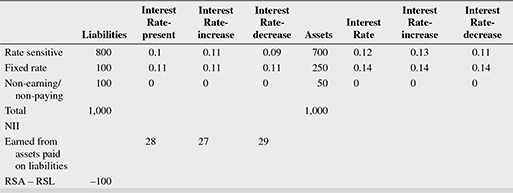
The following inferences can be drawn from Illustration 12.1:
- When GAP is positive, it indicates that the bank has more RSAs than RSLs across the time interval. Such a bank is termed as ‘asset sensitive’
- When GAP is positive, and interest rates rise by equal amounts at the same time for both assets and liabilities, NII increases. The bank would then be paying higher rates on all repriceable liabilities over the time horizon, and earning higher yields on repriceable assets. However, since more assets are repriced than liabilities, NII increases.
- When GAP is positive, and interest rates decrease by equal amounts at the same time for both assets and liabilities, NII decreases for the reason discussed above.
- When GAP is negative, it indicates that the bank has more RSLs than RSAs across the time interval. Such a bank is termed ‘liability sensitive’.
- When GAP is negative, and interest rates rise by equal amounts at the same time for both assets and liabilities, NII decreases. Though both interest income and interest expenses increase, the latter rise more because more liabilities are repriced.
- When GAP is negative, and interest rates fall by equal amounts at the same time for both assets and liabilities, NII increases for the reason discussed in (5).
- Therefore, the sign of a bank’s GAP would indicate whether interest income or interest expenses are likely to change more when interest rates change.
- It also follows that the bank can have a ‘zero GAP’ when RSAs equal RSLs. In this case, equal interest rate changes do not alter NII since changes in interest income equal changes in interest expenses.
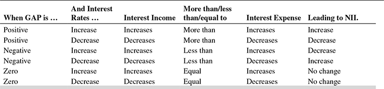
These findings can be generalized in the Table 12.2.
TABLE 12.2 CHANGES IN GAP—SUMMARY OF RESULTS
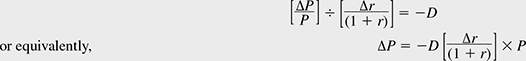
The following simple formula summarizes the framework:
Where ∆NII [expected] represents change in NII from an existing base over a specified period of time,
GAP represents cumulative GAP over the chosen time interval, and
∆r[expected] represents expected changes in the interest rates over the time period
The sign and magnitude of the gaps in various time buckets can be used to assess potential earnings volatility arising from changes in interest rates. A positive gap indicates that RSA are more than RSL and from an earnings perspective, the position benefits from a rise in interest rates. A negative gap on the other hand indicates that RSL are more than RSA and from an earnings perspective the position would benefit from a fall in interest rates. The size of the GAP indicates how much interest rate risk a bank assumes. The utility of this simple approach is that banks can take positions to improve NII for a given level of GAP and forecast of rise or fall in interest rates.
Strengths and weaknesses of this approach: Static Gap analysis is one of the most commonly used approaches to assessing interest rate risk exposure. The principal advantage of this approach is that it is easy to understand and compute. Specific balance sheet items responsible for the risk can be clearly identified, and, once cash flow characteristics of each instrument are determined, GAP measures can be easily calculated.
However, the approach has a number of shortcomings.
First, the analysis makes the simplifying assumption that all positions within a time band mature or reprice simultaneously, thus leading to aggregation that might impact precision of the estimates.
Second, the analysis ignores ‘basis risk’, which arises when loans and other instruments are tied to different base rates or indexes. It is not easy to forecast the frequency or magnitude of changes in market-driven base rates or indexes. This could lead to serious measurement errors.
Third, the analysis ignores the time value of money. The maturity buckets do not clarify whether cash flows arise at the beginning of the period or at the end. For example, if investment in a 1-month treasury bill is financed by an overnight borrowing in the money market, the 1-month GAP is zero, and suggests no interest rate risk. However, when overnight rates rise, the transaction exposes the bank to losses. Therefore, a bank’s gains or losses could also arise from the timing of the repricing or the interest flows within each time interval. Thus even with a zero GAP, the bank’s NII may fluctuate.
Fourth, the short-term focus of GAP measures ignores the long-term impact on fixed rate assets and liabilities. Interest rate changes could have long-term effects on the total risk of the bank’s assets and liabilities.
Fifth, the rate sensitivity of liabilities that bear no interest is ignored. Many banks consider non-interest bearing demand deposits as non-rate sensitive. When interest rates fluctuate, customers’ willingness to maintain demand deposits with banks also changes. It is thus difficult to estimate the exact rate sensitivity of such instruments.
Sixth, the analysis fails to account for differences in the sensitivity of income arising from options embedded in the securities and deposits that banks deal with. Depositors have the option of withdrawing their money before maturity. Similarly, long-term borrowers have the option of prepaying and foreclosing their loans. Such options have different probabilities of being exercised at different interest rate levels. If they are exercised, they can alter the GAP and, hence, the NII as well.
Finally, most GAP analyzes fail to capture variability in non-interest revenue and expenses due to interest rate fluctuations. Volatility in non-interest revenue and expenses is a potentially important source of risk to current net income of the bank.
Hence, GAP analysis, though prevalently used, would provide only a rough approximation of the actual change in NII resulting from the forecasted pattern of change in interest rates. The sign of the GAP does not impact the volatility of NII. It merely indicates whether NII rises or falls when interest rates are expected to fluctuate.
Measuring interest rate risk—Linking the GAP and net interest margin. Some ALM measures focus on the ‘GAP ratio’ while evaluating interest rate risk. The GAP ratio is defined as the ratio of RSAs to RSLs. Thus
When the GAP is positive, the GAP ratio is greater than unity. When the GAP is negative, the GAP ratio will be less than unity.
However, the deficiency in this measure is that does not reflect the size of the interest rate risk a bank assumes. Illustration 12.2 depicts this feature.
ILLUSTRATION 12.2
| Bank A (₹ in crore) | Bank B (₹ in crore) | |
|---|---|---|
| Total assets | 1,000 | 1,000 |
| RSAs | 40 | 400 |
| RSLs | 20 | 200 |
| GAP (RSAs – RSLs) | 20 | 200 |
| GAP ratio (RSAs/RSLs) | 2 | 2 |
| NII (assumed) | 200 | 400 |
| Decrease in interest rate | 2% | 2% |
| Change in NII (GAP × ∆r) | –0.4 | –4 |
In the above example, though the asset size and the GAP ratio are identical for both banks; it is evident that Bank B assumes greater risk since its interest income will be more volatile when interest rates change.
Since interest rate risk is more associated with the volatility in NII, a better risk measure would be one that relates the absolute value of a bank’s GAP to its assets—particularly the earning assets. This ratio can be directly linked to the NIM10 of the bank (see Box 12.3)—the greater this ratio, the greater would be the interest rate risk. The practical implications are that:
- the bank management can determine a target NIM based on the specific risk characteristics of its assets.
- it can determine an allowable variation in the NIM without affecting stakeholder interests.
- based on the above, an acceptable GAP is arrived at.
BOX 12.3 RELATIONSHIP BETWEEN TARGET GAP, EARNING ASSETS AND NIM
The relationship can be evolved as follows:
Hence, NII = NIM × earning assets
The bank determines the acceptable variation in NIM as ∆c. Then, the acceptable variation in NII would be
Since ∆ NII = GAP × ∆r,

Effectively therefore, the relationship between Target GAP and Earning assets can be expressed as a ratio of the product of the expected NIM and the % variability in NIM that can be tolerated, to the expected change in interest rates.
For example, if a bank with earning assets of ₹100 crores expects NIM of 2.5 per cent, but can tolerate variability in the NIM to the extent of ±10 per cent during a year, NIM should fall between 2.25 per cent and 2.75 per cent. If, further, interest rates are forecasted to vary up to 2 per cent during the year, the bank’s ratio of 1-year cumulative target GAP to its earning assets should not exceed 12.5 per cent, as given by the final equation in Box 12.3.
Hence, the bank’s decision to allow only a 10 per cent variation in NIM limits the variation in GAP from –₹12.5 crores to +₹12.5 crores, based on ₹100 crores of earning assets.
It is important to note here the close relationship between a bank’s GAP and its NIM. Hence, in practice, banks limit the size of GAP as a fraction of earning assets, thus, limiting the variation in the NII.
Method 2: Measuring Interest Rate Risk—Earnings Sensitivity Analysis Earnings Sensitivity analysis is an extension of the static GAP analysis. It essentially assesses the impact on net income using ‘what if’ models, carrying out iterations of static GAP analysis assuming different interest rate forecasts and potential interest rate environments. The broad steps of the analysis are as follows:
Step 1 Forecast interest rates assuming various potential interest rate environments
Step 2 Assess the likely changes in the bank’s assets and liabilities by volume and composition under each of these likely environments. The assessment will also examine which of the potential interest rate environments would lead to exercise of embedded options such as loan prepayments or premature deposit withdrawals
Step 3 Assess the likelihood that assets and liabilities would reprice under each of the identified environments. Similarly, identify the implications on off-balance sheet items
Step 4 Calculate the NII under each of the environments, and compare with the ‘base case’ and other scenarios.
The above framework thus helps evaluate the impact of different interest rate environments on the NII, and allows the bank management to set limits for variability of NII or NIM. This approach is sometimes termed as Earning-at-Risk (EAR).
Method 3: Measuring Interest Rate Risk—Rate-Adjusted GAP This method is a simpler variation of the Earnings Sensitivity analysis method described above, and is typically used under circumstances where the complexity and size of a bank’s assets and liabilities and off-balance sheet items are not likely to change dramatically in the short run. The advantage of this approach is that, though simpler, it recognizes the existence of embedded options and different repricing timings. This method is also called ‘Income Statement GAP’ since it uses the balance sheet data to assess the differential impact of interest rate change on each asset and liability class of the bank.
The steps to adopting this approach are as follows:
Step 1 Assess the balance sheet GAP for all items in the balance sheet. This is done by including all balances whose rates are likely to change in, say, the next 12 months
Step 2 Compute the relevant ‘Earnings volatility factor’ (EVF) for each of the balance sheet items. The EVF would reflect the change in the rate applicable to a rate sensitive asset or liability for every 100 bps change in the base rate.
Step 3 The product of the balance sheet GAP and the EVF will reflect the ‘Income statement GAP’, which is the effective GAP estimate, were the interest rates to change as forecasted.
Step 4 Arrive at the impact on NII using the earlier formula
Similarly, the effect on NIM can also be determined using the formula given earlier.
The important advantage of this approach is that it recognizes the value of options and repricing timing in bank assets and liabilities, while being simple to compute. However, the results will depend on the skill of the forecaster to accurately judge the impact of interest rate changes on each class of assets and liabilities.
Illustration 12.3 depicts a simplified usage of this approach. In the example given in Illustration 12.1, we impose differing EVFs on the rate sensitive assets and liabilities.
ILLUSTRATION 12.3

It is evident that assuming different responses to interest rate changes by different assets and liabilities of the bank lead to conclusions quite at variance with the conclusions reached in Illustration 12.1. The rate sensitive GAP is negative and the change in NII is in the opposite direction.
It is, therefore, important that assumptions regarding interest rate movements and their impact on changes in rate sensitive liabilities and assets are done with care and precision in order that misleading conclusions are avoided.
Box 12.4 explores if yield curves do matter for banks’ profitability.
Method 4: Measuring Long-Term Interest Rate Risk—Duration GAP Analysis A fundamental criticism of the static GAP and Earnings Sensitivity analyzes pertain to their preoccupation with short-term interest rate risk in banks. A bank’s assets and liabilities, however, may be mismatched beyond 1 or 2 years and thus expose the bank to substantial risk in the medium or long term. Such risks may go undetected by the traditional GAP approaches.
Hence, banks will also have to look at alternate methods of measuring interest rate risk over the entire life of the assets and liabilities. Duration gap (DGAP) analysis is one such method. As the name suggests, it incorporates estimates of ‘duration’ of assets and liabilities that reflect the value of promised cash flows up to maturity. Hence, it is considered a more comprehensive interest rate risk measure.
Stated in its simplest form, ‘duration’ is the average life of an asset or liability, and is measured as the weighted average time to maturity using present value of the cash flows, relative to the total present value of the asset or liability as weights.
‘Duration’ measures the sensitivity of any instrument to a small change in any of the underlying risk factors. Simply, it is an elasticity measure, providing information on how much a security’s price will change with changes in market interest rates. Annexure II provides the basic concepts, applications and measurement approaches for ‘duration’ and ‘convexity’.
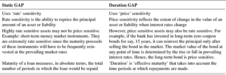
The reasons for using both static GAP and DGAP analyzes in estimating interest rate risk are outlined in Table 12.3.
BOX 12.4 DO YIELD CURVES MATTER FOR BANKS’ PROFITABILITY?
According to theory, it appears logical that the NIM of banks—the difference between interest received and paid as a percentage of earning assets—should be impacted by the slope of the yield curve, i.e., the spread between short- and long-term interest rates. Hence, a flattening yield curve would have an important macroeconomic impact—it may lead to slowing economic growth and consequent pressure on bank earnings. This relationship was seen to be true up to the 1990s. Figure 12.2 shows the trend in relationship in the case of banks in India.
FIGURE 12.2 TRENDS IN RELATIONSHIP BETWEEN YIELD SPREAD AND NIM IN INDIAN BANKS
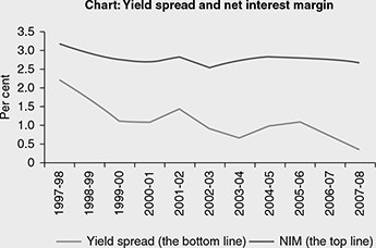
Interestingly, in the recent past, banks’ NIMs appear to show lower sensitivity to yield curve movements. The RBI report on currency and finance (2006–08) attributes the following reasons to this new trend:(a) banks’ diversification into nontraditional activities, (b) banks’ increasing use of derivatives to hedge interest rate risk and(c) banks’ increasing use of noninterest bearing liabilities such as equity and demand deposits to fund assets, when interest yields on assets are declining.
In the case of India, the RBI report notes that there has been a flattening yield curve over the last decade (up to 2006–07). The reason attributed to this is the decline in long-term rates and relative stability of short-term rates. The report also points out that the NIM follows yield spreads with a lag, possibly because lending and borrowing rates of banks are not adjusted instantly to market rate movements.
TABLE 12.3 COMPARISON OF BASIC FEATURES OF STATIC GAP AND DURATION GAP
TEASE THE CONCEPT
As ‘maturity’ of a loan increases, what happens to its ‘duration’?
DGAP analysis examines how interest rate changes would affect the market value of shareholder equity. Similar to the static GAP analysis, the duration of assets and liabilities of a bank are compared over different interest rate environments. After evaluating the impact of interest rate change on the market value of shareholder equity, the DGAP analysis also throws up options for bank management to immunize or insulate market value of equity (MVE) from rate changes.
The steps involved in DGAP analysis are as follows:
Step 1 Forecast interest rate changes for the planning horizon
Step 2 Estimate current market value of the bank’s assets, liabilities and shareholders’ equity
Step 3 Estimate the weighted average duration of assets and the weighted average duration of liabilities, also incorporating the effects of off-balance sheet items, based on the estimated market values.
Step 4 Calculate DGAP
Step 5 Forecast changes in the bank’s MVE under various interest rate environments.
Step 6 Formulate strategies to insulate MVE from interest rate volatility
Box 12.5 derives the relationship between DGAP and the market value of assets and liabilities of a bank.
BOX 12.5 DERIVING THE RELATIONSHIP BETWEEN MVA, MVL AND MVE
The weighted average duration of a bank’s assets is calculated as
and the variables are defined as follows:
wai = the market value of each asset ‘ai’ of the bank divided by the market value of all bank assets (MVA = a1 + a2 + … + an)
Dai = Macaulay’s duration11 of the ith asset
n = number of different bank assets
The weighted average duration of bank liabilities (Dl) is calculated as follows:
And the variables are defined as follows:
wlj = the market value of each liability ‘lj’ of the bank divided by the market value of all bank liabilities (MVL = l1 + l2 + … + lm)
Dlj = Macaulay’s duration of liability j and
m = number of different bank liabilities
We know that Duration is a measure of interest rate sensitivity or elasticity of a liability or asset, which can be represented as follows:
From the above basic equation, we can represent ![]() representing the interest rate.
representing the interest rate.
Since the focus is on insulating MVE from interest rate risk, let us define MVE as the difference between market value of assets and the market value of liabilities, i.e.,
implying that changes in MVE would result from changes in the market values of assets and liabilities.
In the same manner used to determine the change in price given above, we can find the change in the MVE using duration
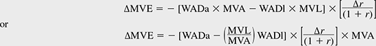
The expression ![]() is the DGAP, and hence
is the DGAP, and hence
The important point to be noted from the expression denoting MVE are as follows:
- The weighted average duration of both assets and liabilities reflect the present value of all promised cash flows in future. Therefore, the need for classifying assets and liabilities into time buckets does not arise.
- The DGAP is ‘leverage adjusted’. Note that DGAP is the difference between weighted average duration of assets and a ‘leverage-adjusted’ weighted average duration of liabilities. This implies that DGAP serves as a rough estimate of the sensitivity of MVE to interest rate changes. The leverage adjustment also denotes how much equity is present to finance the assets and cushion unexpected losses. The interest rate r typically represents an average yield on earning assets. The interest rate assumed here would be an ‘economic interest’ that generates ‘economic income’ as contrasted with ‘accounting income’. ‘Economic Interest’ is simply the product of the market value of each asset and liability and its market interest rate.
- The greater the DGAP, the greater would be the size of the ‘interest rate shock’—the potential volatility in the MVE for a given change in interest rates. Therefore, DGAP serves as a measure of the interest rate risk assumed by the bank, as well as gains and losses to the bank arising from interest rate movements. For example, when DGAP is positive, an increase in interest rates would lower the MVE, while a decrease in interest rates would have an opposite effect and increase the MVE. And when DGAP is negative, an increase in interest rates would increase the MVE while a decrease in interest rates would lower the MVE. These results are in sharp contrast to those from similar static GAP analysis. It also follows that the closer the DGAP is to zero, the smaller the potential change in MVE.
Continuing with the example given in Illustrations 12.1 to 12.3, let us see how duration analysis can be applied to the data. This is demonstrated in Illustration 12.4.
ILLUSTRATION 12.4
Base case: Assumptions:
- All values of assets and liabilities are market values
- Principal is repaid on maturity
- Interest paid yearly
- No defaults, prepayments or early withdrawals
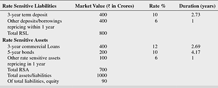
Workings
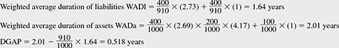
Expected NII = 400 × 12 + 200 × 0.10 + 100 × 0.06 = 400 × 10 = 400 × 0.06 = 10
Sample duration calculations using the basic concept of duration
where, D = duration
t = number of periods in the future
Ct = cash flow to be delivered in t periods
n = term-to-maturity and r = yield to maturity (per period basis).
Sample duration calculations for the above example:

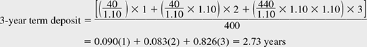
Case 1 Interest rates on both assets and liabilities rise uniformly by 100 bps

| MVA[new] | 18.13 | negative |
| MVL [new] | 13.70 | negative |
| MVE = MVA ‒ MVL | 4.43 | negative |
Thus, the positive DGAP has led to a fall in MVE when interest rates rise uniformly.
The NII is also seen to fall to ₹7.2 crores from ₹10 crores. [This is calculated using market values of assets and liabilities individually from the relationship:
Case 2 Interest rates on both assets and liabilities fall uniformly by 100 bps

| MVA[new] | 18.13 | positive |
| MVL [new] | 13.70 | positive |
| MVE = MVA ‒ MVL | 4.43 | positive |
The NII now increases to ₹12.8 crores from ₹10 crores.
Inferences from Illustration 12.4 are as follows:
- Interest rate risk is evidenced by the mismatch between duration of assets and liabilities, as well as the DGAP of 0.518 years in the base case.
- When there is a change in interest rates, the market values of assets and liabilities would change by different amounts. This would impact the NII in the short term as well as the MVE.
- In the above example, the weighted average duration of assets exceeds the leverage-adjusted weighted average duration of liabilities. This implies that the change in market value of assets will be greater than the market value of liabilities, if all rates change uniformly. Case 2 demonstrates that with a uniform increase of 100 bps in interest rates, market value of assets declines by a greater margin (₹18 crores) than market value of liabilities (₹14 crores). MVE is estimated to fall by ₹4 crores.
- In case 2, there is also a decrease in the expected NII when the interest rate increases. The explanation is simple—the bank will have to pay more for refinancing its assets when the liabilities mature (since the duration of liabilities is less than that of assets).
- Further, the following table shows that there is an increase in the bank’s overall risk with an increase in interest rates due to changes in the market values of assets, liabilities and consequently, equity.
(₹ in crores) New (case 1 – interest rates increase) Existing (base case) MVA 983 1000 MVL 896 910 MVE 87 90 MVE/MVA 0.088 0.09 MVA/MVE 11.30 11.11 MVE/MVA is an approximate indicator of the bank’s capital adequacy,12 while the inverse of this indicator is the equivalent of the equity multiplier (EM).13 The former shows a decline, and the latter an increase over the base case, in the wake of an interest rate increase—both pointers to increased risk for the bank.
- Case 2, reflecting the impact of decrease in interest rates, shows opposite results. The duration mismatch leads to greater increase in market value of assets than market value of liabilities and, therefore, an increase in the MVE. NII also improves, and so do other indicators such as MVE/MVA and the EM, and it appears the bank is better off.
The above inferences are generalized in Table 12.4 as follows:
TABLE 12.4 CHANGES IN DGAP—SUMMARY OF RESULTS
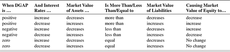
Also note that the impact on NII is contrary to the results seen in the case of static maturity GAP.
How can duration be used as a tool to assess and manage interest rate risk? Though a static measure, DGAP can be employed in assessing the changes in MVE during periods of volatile interest rates. The greater the absolute value of the DGAP, the more is the interest rate risk. However, a bank would ideally desire to sustain the MVE or maintain an increasing trend, given the volatility of interest rates.
‘Immunizing’ Market Value of Equity From Table 12.4, a bank will have to operate with its DGAP at zero, if it desires to maintain its MVE while interest rates change. This implies that the bank’s average asset duration should be slightly below the average liability duration. More specifically, the average asset duration for a bank with DGAP at zero should be equal to the product of the bank’s liability duration and a factor that represents the ‘leverage’ (MVL/MVA).
To set DGAP to zero, three alternative courses of action can be followed:
- Adjust the duration of market value of assets
- Adjust the duration of market value of liabilities
- Adjust the market values of both assets and liabilities
In practice, it is easier to adjust the duration of the market value of assets. To do this, we would have to set DGAP = 0 in the equation WADa – (MVL/MVA)WADl = DGAP. That is,
In Illustration 12.4, where the DGAP 0.518 arises from the difference between 2.01 (WADa) and 1.49 (WADl × MVL/MVA), DGAP can be made zero if: (a) the weighted average duration of assets is reduced to 1.49 years, or (b) the weighted average duration of liabilities is increased to 2.21 (2.01/0.91) years, or (c) use some combination of these adjustments.
Under (c), a deliberate mismatch is maintained to enable immunize the MVE. This is done by segregating the term WADa – WADl from the DGAP equation after setting DGAP = 0, as follows:
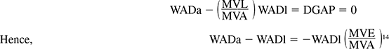
That is, from Illustration 12.4,

This implies that the bank in Illustration 12.4 can maintain the MVE if it can carry a duration mismatch, such that
Other Target Variables Used for Immunizing Interest Rate Risk
Net interest income (NII) and market value of equity (MVE): Banks are sometimes interested in immunizing the market value of equity and NII simultaneously or independently. In such cases, variations of the immunization process are used. For instance, Toevs (1983)15 sugggests that a bank can alternatively hedge or immunize its NII and MVE, as given below.
Since MVE = MVE – MVL, MVA × duration of assets (DA) should equal MVL × duration of liabilities (DL ) if MVE is to be immunized.
It follows that if MVE should be positive, then DL should exceed DA.
DA = (MVANS × DNSA + MVARS × DRSA )/MVA and DL = (MVLNS × DNSL + MVLRS × DRSL )/MVL, where NS, RS signify Non rate sensitive and Rate sensitive, respectively to immuise MVE.
Therefore, setting MVA × DA = MVL × DL to immunize MVE, the equation can be rewritten as MVA × (MVANS + DNSA + MVARS × DRSA)/MVA = MVL × (MVLNS × DNSL + MVLRS × DRSL )/MVL
or
MVANS × DNSA + MVARS × DRSA = MVLNS × DNSL + MVLRS × DRSL
Adding and subtracting MVE and MVL on the respective sides of the equation,
MVANS (DNSA – 1) + MVA – MVARS (1 – DRSA ) = MVLNS (DNSL – 1) + MVLRS – MVLRSL (1 – DRSL )
or
MVANS (DNSA – 1) + MVE = MVLNS (DNSL – 1) + DGAP
According to Toevs, if a bank wishes to hedge NII and immunise MVE, DGAP should be set to Zero, and MVANS (DNSA – 1) + MVA equal to MVLNS (DNSL – 1) + MVL.
Alternatively, if the bank wishes to immunize MVE even at the cost of NII, it can select a non zero DGAP, while keeping the above eqality intact.
A bank can put its MVE at risk and hedge its NII by setting DGAP = 0 but not fulfilling the above equality.
Dynamic duration GAP analysis: As done in the static GAP earnings sensitivity analysis framework described above, a sensitivity analysis for MVE also called Economic Value of Equity (EVE) can be carried out through simulation models. The sensitivity analysis assesses the impact of various interest rate environments on MVE through ‘what if’ analysis. The volatility in the MVE compared with the base case or the most likely scenario would be the indicator of interest rate risk. Some of these models are also capable of assessing the impact of customers exercising embedded options, or shifts in the yield curve, or varying yield spreads.
TEASE THE CONCEPT
What is the expected impact on ‘duration’ if the following options were exercised?
- A large deposit is withdrawn before maturity
- A large loan is repaid before maturity
Strengths and weaknesses of the ‘duration’ approach: The primary strength of ‘duration analysis’ lies in its ability to provide a comprehensive measure of interest rate risk for the entire portfolio of the bank—assets, liabilities and surplus (equity). The smaller the absolute value of DGAP, the less sensitive the MVE is to interest rate changes.
The approach is considered more practical than the static GAP approach, since cash flows over the entire life of each asset and liability is taken into account while computing duration. Thus, the time value of each cash flow is recognized. Further, this feature obviates the need for classification of assets and liabilities into different time buckets.
Duration analysis enables the bank to match assets and liabilities at an aggregate level and assess the impact of interest rate risk, a feature that is not possible in static GAP analysis.
The long-term, aggregate view that duration analysis offers is valuable, since bank management acquires flexibility to adjust rate sensitivity using a variety of hedging instruments.
However, ‘duration analysis’ is not without limitations.
- First, duration measurement calls for several subjective assumptions, and, hence, the ‘duration’ may not be computed accurately.
- Duration is based on ‘promised’ rather than ‘expected’ cash flows. Exercise of embedded options, or change in default probabilities could render initial forecasts invalid. Hence, a bank should have systems in place to monitor whether actual cash flows conform to initial cash flow forecasts.
- Even while using sophisticated simulation models for sensitivity analysis, the need for forecasting customer behaviour on when embedded options would be exercised, or the value of these options, build in subjectivity and complexity into the model.
- Duration analysis requires that each cash flow be discounted by an appropriate discount rate, to arrive at the present value of future cash flows. Identifying appropriate discount rates for various cash flow streams, therefore, becomes a crucial but complex step in arriving at the likely impact of interest rate risk.
- We have seen that immunizing market value sensitivity requires continuous monitoring and adjustment of the portfolio’s duration. Such adjustments could also mean potential restructuring of a bank’s balance sheet, which may not be practically feasible.
- Theoretically, duration calculations have been found valid only for small changes in interest rates. In other words, with larger interest rate increases, duration over-predicts the fall in bond prices, while for larger interest rate decreases, it under-predicts the rise in bond prices. This is because the bond–price relationship is convex, and not linear, as assumed by the duration model.
- Duration of the market value of assets and liabilities are likely to keep changing over time and require continuous monitoring and balancing.
- Finally, it is a challenge to estimate the duration of assets and liabilities that do not earn or pay interest. For example, how will interest rate changes impact the level of non-interest bearing demand deposits maintained by borrowers? In the absence of fixed or promised cash flows in this important segment of bank liabilities, any assumptions made about cash flows could turn out to be inaccurate. However, fluctuations in these deposits have the potential to impact the DGAP and MVE sensitivity.
It can therefore be concluded that: (a) larger convexity of a security signifies larger interest rate protection, (b) the more the convexity, the larger the error of using just duration to immunize against interest rate changes, and (c) all fixed income securities are convex.16
Hence, bank management would prefer to capture the effect of such convexity in their interest rate risk management models
Managing Interest Rate Risk—A Strategic Approach
Let us begin with the understanding that financial risk and interest rate risk are an integral part of banking business. However, if these risks are not managed, the bank’s profitability and solvency are at stake. The issues in managing interest rate risk, therefore, are to determine how much risk is acceptable to the bank, and the strategies to achieve and maintain a desired optimum risk profile.
We have seen that it is theoretically possible to manage interest rate risk by strategically varying static GAP or DGAP. How difficult is it to actually implement these approaches? For instance, can interest rates be forecasted accurately into the future? Even if such forecasting is possible, can the variations in GAP or DGAP be without other implications, such as the impact on the bank’s profitability? How much control do banks have over a customer’s selection of deposit or loan products?
Let us look at some of the strategies banks could follow to achieve the desirable GAP position. To reduce asset sensitivity, banks have the following alternatives. They could (a) extend the maturities in the investment portfolio, (b) increase floating rate deposits, (c) increase short-term borrowings, (d) increase long-term lending, (e) increase fixed rate lending and so on. Similarly, to reduce liability sensitivity, banks could do the opposite—such as, reducing the maturity of the investment portfolio, or increasing long-term deposits, or increasing shortterm lending or increasing floating rate lending, and so on.
Hence, the basic balance sheet strategy to manage interest rate risk is to effect changes in portfolio composition. However, it has to be borne in mind that any variation in portfolio has a potential impact on NII. Illustration 12.5 describes the possible impact of two specific strategies adopted by a bank.
ILLUSTRATION 12.5
- Bank A has a negative GAP over the time horizon of the next 1 year. This implies that the bank has a positive DGAP.
- Bank A expects interest rates to rise
What should Bank A’s strategy be for managing interest rate risk?
According to our earlier discussion, the bank would take measures to drive the GAP towards zero. Or, if the objective were a stable MVE, the bank would fine-tune its DGAP to shorten the average asset duration and lengthen the average liability duration.
Let us examine some of these strategies, say, where the bank shortens the maturity of its investment portfolio, and increases the rate on long-term deposits to attract more long-term depositors.
However, in implementing these strategies, the bank has explicitly decided to (a) sacrifice some yield from short-term investment, and (b) increase its interest costs in the short term. Both tend to reduce the bank’s NII and NIM for the year. Then why is the bank embarking on this strategy? Since it expects to gain from stalling a potential NII or MVE fall when interest rates rise.
However, the bank has made a critical assumption here. Only if the interest rates rise above the current assumed forward rates,17 will the bank’s investment in short-term securities (versus long-term securities), or its preference for longterm deposits (over short-term deposits) translate into a gain for the bank. If the rates remain below the assumed forward rates, short-term securities would yield much less than long-term investments, and the bank would end up paying more on its long-term deposits as well.
The inference from Illustration 12.5 is obvious. Bank A’s management is adjusting GAP and DGAP, and basing such adjustments on its interest rate forecast, which could turn out to be accurate or inaccurate.
Interest Rate Risk or Model Risk?
Most banks prefer to develop and run their own models for interest rate risk measurement. Because different models tend to use much of the same information, but the results may be different, banks have to decide which model and results to use for its purposes.
A bank can get radically different results from the models by merely changing the assumptions on which the model is built. Therefore, it is important to be aware of the assumptions that were used to generate the results and the bank has to make some judgment about their plausibility. For instance:
- What interest rate assumptions have been made and what maturity assumptions have been used for deposit accounts without specified maturities?
- What assumptions were made with respect to the optionality in the bank’s assets and liabilities? What business strategies were incorporated into the analysis?
- What assumptions were made regarding customer behaviour as interest rates change?
- Have assumptions changed since the last time the model was used? If so, why?
The best way to assess the reliability of the output of models is to ask questions about the assumptions to see if they seem realistic and cover all possibilities. Also, special attention should be paid to the worst-case scenarios, since worst-case situations often result in serious problems for banks in the unlikely event of their occurrence. Bank Management should always be thinking about new ways to hedge against these extreme situations.
Alternative Methods to Reduce Interest Rate Risk
According to Hingston (2002),18 there are four basic methods to mitigate interest rate risk in financial institutions—(a) selling assets, (b) extending liabilities, (c) off-balance sheet hedging and (d) retaining status quo. While evaluating these alternatives, Hingston has concluded as follows:
- Selling fixed rate, long-term assets may reduce interest rate risk exposure, but could also lead to losses on such sale that may undermine the selling bank’s capital
- By obtaining matching fixed rate, long-term liabilities to fund fixed rate and long-term assets, a bank may theoretically be able to reduce interest rate risk. However, this could create losses in a declining interest rate scenario;
- If the Board so decides, a bank may decide not to do anything about reducing interest rate risk.
This brings us to the final alternative strategy for managing interest rate risk—interest rate derivatives.
SECTION IV
MANAGING INTEREST RATE RISK WITH INTEREST RATE DERIVATIVES
Bank A in Illustration 12.5 can explore yet another alternative to mitigate the interest rate risk on its investments—it can use interest rate derivatives (IRDs) to transform some of its fixed rate investments into floating rate assets. It can also use IRDs to transform floating rate liabilities into fixed rate liabilities.
What do IRDs do? Simply, they are contracts that are used to hedge other positions that expose them to risk, or speculate on anticipated price moves. In most cases, banks use IRDs to replicate balance sheet transactions with off-balance sheet contracts, so that contingent positions are created.
Interest Rate Derivatives, as their name suggests, are financial instruments whose value depends on the value of other underlying instruments (such as the price of underlying fixed rate securities) or indices (such as interest rate indices). They have a variety of advantages over other interest risk mitigating approaches:
- They allow banks to completely customize their interest rate risk profile.
- Since the derivatives can replicate the interest rate exposure of fixed income securities without the requirement of an upfront investment, they may have lower credit risk and greater liquidity.
- Sometimes, use of IRDs could lower transaction costs.
- The accounting and regulatory treatment of IRDs are getting to be fairly streamlined.
The IRDs function as tools that banks can use to ‘actively’ manage interest rate risk. There are a variety of such tools, and we will be discussing the most important and prevalent among these in the ensuing paragraphs. Given that bank management would prefer to manage, rather than totally eliminate interest rate risk, these tools can be used to complement existing strategies (as discussed in earlier sections) aimed at immunizing the volatility of earnings and MVE to changes in interest rates.
In this chapter, we will focus on the most basic and widely used contracts—swap contracts, financial futures, forward rate agreements (FRAs), options, caps/floors/collars and ‘swaptions’ (swap options).
Swaps
A swap is an agreement in which two parties (counterparties) agree to exchange periodic payments. The monetary value of the payments exchanged is based on a notional19. principal amount. Swaps are classified based on the characteristics of swap payments. There are four prevalent types of swaps—currency swaps, interest rate swaps, commodity swaps and equity swaps.
Traditionally, banks managed interest rate risk by adjusting the maturity or repricing schedules of their assets and liabilities. As described earlier in this chapter, a bank wishing to lengthen the duration of its assets can add long-term securities to its investment portfolio.
However, banks have now found that the same goal can be accomplished more efficiently and cost-effectively by entering into plain ‘vanilla’ swaps—where they pay a floating rate, usually based on the London Inter bank Offered Rate (LIBOR) or a market-determined prime rate of the country (where such a rate exists), and receive a fixed rate, which could typically be the treasury rate of equivalent maturity plus a premium. A liability sensitive bank, on the other hand, can enter into a swap where it pays a fixed rate and receives a floating rate. Banks can also use ‘basis swaps’ where both sides pay floating rates but the index rates are linked to the banks’ cost of funds and yield on advances. In such cases, specifically, the banks would pay the prime lending rate and receive LIBOR.
In a ‘pure’ interest rate swap, one party X agrees to pay the other party Y, cash flows equivalent to a predetermined floating rate interest on a notional principal for a specified number of years. Simultaneously, Y agrees to pay X cash flows equal to fixed rate interest on the same notional principal for the same period of time. The currencies of the two sets of cash flows are also the same.
Interest rate swaps were basically developed to satisfy borrowers’ need for fixed rate funds. Banks typically hesitate to fund less creditworthy borrowers on a fixed rate basis (simply because banks do not fund themselves on a fixed rate basis), but may be willing to lend at floating rates.
Illustration 12.6 would help to understand the concept better.
ILLUSTRATION 12.6 HOW DO INTEREST RATE SWAPS WORK?
Firm A, with credit rating less than investment grade, requires ₹100 crore fixed rate funding for a term of 7 years. The firm has two alternatives—(a) borrow 7-year, fixed rate funds at a sizeable premium, say, at 12 percent per annum, or (b) borrow floating rate funds for the 7-year period at a small premium, say at the market-determined prime rate (equivalent to LIBOR) plus 2 percent per annum
Firm B, which enjoys investment grade credit rating, requires floating rate funds. Moreover, it can issue 7-year fixed rate bonds in the same currency, at say, 10 per cent per annum. It can also acquire floating rate funds for an equivalent term at the market determined prime rate (equivalent to the LIBOR) plus 50 bps per annum.
The rates offered to the firms can be represented as follows:
| Fixed Rate | Floating Rate | |
| Firm A | 12% | LIBOR + 2% |
| Firm B | 10% | LIBOR + 0.5% |
The advantage enjoyed by Firm B is termed ‘absolute advantage’, since it is able to negotiate lower rates in both fixed and floating rate markets. It can also be seen that firm A’s cost of funds is higher in the fixed rate market by 2 per cent [12% − 10%] and 1.5 per cent in the floating rate market [LIBOR + (2% − 0.5%)]. This is termed as A’s ‘relative advantage’ in the floating rate market. This advantage is also called ‘comparative advantage’. Thus, from the above argument, A has comparative advantage in the floating rate market. It follows that if A and B borrow in the markets where they enjoy comparative advantage, and then swap the borrowing, the cost of funds for both firms can be reduced.
Now, assume that Firm A wants to borrow funds at a fixed rate, and Firm B prefers to acquire funds at a floating rate linked to the LIBOR. Firm B appears to have comparative advantage in the fixed rate market. The fact that the difference between the two fixed rates is greater than the difference between the two floating rates, allows a profitable swap to be negotiated. This is done as follows:
Firm A would raise floating rate funds at LIBOR + 2%, and Firm B would raise an identical amount of fixed rate funds at 10 per cent. Next, A and B enter into a swap such that A ends up with fixed rate funds and B ends up with floating rate funds.
In most swap transactions in practice, a swap dealer serves as an intermediary. However, to understand the concept better, let us assume that A and B effect the swap directly without an intermediary. They might negotiate the following type of swap:
Firm A agrees to pay B fixed interest at, say, 9.75 per cent, and B agrees to pay A floating interest at LIBOR percent per annum.
How is the swap advantageous to both sides?
Let us consider B, which has three sets of interest rate cash flows: (a) it pays 10 per cent to outside lenders, (b) it receives 9.75 per cent per annum from A and (c) it pays the LIBOR to A. The net effect of cash flows (a) and (b) is a cost of 0.25 per cent per annum to B. The net effect of all three cash flows is that B pays LIBOR + 0.25%, or 0.25% less than what it would have had to pay to the floating rate markets if accessed directly.
Firm A also has three sets of cash flows: (a) it pays LIBOR + 2% to outside lenders, (b) it receives LIBOR from B and (c) it pays 9.75 per cent per annum to B. The first two cash flows aggregate to a cost of 2 per cent, and all three taken together implies that A pays 11.75 per cent per annum for obtaining fixed rate funds, or 0.25 per cent less than if it had gone directly to the fixed rate markets.
Therefore, it is evident that an interest rate swap benefits both A and B by 25 bps each, i.e., an aggregate gain of 50 bps per annum. This figure of 50 bps is nothing but the difference between 2 per cent (the difference between the rates at which A and B could access funds in the fixed rate market) and 1.5 per cent (the difference between the rates at which A and B could access funds in the floating rate market).
Thus, generalizing, the total gain in an interest rate swap can be represented as x − y, where x is the difference between the interest rates facing the counterparties in the fixed rate market, and y the difference between the interest rates facing the counterparties in the floating rate markets.
The advantages to Firm B (inferred from Illustration 12.6) can be summarized as follows:
- It could achieve a lower cost borrowing from the floating rate market
- It could match its assets and liabilities
- It eliminated interest rate and refinancing risks
The advantages to Firm A are summarized as follows:
- It could achieve a lower cost of borrowing from the fixed rate market
- Its capacity to access the fixed rate market in future remains intact
- It saved the cost and time involved in a public issue
- It constituted an off-balance sheet transaction
- The higher cost of borrowing in the fixed rate market would have been accompanied by more stringent covenants, which the firm avoided by opting for the swap
Banks can serve as counterparties or intermediaries in swap transactions.
In Illustration 12.6, the swap involved only two parties. However, in practice, since it is difficult to find two entities with equal and opposite needs, intermediaries facilitate the transaction. Illustration 12.7 would serve to clarify the situation where the intermediary brings together the counterparties in a swap arrangement. In such a case, it is evident that the total benefit from the swap must be shared with the intermediary.
In Illustration 12.6, the total benefit from the swap was 50 bps. If the intermediary’s fee is 10 bps, and the benefit of the swap is being shared equally by the two counterparties, each party will still be able to lower its cost of funds by 20 bps each. Banks can play the role of intermediaries effectively due to their strategic position and experience in the financial markets.
ILLUSTRATION 12.7
In Illustration 12.6, if the intermediary, say Bank X, demands a 10 bps fee, the cash flows would be as follows:
Firm A—(a) pays lenders in floating rate market at LIBOR + 2%, (b) receives LIBOR + 0.3% from Bank X and (c) pays 10.10 per cent to Bank X. The net effect of (a) and (b) is 1.7 per cent. Adding 10.10 per cent from (c) takes the total outflow to A to 11.8 per cent. If A had accessed the fixed rate markets it would have had to pay 12 percent. Thus, A has gained 20 bps from the swap transaction.
Firm B—(a) pays 10 per cent to lenders in the fixed rate market, (b) pays LIBOR + 0.3% to Bank X and (c) receives 10 per cent from Bank X. Its total outflow, therefore, is LIBOR + 0.3%. If it had accessed the floating rate market, B would have had to pay LIBOR + 0.5%. Therefore, B has gained 20 bps from the swap transaction.
Bank X—(a) receives 10.10 per cent from A, (b) receives LIBOR + 0.3% from B, (c) pays LIBOR + 0.3% to A and (d) pays 10 per cent to B. The net effect of the four transactions is a gain of 10 bps for Bank X.
It may be noted that the total gain from the swap remains at 50 bps, the difference between the net interest rates in the fixed rate and floating rate markets.
Illustration 12.8 introduces basic market terminologies in the swap market.
ILLUSTRATION 12.8 USING MARKET TERMINOLOGIES
Let us assume that in the swap market, firm A wants to enter into a swap transaction with Bank X for a period of 2 years. Firm A and Bank X enter into the contract on 1 June 2009. According to the contract, A will pay semi-annually the interest of 10.10 per cent per annum to X, while the bank will pay A semi-annually at the floating rate of LIBOR + 0.3%.
In this connection, the terminologies typically used in the swap market are as follows:
- The ‘trade date’ is the date the parties agree to a swap. In this case, it is 1 June 2009
- ‘Value date’ is the date on which the initial fixed and floating payments begin to accrue—that is, 2 days after the trade date. This is also called the ‘effective date’. If the effective date is after 2 days of the trade date, it is called the ‘spot date’. The maturity of a swap contract is computed from the effective or value date. In the example, if the value date is 3 June 2009, then the effective date, spot date and value date would be the same.
- ‘Maturity date’ is the date on which interest accrual ceases
- ‘Reset date’ is the date on which the applicable LIBOR will be determined for payment of semi-annual interest. In our example, the first payment is due on December 3, 2009, i.e., 6 months from the value date and the second payment on 3 June 2010. The 6-month LIBOR relevant for calculating the second payment will be reset based on the rate prevailing 2 days before the first payment date, i.e., on December 1, 2009. This sequence will be usually followed for the remaining period of the swap contract, unless otherwise specified in the contract.
How are swaps applied in practice to manage banks’ interest rate risk?
- Adjusting the rate sensitivity of an asset or liability: Consider the following example. Bank C has made a loan of ₹100 crore with 5 year maturity to a prime customer at a rate of 10 per cent. The corresponding liability is a 6-month deposit of ₹100 crore, at a floating rate linked to the prevailing market-determined 6-month prime rate. Obviously, there exists an interest rate risk in this transaction. Every time the prime rate rises, the bank makes a loss on the transaction, apart from the bank having to seek refinance for the loan every 6 months (at higher rates, if interest rates are rising). Assume the bank wants to hedge this transaction through a swap, and it agrees to pay, say, 6 per cent, and receive 6-month prime rate against ₹100 crore for 5 years till the loan is fully paid. The net effect on the bank’s balance sheet would be as follows—(a) the bank would earn 10 per cent from the loan + 6 month prime from the swap, and (b) the banks would pay 6 month prime for the rupee deposit + 6% from swap as agreed upon. The net spread on this transaction would therefore be 4 per cent (10% − 6%, the receipt and payment of prime cancelling out). The bank has thus locked in a liability cost of 6 per cent (the bank paying and receiving prime every 6 months). Thus, the use of the swap has helped the bank not only reduce interest rate risk, but also to lock in a spread of 4 per cent on this transaction. In general, a swap can help adjust the rate sensitivity of an asset or liability by converting a fixed-rate loan-floating rate, or a floating-rate liability fixed rate, and so on.
- Creating synthetic transactions and securities: Swaps are considered ‘synthetic’ since they are off the bank’s balance sheet. Are off-balance sheet transactions less risky than balance sheet transactions? Capital adequacy requirements20 mandate holding of capital against off-balance sheet positions, which implies that there are risks21 associated with these positions. Of course, the bank can do away with the need for a swap and match the 5-year asset in the previous example with a long-term deposit with equal or longer tenor, or exit the swap midway. The decision to create a ‘synthetic’ security would, therefore, be dependent on whether the yield advantage of the swap exceeded the costs (and risks) of such transactions.
- Adjusting the GAP or DGAP to immunize earnings or MVE: A liability sensitive bank with a positive DGAP will resort to a swap that would produce profits even when interest rates increase. This can be achieved by adjusting asset duration or increasing RSAs. A swap that pays fixed and receives floating is comparable to increasing RSAs over RSLs. Similarly, a bank with a negative DGAP will want to hedge by taking a swap position that would produce profits when interest rates fall.
Box 12.6 summarizes the key points to be kept in mind in respect of interest rate swaps.
BOX 12.6 INTEREST RATE SWAPS—SUMMARIZING KEY POINTS
- Interest rate swaps are off-balance sheet items.
- A primary objective of the swap is to save on interest cost. Therefore, the prevailing relationship between borrowers and lenders does not change.
- The major swap market players are banks or other intermediaries and corporate entities.
- The swap contract is distinct from the original loan contract. Hence, the swap tenor is independent of the loan maturity.
- Where the differential in fixed rate is greater than the differential in floating rate available to counterparties in a swap, a switch from fixed to floating rate is carried out.
- Where the differential in floating rate is greater than the differential in fixed rate available to counterparties in a swap, a switch from floating to fixed rate is carried out.
- The credit risk in a swap arrangement is restricted to interest payments only, and does not affect the notional principal amount agreed upon by the counterparties.
- Pricing of the interest rate swap involves forecasting future benchmark rates. Some common techniques involve the use of yield curves of government securities, forward interest rates or zero coupon securities.
- Swaps can be used for liability management, and could lead to speculative gains.
Interest Rate Futures
A futures contract is a legal agreement between a buyer (or seller) and an established exchange in which the buyer (or seller) agrees to take (or make) delivery of something at a predetermined price at the end of a predetermined period of time. The price at which the parties agree to transact in the future is the ‘futures’ price. The predetermined date at which the parties must transact is the ‘settlement’ or ‘delivery’ date.
Futures can be categorized as financial or non-financial futures. Commodity futures (which were the only known futures prior to 1972) are non-financial futures. Financial futures are contracts based on a financial instrument or financial index. The most commonly known financial futures are (a) stock index futures, (b) interest rate futures, and (c) currency futures.
When the underlying asset is an interest-bearing security, the contract is termed ‘interest rate futures’. Interest rate futures contracts are typically classified by the maturity of the underlying security. Short-term interest rate future contracts are those whose underlying securities mature in less than 12 months. A long-term futures contract is, therefore, one whose maturity exceeds 1 year.
The major function of the futures markets is to transfer the interest rate risk from the ‘hedger’22 to the ‘speculator’.23
In the futures market, hedging acts as a temporary substitute for a transaction to be made in the cash market, locking in a value for the cash position at some point of time. When cash and futures prices move together, a ‘perfect hedge’24 is possible where the profit in one market is equally offset by a loss in the other. Box 12.7 outlines some basic principles of hedging in the futures (and forward) markets.
BOX 12.7 BASICS OF FUTURES (AND FORWARD) CONTRACTS
Differences between futures and forward contracts
A forward contract, like a futures contract, is an agreement to deliver something at a predetermined price at the end of a predetermined period. Forward contracts differ from futures contracts in the following aspects: (a) futures contracts are standardized agreements in respect of delivery dates and quality of the deliverable, while forward contracts are essentially non-standardized, since the terms of each contract are negotiated individually between buyer and seller, (b) futures contracts are traded on recognized stock exchanges, while forwards are over the counter (OTC) instruments, (c) there is a very thin or non-existent secondary market for forward contracts, (d) forward contracts are intended for delivery, while futures may not be intended to be settled by delivery, (e) futures are marked to market at the end of each trading day, while the marking to market of forward transactions are by mutual agreement between the counter parties, (f) interim cash flows are possible in futures contracts, either as additional margin in case of adverse price movements or as cash withdrawn in case of favourable price movements, while such interim cash flows can occur in forwards not marked to market, and, importantly, and (g) the credit risk due to counter party default inherent in a forward contract is mitigated due to the transaction being guaranteed by the exchanges.
Simple examples of trading in interest rate futures
An interest rate futures contract is an agreement for buying or selling a standard quantity of specific interest-bearing instruments, at a price agreed upon by the parties, at a predetermined date in future.
Firm A has a fixed-rate loan contract with Bank B. It expects interest rates to fall. One alternative is to buy a futures contract. If the current interest rate is 10 per cent and the firm expects the rate to fall to 9 per cent, it can buy a futures contract at market price. If the interest rate does fall, the contract will quote higher (since when interest rates fall, instruments offering higher coupon rates rise in value). The firm sells the futures and gains.
Similarly, if the firm expects interest rates to rise, and it has a floating-rate loan contract, it would sell futures at market price. When interest rates rise, the futures contract will quote lower for the same reason stated above. The firm now buys the futures and gains.
In general, when a firm has an asset portfolio, it could:
- buy interest rate futures if it expects interest rates to fall, and
- sell interest rate futures if it expects interest rates to rise.
Similarly, when a firm has a liability portfolio, it could:
- sell interest rate futures if it expects interest rates to fall, and
- buy interest rate futures if it expects interest rates to rise.
A brief look at how futures trading takes place
Futures contracts are traded on organized exchanges25 that also serve as clearing houses. The likelihood that the counter party to a forward contract defaults in his obligations is eliminated in futures contracts, since the exchange assumes all obligations at the end of each trading day, forcing members to settle their net positions.
In practice, a buyer and seller are found for each transaction, and the procedure enables any trader to offset an initial position by assuming the opposite position any time prior to the futures contract’s delivery date. For example, a buyer of a T-Bill futures contract for, say, 90 days, can offset his position by selling the same contract, say, a fortnight later. The liquidity that this procedure affords is a feature of the futures market, not found in a forward contract. The liquidity is a result of trading standardized assets through the exchange.
Once the futures contract is entered into, there are cash flow obligations for buyers and sellers. While entering into the contract, traders must deposit an ‘initial margin’ with the exchange that serves as a cash margin that would partially offset losses arising from adverse rate movements.
Apart from the initial margin, the exchange also requires traders to meet a ‘maintenance margin’, specifying the minimum deposit required at the end of each trading day. These margins are not to be confused with margins for stocks discussed in earlier chapters on Credit Administration. The futures margin deposits are similar to performance bonds—the trader guarantees that mandatory payment obligations will be met. In case the margin deposit falls below the specified minimum requirement, the trader must deposit more funds.
The maintenance deposit varies with the movements of the underlying asset in the market, and, hence, the exchange identifies the change in the value of every trader’s account at the end of every day, crediting the margin account of the trader with gains and debiting with losses. This daily settlement process is termed ‘marking to market’.
On the date of contract expiration, trading is halted, and the traders settle their final positions. Contracts can be settled either through physical delivery or cash settlement. In the case of physical delivery, the seller of futures delivers the physical asset, while the buyer makes cash payment to the seller. In cash settlement, there is no physical delivery, and traders merely settle the final value of the position after the last trading day.
‘Basis’ risk of hedging
In practice, futures contracts may not work perfectly due to the following possibilities: (a) the hedge may require that the futures contract be closed before its expiration date, (b) the asset whose price is to be hedged may not be identical to the asset underlying the futures contract, or (c) the hedger may be unsure of the exact date when the asset would be bought or sold.
(a) is the result of futures contracts being standardized. An example for (b) would be using rupee futures to hedge price movements of commercial paper transactions. The situation in (c) could arise from the seller’s uncertainty regarding delivery date of a product consequent to certain troubles experienced by the firm producing the product.
Any of the situations outlined above could give rise to ‘basis risk’
‘Basis’ is simply the profit (or loss) on the hedge. It is determined by the difference between the cash price (also called the ‘spot’ price) of the asset to be hedged and the futures price when the hedge is placed, and when the hedge is lifted. Thus,
Theoretically, the basis is also the ‘cost of carry’ or the net cost of financing a position, i.e., the difference between the rate of financing and the cash yield from holding the underlying asset.
If the asset to be hedged and the underlying asset of the futures contract are identical, the basis should be ‘zero’ when the futures contract expires. Before expiration, the basis can be positive or negative.
The above definition of basis shows that when the spot price increases more than the futures price, the basis will also increase or ‘strengthen’. Similarly, when the futures price increases more than the spot price, the basis decreases or ‘weakens’.
Basis risk in hedging arises when the basis changes at the time of removing the hedge. Hence, the actual risk in hedging interest rate movements is not that the level of interest rates will move against the cash position, but that the basis might change between the time the hedge is initiated and removed. The effective return from the hedge can be expressed as the difference between the initial cash rate and the change in basis.
Generally, movements in the basis are more predictable than movements in the spot market rates and the volatility of spot rates are typically more pronounced than the volatility of the basis. This explains why in most cases it is less risky to hedge than not hedge at all. Even where sizeable changes occur in the basis, it is to be noted that the predominant factors that influence the spot markets simultaneously influence futures markets as well. Further, with arbitrage activity, basis could be driven to zero levels as time to expiration approaches, if the cash instrument to be hedged is the same as the asset underlying the futures contract.
Basis risk and cross hedging
In not all cases is the asset to be hedged identical to the asset underlying the futures, as assumed above. In such circumstances, ‘cross hedge’ is used.
Though cross hedging is common in many hedging applications, the risk potential is also greater in cross hedges since futures and spot interest rates based on different underlying assets may not always move together in the same direction. According to the measure of effective return given above, the volatility of the return depends on the volatility of the basis.
In most cases, the effectiveness of a cross hedge is determined by (a) the relationship between the spot price of the underlying asset and its futures price when a hedge is initiated and when it is removed and (b) the relationship between the market value of the asset and the spot price of the underlying asset for the futures contract, when the hedge is initiated and when the hedge is removed
Short hedge and long hedge
In the case of interest rate futures contract, a short hedge serves to protect against a decline in the future spot price of an asset, which implies a rise in the interest rate. A short hedge is also called a ‘sell hedge’, since the hedger sells a futures contract (agrees to make delivery). By entering into a short hedge, the hedger has effectively frozen the future spot price, and also transferred the ownership risk to the buyer of the futures contract.
The strategy here is to sell futures contracts on securities similar to those carrying the interest rate risk. If spot rates increase, futures rates are also expected to increase. A loss in the spot position, therefore, is expected to be at least partially offset by a gain in the futures value. Similarly, if spot rates decline, the gain in the spot market is expected to be offset by a loss from futures.
Let us assume that a bank aims to protect its investment portfolio from future losses due to interest rate changes. It needs to sell a security from its investment portfolio in about 2 months’ time. It expects an increase in interest rates and wants to protect itself against a decline in the value of the security at the time of sale. To hedge, the bank will want to sell futures, and buy it back at the time when it sells the security for cash.
In contrast to the above, a ‘long hedge’ is preferred when interest rates are declining. It is also known as a ‘buy hedge’ since the hedger buys a futures contract, i.e., agrees to accept delivery. As for the short hedge, the appropriate strategy would be to buy futures contracts on securities similar to those facing interest rate risks. If interest rates decline, futures rates are also likely to decline, and the value of the futures position is likely to increase. Any loss in the spot market would be at least partially offset by a gain in futures. However, if spot rates rise, the investor may profit more from not hedging. Therefore, a hedger, in this case, foregoes gains arising from favourable price movements.
For example, a bank expects substantial loan repayment to flow in after 3 months. It would like to invest this cash inflow in high-yielding securities. The bank would like to invest the funds at spot rates, but obviously cannot have access to the cash inflow till 3 months later. If, during this period, interest rates move lower, the bank faces an opportunity loss. The bank hedges this risk by buying futures contracts. If interest rates fall, futures rates are also likely to fall, and the value of the security is likely to increase, which would offset cash losses.
The important point to note here is that the hedger’s primary objective of trading in futures is mitigating interest rate risk, and not expected futures profits.
How Banks Apply Hedging Techniques to Mitigate Interest Rate Risk Banks can hedge at micro level (microhedging) or at the macro level (macrohedging). In microhedging, the bank can immunize itself against variations in asset or liability interest rates. For example, the bank can protect itself from an upward movement of the interest rate on its liabilities, by taking positions in futures contracts on, say, CDs or long-term deposits.
In macrohedging, the entire DGAP of a bank is hedged using futures contracts. Let us see how this is done.
Applying Hedging to GAP and DGAP According to Koch and Macdonald,26 the hedging strategy of a bank using GAP and Earnings Sensitivity analysis to measure its interest rate risk is determined by: (a) whether a bank is asset or liability sensitive, and (b) the degree of impact of interest rate changes on the bank’s NII. For example, in an asset sensitive bank, declining interest rates would cause NII to fall. Hence, the position will have to be offset by a ‘long hedge’ (see Box 12.7). Similarly, to overcome liability sensitivity, a bank would have to institute a ‘short hedge’. In the case of a liability sensitive bank, if rates subsequently increase, leading to a fall in the NII, the sale of futures is expected to give rise to gains that at least partially offsets the dip in NII.
For example, take the negative cumulative GAP of ₹100 crore over a period of 1 year, as assumed in Illustration 12.1. The Illustration also shows that if interest rates were to increase by 100 bps, NII falls. Let us now assume that the bank wants to hedge ₹10 crore out of the ₹100 crore GAP over the next 6 months (180 days), and it chooses 90 day T-bill futures as the hedge instrument. The bank would have to sell 20 futures contracts [10 × (180 days/90 days)], assuming that the expected movement between the effective interest rate on the RSLs relative to the futures rate equals unity. This short hedge transaction has effectively fixed a rate, and has moved the GAP (and the earnings sensitivity) closer to zero.
DGAP lends itself more easily to hedging applications. A positive DGAP indicates that the MVE is likely to decline if interest rates were to increase equally for both assets and liabilities of the bank. We have already seen in the earlier paragraphs how MVE can be immunized by setting the DGAP to zero. The bank can also use futures to immunize MVE.
The appropriate value of the futures position can be derived as
where WADa, WADl, MVA and MVL are as defined in the earlier paragraphs, interest rate measures (i) with subscripts ‘a’, ‘l’ and ‘f’ refer to ‘assets’, ‘liabilities’ and ‘futures’ and are expected to change by the same amount, and Df and MVF refer to the duration and market value of the futures contract used.27
The above concept can be used to hedge DGAP mismatches, without impacting the existing portfolio of the bank.
Routine Hedging and Selective Hedging A bank does ‘routine’ hedging when it reduces its interest rate risk to the lowest possible level by selling futures contracts to hedge its whole balance sheet. However, reduction in risk also succeeds in reducing returns.
Therefore, some banks may prefer to do ‘selective’ hedging. They may want to hedge only certain assets and liabilities, and bear the risk related to others. Thus, these banks take on selective risk to ensure that their profitability is maximized. According to Saunders,28 banks may also want to hedge selectively to gain the arbitrage advantage that could arise between spot and futures price movements.
Forward Rate Agreements (FRAs)
The foregoing discussion had briefly introduced forward contracts in the context of comparing them with futures contracts. An FRA is one type of forward contract, which is based on interest rates. In this type of contract, the two counterparties agree to a notional principal amount to serve as a reference for determining relevant cash flows. The contract also provides for exchange of payments between the two counterparties over a single future contract period. While one party commits to pay a fixed rate of interest (agreed at the inception of the contract), the other party commits to pay a floating rate of interest (set at the inception of the contract) on the predetermined notional principal. An FRA can also resemble a swap agreement covering only one future interest payment period.
Typically, the ‘buyer’ of the FRA agrees to pay a fixed rate interest payment and receive floating rate payment against the notional principal on a predetermined future date. Similarly, the ‘seller’ of the FRA agrees to pay floating and received fixed rate payment against the same principal on the same specified date. Cash payment will be received or made by the buyer or seller only if the actual interest rate on the date of settlement differs from the forecasted rate. However, there would be no interim cash flows before the settlement date, margin or marking to market requirements, as in the case of futures contracts.
FRAs, like swaps, are traded in the OTC market. ‘Bid’ rates reflect the fixed rate the buyer is willing to pay versus receiving the reference rate (say LIBOR) flat, while ‘ask’ rates reflect the fixed rate the seller is willing to receive versus paying the reference rate (LIBOR) flat. Though the maturity of an FRA can typically be long (5 or more years), 3- or 0-month contract periods are more common.
Banks use FRAs to lock in a fixed interest rate expense on floating rate deposits, or lock in fixed interest rate revenues on floating rate loans. For example, if a bank has outstanding floating rate loans due for repricing in 6 months’ time, it can mitigate the interest rate risk by ‘fixing’ the interest revenue in advance by selling an FRA with a notional principal equal to the outstanding principal on the loans. In return, the bank would pay the prevailing floating rate.
Illustration 12.9 clarifies the concept.
ILLUSTRATION 12.9
Firm A has contracted with Bank B for a 2-year loan of ₹100 crore priced at 300 bps over the existing benchmark rate (LIBOR or MIBOR). Assume that the loan is repriced every quarter. Firm A expects the benchmark rate to rise in future, and, hence, enters into a contract with the bank to pay fixed rate at 9 per cent per annum (called the exercise rate) over the next four quarters.
Note here that Bank B has ‘sold’ (receive fixed, pay floating) an FRA to Firm A. Bank B will call this ‘3 vs 12’ FRA at 9 per cent on a notional principal amount of ₹100 crore. The term ‘3 vs 12’ conveys that the FRA relates to a 3-month interest rate observed from the present for a security whose maturity falls 12 months later.
Case 1 Let us assume that in 3 months, the 3 month benchmark moves to 7 per cent. In this case, benchmark rate + 3% = 10%, while the fixed rate under FRA is 9 per cent. Hence, Firm A will receive the following amount of interest from Bank B.
The above amount represents interest that would be paid 3 months later (on maturity). Hence, the actual payment is discounted at the prevailing 3-month benchmark rate:
Case 2 Assume that the 3-month benchmark falls to 4 per cent. Now Firm A will have to pay Bank B:
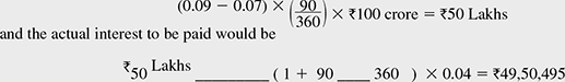
In this illustration, the firm pays fixed and receive floating rate as a hedge since it wanted to avert loss in a scenario where interest rates were rising. (We can see that this is very similar to a short futures position.)
Similarly, Bank B would take its position as a hedge when interest rates are expected to fall. This is similar to a long futures position.
Risks Involved in Using FRAs
- Their resemblance to forward contracts implies that FRAs are also subject to credit risk. There is a possibility that the counterparty may default when payment under the FRA is due.
- The transaction depends on the integrity and creditworthiness of counterparties, and this has to be gauged by the parties themselves, without the guarantee or backing of exchanges/clearing houses as in the case of futures.
- In practice, it may be difficult to find the counterparty that can take exactly the opposite position. There may also be disagreement between counterparties on the settlement date or the notional principal amount, and so on. This may lead to higher transaction costs as well.
- Relative to other types of IRDs, FRAs are not very liquid. If one of the counterparties wants to exit the contract midway, compensation needs to be paid, as the contract has to be assigned to another party.
Interest Rate Options
Like all financial derivatives, interest rate options derive their value from an underlying security, which, in this case, would typically be a reference interest rate or an interest rate index. Interest rate options provide protection against adverse market moves, while enabling the holder to still benefit from favourable shifts in the market. Box 12.8 briefly explains the concept of ‘financial options’ and Box 12.9, the difference between options, forward and futures contracts.
To illustrate, assume that Bank A has lent ₹100 crore based on a floating rate. The rate is set at say LIBOR + 3%. Bank A is happy when LIBOR is increasing—but also wants to protect itself against drops in LIBOR. The level at which the bank would like to cover itself is, say, 9 per cent total. In other words, it wants to protect itself against LIBOR falling below 6 per cent.
The solution is to buy an ‘interest rate put option’. This contract will specify a notional amount (say ₹100 crore − the loan amount), the strike rate (6% LIBOR) and a maturity date on which the option would expire.
Let us assume LIBOR does drop to 4 per cent. Bank A will exercise the option, and receives a payment from the option issuer as follows:
That is, the difference between strike rate (6 per cent) and actual rate (4 per cent) times ₹100 crore, which equals ₹2 crore.
Bank A will also receive from its borrower 7 per cent (LIBOR—4% + 3%) times ₹100 crore. In effect, the bank has received the desired minimum return of 9 per cent on ₹100 crore, of course, it would have had to pay a fee to the option issuer in return for the protection provided.
Similarly, Bank A could have entered into an interest rate call option to hedge against interest rate increases on its floating rate deposits. Assume that on a ₹100 crore deposit, the bank does not want to pay more than 9 per cent (LIBOR +3%). If the LIBOR does increase to 7 per cent, Bank A will have to pay its depositor ₹10 crore by way of annual interest. Bank A will now exercise the call option, and the option issuer pays (7% − 6%) × 100 crore or ₹1 crore, which taken with the ₹9 crore (9 per cent) the bank was willing to pay, would satisfy the depositor. If interest rates start dropping, the bank would not exercise the option and would still benefit since it has to pay less to the depositor.
Note that in the above example, we have made the simplifying assumption that all payouts are after a year.
Caplets and Floorlets In financial terms, the call option described above is called a ‘caplet’ and the put option, a ‘floorlet’. The reason for the nomenclature is clear—a ‘caplet’ protects the bank against large increases in interest rates—it has effectively set a ‘cap’ on the bank’s interest outgo. Similarly, the floorlet has ensured that drops in interest rate do not eat into the bank’s earnings—it has effectively guaranteed a minimum level of income floor for the bank.
BOX 12.8 FINANCIAL ‘OPTIONS’—THE BASICS
An option is a private contract between two parties, in which the holder has (a) the right to buy an underlying asset at a predetermined price, k, by a specified date, t, or, (b) the right to sell an underlying asset at a predetermined price, k, by a specified date, t.
Options form a unique type of financial contract since they give the buyer of the option the ‘right’, but not the ‘obligation’, to exercise the option. In other words, the buyer uses the option only if it benefits him/her; otherwise, the option can be discarded or allowed to lapse.
Some basic terminologies used in financial options are as follows:
- The writer of the option is the seller of the option. The writer grants the right to buy or sell the underlying security to the buyer of the option.
- The holder of the option is the buyer of the option. The buyer has the right to buy the underlying security from or sell it to the writer on or before a specified date.
- The option with a right to buy the underlying security is the call option.
- The option with a right to sell the underlying security is the put option.
- The option price or option premium is the sum of money paid by the buyer of the option to the seller for gaining the right under the option.
- The predetermined price at which the underlying security may be bought or sold is the strike price or exercise price.
- The date specified in the contract is the exercise date or expiration date or maturity. After this date, the option contract becomes void.
- The underlying assets in financial options can include stocks, stock indices, foreign currencies, debt instruments, commodities and futures contracts.
- Options can be categorized according to when the buyer may exercise the option. American options can be exercised at any time up to (and including) the expiration date. European options can be exercised only on the expiration date. (It is to be noted that the terms ‘American’ and ‘European’ do not refer to the location of the option or the exchange)
- The value of a call option on expiration date would not be known before expiration. If this value s is greater than the exercise price, k, the call is said to be in the money. If s is smaller than k, the call is out of the money.
- The circumstances that establish the value of a put option are the opposite of those for a call option. The put option gives the holder the right to sell the asset, and hence it would not make sense for the holder to sell if the price at expiration s is greater than the exercise price k. In other words, the put option is worthless if s exceeds k. In this case, the put option is out of the money. The put option will be in the money if s is less than k.
Valuing the option
Consider the following example. An American call option contract on shares of firm V, has an exercise price of ₹600. Assume that the share sells at ₹700 today, a few days prior to expiration. The option price in this case is likely to be above ₹100, since investors would rationally pay more than ₹100 in the expectation that the share price would rise above ₹700 in the forthcoming days prior to expiration. (It is to be noted that the option cannot sell below ₹100 since this would result in ‘arbitrage profit’—that is, profit from a transaction that has no risk or cost, but aimed at taking advantage of the price differential for the same stock in two different markets. If arbitrage profit did happen, the excess demand for this call option would quickly force the price to rise to at least ₹100.). However, the option price for buying the share cannot have a greater value than the market price of the share itself, since it would not make sense to buy a share with a call option, when the share itself can be purchased at a lower price.
It is, therefore, evident that the call option value will be bounded as follows—the upper bound of the call option will be the price of the stock itself s, and the lower bound for the option will be the difference between the stock price and the exercise price (s – k).
Therefore, the following factors can be seen to determine the value of a call option—(a) exercise price (the higher the exercise price, the lower the value of the call option), (b) stock price (the higher the stock price, the more valuable the call option), (c) interest rate (the higher the interest rate, the more valuable the option), (d) expiration date, and (e) the variability of the underlying asset (the greater the variability of the underlying asset, the more valuable the call option). The value of a put option is determined by the same factors operating in the opposite direction.
If both the call and put options share the same expiration date and exercise price, it is seen that a relationship evolves between the prices at the time of the original position, which can be expressed as follows:
The above expression is commonly called the ‘put call parity’
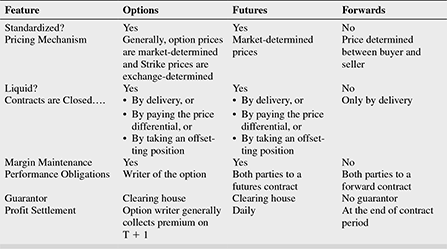
Interest Rate Caps and Floors In practice, it may so happen that both the depositor and borrower may want to invest/borrow for periods longer than a year, say, 9 years. In this case, the bank will have to buy a series of caplets and floorlets for 1, 2, 3 years and so on. To simplify the procedure, the option instruments of different maturities can be bundled together as one instrument.
A bundle of interest rate caplets with the same strike rate but different maturities is called an ‘interest rate cap’. Similarly, a bundle of interest rate floorlets with the same strike rate and different maturities, is an ‘interest rate floor’
What do interest rate ‘Caps’ do? They protect the bank (or the holder) against rising interest rates on its liabilities in the short term. If the underlying interest rate exceeds a specified ceiling rate, the option issuer (called ‘cap issuer’) makes payment to the bank. The payment will be equal to the difference between the actual rate and the strike rate times the notional amount specified in the option contract.
What do interest rate ‘Floors’ do? They protect the bank from interest rates falling below a desired minimum, the strike rate. The payment by the option issuer for a floor is determined by the difference between the strike rate and actual rate times the notional amount.
A series of payments—caplets or floorlets—are made during the period of the contract.
The benefits of buying caps or floors are similar to those of buying any option. The bank that buys a cap can set a maximum (cap) rate on its cost of borrowed funds. It can also convert a fixed rate liability to a floating rate liability. In the process, it gets protection when rates are increasing, and retains the benefits in case rates fall. The cost of such protection would be the upfront premium that the bank pays the option issuer. In an environment where interest rates are rising, such premiums could be quite high. Similarly, when interest rates are expected to fall, the premium for buying interest rate ‘floors’ would be high.
Interest Rate ‘Collars’ In some cases, to compensate for the premium paid on ‘caps’ and ‘floors’, banks buy interest rate ‘collars’ or ‘reverse collars’.
When a bank purchases a ‘collar’, it is actually simultaneously buying an interest rate cap and selling an interest rate floor—the notional amount, maturity and index being the same. In buying a cap, the bank’s objective is to protect against rising interest rates. By simultaneously selling the floor, the floor rate being set below the cap rate, the bank generates premium income.
Buying a collar would, therefore, be beneficial to a bank as long as interest rates are rising. When the actual interest rate (the index) rises above the cap (strike rate), the bank receives payment from the option issuer. If the actual index falls below the floor, the bank, as the collar buyer, would have to pay the option issuer the difference between the strike rate (floor) and the actual rate.
Therefore, a collar creates a ‘range’ within which the buyer’s effective interest rates fluctuate.
Theoretically, it is possible to have a ‘zero cost collar’, where the cap and floor rates are so chosen that the premiums are equal, and there is no net premium outgo for the bank buying the collar.
When the bank wants to protect its earnings from assets when interest rates are falling, it buys a ‘reverse collar’. This is the opposite of a collar, and refers to simultaneously buying an interest rate ‘floor’ and selling an interest rate ‘cap’. The motivation for selling the cap is to compensate for the cost of buying the floor. When the actual rate falls below the floor, the bank, as the buyer of the ‘reverse collar’, receives payment from the option issuer. However, if interest rates rise above the cap, the bank will have to make cash payment to the option issuer. The net result is that the bank’s interest rate fluctuates within a range.
Banks can also construct ‘zero cost reverse collars’ where they can find floor and cap rates with identical premiums that provide an acceptable interest rate band.
How do banks choose between swaps, caps and floors and collars?
Illustration 12.10 serves to clarify.
ILLUSTRATION 12.10
Assume that Bank A is asset sensitive, and a fall in interest rates would lead to a fall in NII. Also assume that the bank holds ₹100 crore of loans priced at prime +2%. The loans have been funded with a 5-year deposit costing 6.10 per cent to the bank. Interest rates may rise or fall over the next 5 years, but the bank wants to guard against a fall since its loans are at floating rate.
The bank is evaluating the following three alternatives:
- It can enter into a plain interest rate swap, to pay LIBOR and receive a fixed rate,
- It can buy an interest rate floor, or
- It can buy a reverse collar.
All the alternatives are evaluated considering the following assumptions:
- The current loan rate has been assumed at 10 per cent, and the cost of deposit at 6 per cent.
- The loan rate is assumed to be linked to the bank’s prime rate, and hence moves up or down based on prime rate changes. For ease of calculation, the rate movements have been assumed at 100 bps.
- LIBOR is assumed at 6 per cent and movements at 100 bps.
Case 1 Interest Rate Swap—The bank pays LIBOR and receives 6.05 fixed.
| Base case LIBOR 6% | Interest Rates Fall by 100 bps LIBOR 5% | Interest Rates Rise by 100 bps LIBOR 7% | |
| NII | |||
| Loan interest earned | 10% | 9% | 11% |
| Cost of deposit | 6.10% | 6.10% | 6.10% |
| Spread | 3.90% | 2.90% | 4.90% |
| Interest rate swap flows | |||
| Fixed-inflow | 6.05 | 6.05 | 6.05 |
| LIBOR (floating)—outflow | 6 | 5 | 7 |
| Spread | 0.05 | 1.05 | – 0.95 |
| Total spread | 3.95 | 3.95 | 3.95 |
Case 2 Buy 6% Floor on LIBOR—The bank receives when LIBOR falls below 6%. For this, it has to pay a fee of 0.2% per year
| NII | |||
| Loan Interest earned | 10% | 9% | 11% |
| Cost of deposit | 6.10% | 6.10% | 6.10% |
| Spread | 3.90% | 2.90% | 4.90% |
| Interest rate floor flows | |||
| Payout—inflow | 0 | 1 | 0 |
| Fee—outflow | 0.2 | 0.2 | 0.2 |
| Spread | – 0.2 | 0.8 | – 0.2 |
| Total spread | 3.7 | 3.7 | 4.7 |
Case 3 Buy Reverse Collar-Buy 5.5 % Floor On Libor, Sell 6.5% Cap On Libor-The bank will pay when LIBOR exceeds 6.5%, and will receive when LIBOR falls below 5.5%. The premium will be 0.05%.
| NII | |||
| Loan interest earned | 10% | 9% | 11% |
| Cost of deposit | 6.10% | 6.10% | 6.10% |
| Spread | 3.90% | 2.90% | 4.90% |
| Reverse collar flows | |||
| Payout-inflow | 0 | 0.5 | – 0.5 |
| Fee-inflow | 0.05 | 0.05 | 0.05 |
| Spread | 0.05 | 0.55 | – 0.45 |
| Total spread | 3.95 | 3.45 | 4.45 |
Thus, it is evident that all three alternatives perform efficiently, and decision of the bank to prefer one instrument over the other depends on the objectives for which protection is sought for, and the risk appetite of the bank.
Interest Rate Guarantees
Interest rate guarantees (IRGs) are very similar to interest rate options, the only difference being that the hedging period is restricted to 1 year. In place of the option premium, the guarantor receives a guarantee commission.
Swaptions
Our earlier discussion introduced plain vanilla interest rate swaps. Financial innovation and the need for prudent risk management at least cost have been instrumental in expanding the types of instruments available for mitigating risks, as well the nature of their application.
One such innovation is the ‘swaption’, which as the name suggests, is an option on a swap. The holder of a swaption has the option of entering into a swap contract at a predetermined fixed rate during the agreed period. For example, a 1-year swaption gives the holder the right to purchase a swap within the year. However, at the end of the year, there is no obligation to enter into the swap arrangement. It follows that a receiver of a swaption has the right to receive the fixed rate, and a payer of a swaption has the right to pay the fixed rate.
As with options (see Box 12.8), there are ‘calls’ and ‘puts’ in swaptions as well. The buyer of a put or call swaption pays a premium to the option issuer.
A ‘call swaption’ gives the holder the right to enter a swap contract where the holder pays a fixed rate and receives a floating rate. The holder also has the right to terminate the swap after a fixed period of time. Similarly, a ‘put swaption’ gives the holder the right to put the security back to the issuer even before maturity. In this case, the party receiving the fixed payment has the option to terminate the swap after a certain period, which option is likely to be exercised when interest rates are increasing.
A ‘callable’ or ‘puttable’ swap is essentially a swap with an embedded option. Since a swaption effectively permits parties to terminate the swap, it is also referred to as a ‘cancellable’ or ‘terminable’ swap.
Swaptions have found applications in areas such as (a) anticipatory financing, (b) managing future borrowing costs and (c) changing existing swap terms. For example, if a borrower being charged floating rates fears that interest rates will not fall in future, he can reduce funding cost by selling a receiver swaption. Similarly, a borrower who is not sure if he wants to lock in interest rates for 1 year, can delay the decision by buying a payer swaption.
Arbiloans
Another recent innovation is ‘Interest Arbitrage financing’, also called ‘Arbiloans’. These are useful to multinational corporations operating in high interest rate and low interest rate countries. Let us assume a subsidiary of this corporation is operating in a low interest rate country. The subsidiary borrows locally at the lower rate, converts into parent’s home currency at spot rates, and lends the amount to the parent. The parent company guarantees to repay the principal along with interest, while hedging against adverse exchange rate movements.29
Derivatives Market Growth—The Issues
The market for interest rate and other derivative products is growing rapidly. Box 12.10 examines whether use of these risk management tools could create fresh risks for banks. Box 12.11 outlines the accounting standards adopted by the international community to make derivative transactions and their risks more transparent to the public.
BOX 12.10 ARE DERIVATIVES RISKY FOR BANKS?30
At around USD 344 trillion,31 the notional amount of interest rate derivatives outstanding globally at the end of September 2009, may appear daunting. However, considering that this position had touched a peak of USD 600 trillion in 2007, and then plunged to a low of USD 294 trillion at the end of June 2009, the position in September 2009 appears to indicate stabilizing financial market conditions. However, we have to understand how risky this position is, and whether it renders the world’s financial system vulnerable to further shocks!
While the notional amount is a proxy for the amount of derivatives activity, it does not reflect the riskiness of the activity. In the case of derivatives, the notional amount is seldom at risk of loss. It is the derivatives investor who is at risk of loss from changes in prices of or rates earned on the financial assets that the notional amount represents.
There are three broad kinds of derivative activities that banks involve in—hedging, dealing and speculating,
When used for ‘hedging’, a derivative is used to mitigate the risk associated with an existing balance sheet position. Banks use ‘dealing’ in derivatives to earn fees—the bank essentially functions as an intermediary and makes contracts available to customers for a fee. In turn, the bank may enter into offsetting positions with other customers or manage derivative risk in other ways. ‘Speculating’ in a derivative transaction would have the objective of earning profits from expectations about derivative price movements that differ from market expectations.
Most banks are involved in derivatives transactions as only ‘hedgers’ or ‘dealers’. It is not easy to determine the extent of speculation—one, because speculation is not reported, and two, since speculative type risks could arise from certain dealer activities.
The three prevalent types of derivatives contracts banks enter into or facilitate are (a) interest rate derivative contracts, (b) foreign exchange derivative contracts and (c) equity, commodity and other types of derivative contracts.
Interest rate derivative contracts, which form the bulk of contracts banks enter into, are relatively less risky than other derivative types, say equity derivatives. This is because the magnitude of changes in short-term benchmark rate such as LIBOR is likely to be significantly lower than the changes in the stock market composite index. Hence, losses on the interest rate contract are more likely to be a small percentage of the notional amount. Exposures to equity or commodity for the same period are more likely to be a significant percentage of the notional value.
The risk in derivative activities also varies according to the objective for which the contracts have been created. Hedging, by definition, is a risk mitigating activity, and as already discussed, the risk of losses could be lower relative to other derivative activities. Derivative dealers are exposed to similar risks as hedgers, as well as ‘operational risk’ as a result of the huge volume of derivatives activity they undertake. A speculative objective, on the other hand, can lead to very high risk exposures, highly leveraged with minimum capital investment.
The risk of hedging primarily arises from the extent of variation in the value of the derivatives contract in relation to the value of the hedged item. This relationship is called ‘correlation’. Accordingly, the least risky hedge exhibits relative price movements between the derivative value and the hedged item, which have been consistent over time and are close to completely opposite—implying that price movements have tended to offset one another over time.
Research by the Federal Deposit Insurance Corporation (FDIC)32 reveals that most banks in the US that use derivatives hold them for hedging purposes. However, in terms of dollar volume, these hedging-related holdings amount to less than 0.5 per cent of the total notional amount. More noteworthy is the fact that almost 90 per cent of the derivatives held for hedging purposes are interest rate contracts—indicating that banks prevalently use derivatives to mitigate interest rate risk. More recent trends seem to support this observation—the BIS quarterly review quoted above estimated (page 24) the total turnover in derivatives markets at the end of September 2009 at USD 426 trillion (indicating a rebound from USD 366 trillion the previous quarter). Of this amount, about 80 per cent (USD 344 trillion) constituted interest rate derivatives.
The FDIC report also opines that it would be difficult to isolate and measure derivatives risk from total trading risk since most of the leading banks conduct derivatives activities as part their total trading activities. Even if a bank is speculating in derivatives, it occurs within the trading portfolio and hence cannot be measured separately.
Dealer banks face three critical risks from derivatives activities—market risk, credit risk and operational risk.
Market risks for banks in derivative activities
Banks use a combination of (a) matched trading, (b) market making and (c) positioning, while engaging in customerrelated trading activities.
In matched trading, the dealer bank enters into a trade with a customer, and then enters into an equal offsetting position with counterparty. Although the bank could succeed in eliminating its market risk, it retains the credit risk, both from the customer and the counterparty.
Market makers, on the other hand, are ready to enter into certain contracts without an offsetting transaction. Though this approach exposes the bank to market risk, the bank compensates for the market, credit and liquidity risks through the intra day bid/ask spread, and rake in additional profits through intra day positioning. Generally, market makers try to offset intra day risks at the end of the trading day.
Positioning exposes the bank to speculation-like risks. Here, the bank takes on a transaction without establishing an offsetting position (called an ‘open position’), probably expecting favourable market movements, or to maintain an inventory of financial instruments that customers may demand. These positions, unlike the market making positions, can be carried over for more than a trading day.
Hence, the magnitude of derivatives market risk in banks would bear a relationship to the extent to which the bank indulges in matched trading, market making and positioning.
Credit risks for banks in derivative activities
Even where market risk is under reasonable control, credit risk could arise out of current exposure or potential future exposure.
Current exposure represents the fair value33 of the bank’s derivative contracts with a positive value, and the ‘exposure’ is determined by the cost of replacing the contract in the event of non-performance by the counterparty.
Potential future exposure is more difficult to estimate, since it represents an estimate of the contract’s replacement value.
Credit risk is generally mitigated by (a) netting positions open to the same counterparty, (b) carefully selecting creditworthy counterparties, and (c) ensuring that the counterparty is also hedging its earnings with derivatives.
Operational risks for banks in derivative activities
The largest derivative losses documented so far can be attributed to operational—arising from banks circumventing risk management controls. Since operational risks are typically expected to increase with the growth in volume of transactions, each derivative contract must be properly executed and managed throughout the contract period.
More research on the riskiness of derivatives
More new research on the benefits of derivative contracts serves to corroborate the arguments in the foregoing paragraphs. According to a University of Michigan study34 of interest rate risk management in the banking sector, derivatives allow banks to maintain smooth operating policies and avoid unwanted costs, even when faced with external shocks.
BOX 12.11 ACCOUNTING FOR DERIVATIVES—INTERNATIONAL PRACTICES AND THE POSITION IN INDIA
In the previous chapter we learnt of the proposed move to IFRS 9 and its intended treatment of Expected Credit Losses. The following paragraphs elucidate on the role of IFRS in general, and in particular, accounting for derivatives
Given the nature and risks of banks’ involvement in derivatives, there is a growing concern that the present disclosures being made by banks in respect of their derivatives exposure need considerable transparency and fine tuning. In addition, international accounting practices are at present moving towards standardization and convergence in respect of all financial instruments including derivatives.
Background—International financial reporting standards and the international accounting standards
The International Accounting Standards Board (IASB) is an independent private sector body established to develop and approve international financial reporting standards (IFRS). The IASB replaced the International Accounting Standards Committee (IASC) in 2001. Now IASB functions under the oversight of the International Standards Committee Foundation (IASCF), an independent non-profit foundation created for this specific purpose. An International Financial Reporting Interpretations Committee (IFRIC) develops and solicits comments on the standards developed by the IASB.
IFRS is used in a narrow as well as broad sense. In the narrow sense, IFRS is the new set of numbered pronouncements being issued by the IASB, as distinguished from the IAS series issued by its predecessor, the IASC.
In the broad sense, IFRSs refer to the entire body of IASB pronouncements, including standards and interpretations approved by IASB, IASs and others.
What are IFRS standards?
IFRS Standards constitute a globally recognised set of standards for the preparation of financial statements by business entities. IFRS Standards prescribe:
- the items that should be recognised as assets, liabilities, income and expenses;
- how to measure those items;
- how to present them in a set of financial statements; and
- related disclosures about those items.
Table 12.5 shows the IFRS standards as of April 2017
TABLE 12.5 IFRS STANDARDS – UPTO APRIL 2017 (WITH YEAR OF ORIGINAL ISSUE OR MAJOR AMENDMENT)

In 2015, the IFRS for Small and Medium sized entities, (IFRS for SMEs) was released by the Special Group for SMEs constituted by the IASB
The International Accounting Standards (IAS) run from IAS 1 to IAS 41. These have been issued during years ranging from 1987 to 2008. Some of the IAS provisions are being progressively replaced by IFRS. Significantly, IFRS 9 dealing with financial instruments, replaces IAS 39. These standards were set by the IASB’s predecessor, the IASC.
Additionally, IFRIC interpretations IFRIC 1 to 21 have also been issued by the Standards committee.
Adoption of IFRS standards
IASB surveyed 150 countries and other jurisdictions around the world, which together represent 98% of the world’s Gross Domestic Product (GDP), in respect of the extent of adoption of IFRS standards. The results were published on the IFRS website, and in the Pocket guide to IFRS standards: the Global financial reporting language, 2017.
Some of the key findings are listed below:
- The authorities in 142 (out of 150) countries have made a public commitment to IFRS standards as the single set of global accounting standards
- Of the 150 countries, 126 require IFRS standards for all or most domestic publicly accountable entities such as listed companies and financial institutions.
- All 31 members of the European Union require IFRS standards for all European companies whose securities trade in a regulated market
- Nine countries use national or regional standards – Bolivia, China, Egypt, Guinea-Bissau, India, Macao, Niger, the United States and Vietnam
The USA
Effective January 2001, the Financial Accounting Standards Board (FASB) of the US issued FASB 133—Accounting for Derivative Instruments and Hedging activities.
Both IAS 3935 and FASB 133 require that all derivatives, including hedges, be recognized on the banks’ balance sheet at their ‘fair value’, defined as ‘value at which an asset could be exchanged or a liquidity settled between knowledgeable, willing parties in an arm’s length transaction’.
We have seen that there are three broad types of derivatives contracts, classified according to objective—hedging, dealing and speculation. FASB 133 differentiates between hedging and speculative contracts, and sets forth three types of hedging relationships: (a) fair value, (b) cash flow, and (c) foreign currency.
A fair value hedge is a derivative contract entered into as a hedge against possible changes in the bank’s balance sheet asset and liability values. The gain or loss in net income is recognized in the period of change together with the offsetting gain or loss on the hedged item attributable to the risk hedged. The effect of the accounting is to reflect in earnings the extent to which the hedge is not effective in achieving offsetting changes in fair value.
A derivative contract entered into as a cash flow hedge seeks to hedge the variations in cash flows of a forecasted transaction. A ‘forecasted transaction’ is that a bank expects to occur, but is not obligated to carry out in the course of its normal operations. The primary purpose of a cash flow hedge is to link a hedging instrument with a hedged item whose changes in cash flow are expected to offset each other. The gain or loss in such transactions are initially reported outside the profit and loss account, and subsequently included in earnings when the forecasted transaction actually affects the earnings. The ineffective portion of the gain or loss is immediately reported in earnings.
In the case of a hedging contract entered into to cover the foreign currency exposure, the gain or loss is reported outside the profit and loss account. The accounting for a fair value hedge described above applies to a derivative designated as a hedge of the foreign currency exposure of an unrecognized firm commitment or an available-for-sale security. Similarly, the accounting for a cash flow hedge applies to a derivative designated as a hedge of the foreign currency exposure of a foreign-currency-denominated forecasted transaction.
For a contract not designated as a ‘hedging contract’, gain or loss is recognized in the period of change.
The bank applying the hedge accounting standards is required to determine, even at the inception of the contract, the method it will use to assess the effectiveness of the derivative instrument. The method adopted should be consistent with the bank’s overall approach to risk management.
However, the financial crisis of 2007 has prompted the FASB to introduce, effective November 2008, a new rule—FAS 161. The new rule requires the mark to market value of derivatives and their gains and losses to be shown in a table in company financial statements. The implication is that investors, regulators and other stakeholders would now have more information to estimate how complex derivatives and hedges affect companies’ financial statements.
FAS 133 is non (Since 2013) codified in ASC 815 under US GAAP. An update by FASB on June 22, 2017, shows the progress made in aligning the existing hedge accounting standards with IFRS 9.
The UK
In 1998, the Accounting Standards Board (ASB) published Financial Reporting Standards (FRS) 13, ‘Derivatives and other financial instruments: Disclosures’, which became effective March 1999. The standards have laid down the requirements for disclosures of a bank’s policies, objectives and strategies in using financial instruments, their impact on its risk, performance and financial condition, and details of how risks are managed.
In addition, Statement of Recommended Practice (SORP) supplements accounting standards. The latest version of the SORP on derivatives, issued in 2001, aims to ensure that derivatives held for trading purposes are measured at fair value. ‘Fair value’ is the amount at which the instrument could be exchanged in an arm’s length transaction between informed and willing parties. All fair value calculations should also take account of counterparty credit quality, market liquidity, closeout costs and other administrative costs. Changes in fair value should be recognized in the profit and loss account immediately. The fair value of trading derivatives, where positive, should be included in ‘other assets’ on the bank’s balance sheet, while the negative values should be included under ‘other liabilities’.
Derivatives classified as ‘non-trading’ transactions should be measured on an accrual basis, equivalent to that used for the underlying asset, liability position or cash flow.
FRS 102 the current accounting standard for hedge accounting is proposed to be modified and converge to IFRS 9.
Position in India
The Institute of Chartered Accountants of India (ICAI) has committed to the convergence of IASs and the IFRS from 1 April 2011. The ICAI has also issued Accounting Standards (AS) 30, 31.and 32 which incorporate the norms for recognition and measurement, presentation and disclosure of all financial instruments in line with IAS 32, 39 (to be replaced by IASB) and IFRS 7. The Companies Act 2013 contains many requirement aligned to IFRS. The government has implemented an Indian version of IFRS (Ind-AS) from April 2015. The previous chapter provides a brief description of Ind AS and its features.
Basel Committee’s guiding principles for replacement of IAS 39 (August 2009)
In response to the recommendations made by the G20 leaders at the April 2009 summit, the Basel Committee welcomes the replacement of IAS 39, provided the new standard avoids undue complexity, and takes into account the lessons from the financial crisis of 2007. IAS 39 will be superceded by IFRS 9 (Financial Instruments).