
SECTION V
LIQUIDITY RISK MANAGEMENT AND BASEL III
The financial turmoil of 2007 has once again underscored the importance of liquidity to the functioning of both the financial markets and the banking sector. A cataclysmic change from buoyant, liquid markets just before the crisis, to an extended period of illiquidity put the global banking system under severe stress. In February 2008, the Basel Committee noted that many banks had failed to follow some basic principles of liquidity management during times of abundant liquidity. In its paper titled ‘Liquidity risk management and supervisory challenges’,36 the Basel committee pointed out that:
- Most of the banks which exposed themselves to severe liquidity risks did not have the requisite framework to support the risks inherent in individual business lines or products, and, therefore, did not align the risks to the banks’ own risk tolerance.
- Many banks did not account for the ‘unlikely’ event of a large part of their contingent liabilities having to be funded all at once.
- To many banks the kind of severity or duration of the liquidity crisis (as it materialized later) seemed a remote possibility. Hence, these banks did not conduct stress tests to factor market wide liquidity strain and disruptions.
- Even where contingency funding plans were made, they were not related to results of stress tests, or did not factor in the possible drying up of some potential funding sources.
Simply stated, liquidity is a bank’s ability to generate cash quickly and at a reasonable cost. Liquidity risk is the risk that the bank may not be able to fund increases in assets or meet liability obligations as they fall due without incurring unacceptable losses. The problem may lie in the bank’s inability to liquidate assets or obtain funding to meet its obligations. The problem could also arise due to uncontrollable factors such as market disruption or liquidity squeeze. Figure 12.3 illustrates how a bank’s inability to generate cash is a manifestation of more serious problems.
FIGURE 12.3 ANATOMY OF LIQUIDITY RISK
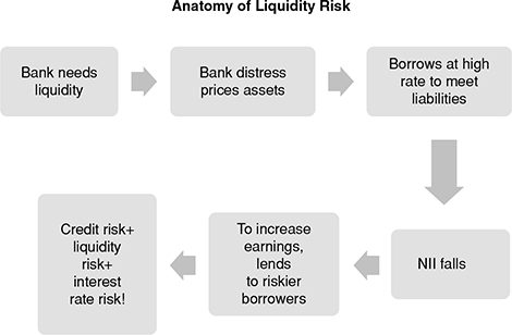
Liquidity problems can have an adverse impact on the bank’s earnings and capital, and, in extreme circumstances, may even lead to the collapse of the bank itself, though the bank may otherwise be solvent. A liquidity crisis in a large bank could give rise to systemic consequences impacting other banks and the country’s banking system as a whole. Liquidity problems can also affect the proper functioning of payment systems and other financial markets.
Sound liquidity risk management is, therefore, essential to the viability of every bank and for the maintenance of overall financial stability.
Recent trends in the liability profiles of banks pose further challenges to the industry and have made it increasingly important for banks to actively manage their liquidity risk. Some of these developments are: (a) the increasing proportion in bank liabilities of wholesale and capital market funding, which are more sensitive to credit and market risks; (b) the increase in off-balance sheet activities such as derivatives and securitization that have compounded the challenge of cash flow management; and (c) the speed with which funds can be transmitted and withdrawn, thanks to advanced technology and systems.
Why do banks need liquidity? They need liquidity in order to meet routine expenses, such as interest payments and overhead costs. More importantly, as financial intermediaries, they need liquidity to meet unexpected ‘liquidity shocks’, such as large deposit withdrawals or heavy loan demand. The most extreme example of a liquidity shock is a ‘bank run’.37 If all depositors attempt to withdraw their money at once, almost any bank will be unable to cover their claims and will fail—even though it might otherwise be in sound financial condition. However, individual institutions are rarely allowed to fail, thanks to the safety net existing in most countries in the form of deposit insurance, the central bank’s role as lender of last resort, and stringent capital requirements. Poor liquidity may, therefore, lead to outright failure only in exceptional cases. However, if a bank does not plan carefully, it may be forced to turn to high-cost sources of funding to cover liquidity shocks, thus cutting into profitability, and ultimately, into its very existence.
It is also evident that to manage liquidity risk at the basic level, two sources of liquidity are equally important. One is the liquidity generated from liquidation of assets—this implies that in an adverse situation the bank needs excess liquidity from assets. The second is the funding liquidity—raised through liabilities.
Of the four specific forms of risk that impact banking operation—credit risk, market risk, operational risk and liquidity risk—the first three have been extensively studied and commonly incorporated into existing capital allocation frameworks. However, at present, there is no technique for modelling liquidity risk that has wide acceptance.
Though its importance is well recognized, at present there is no coherent definition of liquidity risk. This comes as no surprise. The term liquidity is used across the market for different purposes, which means that liquidity risk itself is defined differently and depends very much on the context in which it is used. For example, one quite popular definition of liquidity risk is the risk that a particular banking asset cannot be converted into cash within a specific time frame and at a specific price level. It refers directly to the ‘liquidity’ of this particular asset and yet this risk impacts the bank. Literature contains many more such contextual definitions.
Again, no single balance-sheet category or ratio is sufficient to assess liquidity risk. It involves the entire balance sheet and off-balance sheet activity as well. Liquidity management is largely about being sure that adequate, low-cost sources of funding are available on short notice. This might include holding a portfolio of assets that can easily be sold, acquiring a large volume of stable liabilities or maintaining lines of credit with other financial institutions. However, this effort must be balanced against the impact on profitability. In general, more liquid assets earn lower rates of return and certain types of stable funding may cost more than those that are more volatile. A bank can be perfectly liquid by holding only cash as an asset, but this would be an unprofitable strategy because cash does not earn any income.
Why is it so difficult to isolate and study liquidity risk?
First, unlike the other three risks that are bank-specific, liquidity risk can transcend the individual bank—liquidity shortfall at a single bank can have repercussions on the entire banking system of a country.
Second, liquidity risk is partly confounded with market risk as depositor behaviour can arise from perceptions of the market state.
Third, liquidity risk cannot be eliminated or transferred, as can be done with say, credit risk. It has to be borne and managed by the individual bank.
Fourth, liquidity risk can occur in perfectly normal times—as when a large number of depositors withdraw their deposits within a short period of time—or in crisis times when the most severe outcomes can be expected.
Fifth, liquidity risk can affect both the profitability of the bank in the short term, as well as the very survival of the bank in the long term.
Sources of Liquidity Risk
A bank that plans well can anticipate many of its internal liquidity needs (such as funding loan growth, meeting depositor demands and paying operating expenses) and structure its balance sheet accordingly. If the bank knows its market, it can plan for many external events (such as seasonal borrowing patterns, deposit run-off and business practices requiring bank funds).
Apart from such anticipated needs, unforeseen events can have serious implications for a bank’s liquidity position. For example, frauds, natural disasters or resources malfunction could unexpectedly affect liquidity. Even with the most careful planning, banks need to maintain reserves of liquidity to sustain them when the unexpected occurs.
In general, factors that can influence bank liquidity include the following:
- Access to financial markets: Though most banks have some degree of access to financial markets for their funding requirements, larger banks have better access. Smaller banks may be equally creditworthy, but they lack the visibility and track record that larger banks enjoy in the markets. Tapping the market for funds could be expensive for smaller banks when the amount involved is not very large, since fixed transaction costs could be disproportionately high. Hence, smaller banks access the financial markets more infrequently or not at all.
- Financial health of the bank: Poor asset quality and earnings translate into adverse effects on a bank’s liquidity. Low quality of assets (or high level of non-performing/impaired assets) stifles earnings growth. Earnings represent a flow of funds to help meet liquidity needs. Thus, when earnings are low, cash availability is also low. Both factors in combination may place the bank’s solvency in doubt, which in turn, would deter potential lenders from providing funds.
- Balance sheet structure: Banks have to constantly trade off between liquidity and profitability. The most liquid bank would hold all its assets in cash or near cash investments, with most of its liabilities in stable core deposits. This bank can easily handle unexpected demand for funds and is not expected to face a liquidity problem in the foreseeable future. But such a bank would not be very profitable since its cash and near cash assets do not earn much income. The challenge for bank management is to, therefore, structure its balance sheet to earn a reasonable rate of return while maintaining a safe level of liquidity.
- Liability and asset mix: Many bank liabilities and assets have embedded options. Most short-term funding arrangements include option like structures where the provider of funds is permitted to withdraw on demand or at short notice. When such demands are large, the bank’s liquidity comes under severe strain.
- Timing of funds flow: There is continuous flow of funds in and out of a bank. Inflows happen primarily from principal and interest payments, asset sales, deposits and other borrowings, and non-interest income. Similarly, outflows typically occur from interest payments, addition to assets, such as loans and investments, deposit and borrowing repayments, and other overhead expenses. The inflows and outflows occur at various points in time, which fact is not reflected in the balance sheet. The timing difference in cash inflows and outflows has liquidity consequences.
- Exposures to off-balance sheet activity: Banks make various non-funded commitments to their customers, which could result in potential liquidity drain if the counterparties default. These commitments are not reflected on the balance sheet, but are shown as ‘contingent liabilities’. Further, a bank may have made loan commitments or unused lines of credit, which will have to be honoured on demand. Hence, the balance sheet alone may not convey the real picture of the liquidity strength of a bank.
- Impact of other risks: There is no single source for liquidity risk as there can be no single source for market or credit risk. Further, as we have seen earlier, any of the other risks can turn into liquidity risk—for example, credit risk affects cash inflow into the bank and, hence, affects liquidity. Similarly, volatility in market interest rates may affect the liquidity of a bank’s investment portfolio.
How to Measure Liquidity?
Historically, better practices for liquidity measurement and management focused on the use of liquidity ratios. These were static ratios, calculated from the bank’s balance sheet. The thinking then welcomed the use of more and more such ratios.
Use of these ratios presupposed that past performance was a realistic indicator of the future. Banks discovered that this assumption may not be valid in a dynamic environment when bank failures happened, triggered by liquidity risk. For example, a large regional bank in the US, Southeast Bank, used over 30 liquidity ratios to manage its liquidity. When it failed in 1991, the second largest failure of the previous two decades in the US, the reason cited was ‘liquidity risk’. It, therefore, became obvious that calculating more or different ratios was not the solution, since historical ratios, however well conceptualized, could say little about the future.
Now, better practices of liquidity measurement and management are evolving. These approaches focus on prospective liquidity, diversified funding and contingency planning. Such approaches can be used by all banks, irrespective of size and geographical area of operation.
The adage ‘you manage what you measure’ has been recognized by the regulators, as evidenced by the Basel III requirements for liquidity management, spelt out by the Basel Committee on Banking Supervision.38 It is noteworthy that the principles for liquidity management as spelt out by the committee have undergone substantial changes and have taken into account lessons from the financial crisis of 2007.
The Basel document of 2000 and 2008 specifically mentions the key areas (quoted below) where more detailed guidance has been provided39:
- The importance of establishing a liquidity risk tolerance.
- The maintenance of adequate liquidity, including through a cushion of liquid assets.
- The necessity of allocating liquidity costs, benefits and risks to all significant business activities.
- The identification and measurement of the full range of liquidity risks, including contingent liquidity risks.
- The design and use of severe stress test scenarios.
- The need for a robust and operational contingency funding plan.
- The management of intraday liquidity risk and collateral.
- Public disclosure to promote market discipline.
The Basel document mentions two kinds of liquidity risk—funding liquidity risk and market liquidity risk. It defines the two kinds of risk as follows: (page 1) ‘Funding liquidity risk is the risk that the firm will not be able to meet efficiently both expected and unexpected current and future cash flow and collateral needs without affecting either daily operations or the financial condition of the firm. Market liquidity risk is the risk that a firm cannot easily offset or eliminate a position at the market price because of inadequate market depth or market disruption.’ The guidance in the document focuses primarily on ‘funding liquidity risk’.
However, these two risks are not independent of each other. For example, under conditions of stress, investors in capital market instruments may demand higher compensation for increased risk, or simply refuse to lend. The need for funding liquidity may then increase, since the illiquidity in the market may make it difficult for banks to raise funds by selling-off assets.
In addition, Basel III has proposed liquidity coverage ratios described later in this section.
Modern Approaches to Liquidity Risk Management
It is evident that liquidity risk is closely linked to the nature of banking assets and liabilities. The assets and liability positions of a bank, in turn, are affected by the bank’s investment and financing decisions, irrespective of whether they have short- or long-term implications.
It follows that banks should be able to manage their liquidity position both on an everyday basis as well as in the long term, to ensure that liquidity risk is effectively mitigated. This implies that a bank should preferably have two approaches to managing short-term and long-term liquidity.
Choosing the appropriate approach would depend on the bank management’s ‘liquidity policy’. What is important here is that board-approved policies address liquidity in some manner and that the board monitors both compliance with these policies and the need to change them as necessary.
The Liquidity Policy Similar to a bank’s ‘loan policy’, which we saw in an earlier chapter, many banks have the practice of formulating a ‘liquidity policy’ for the bank.
Policies on liquidity are likely to vary from bank to bank based on individual operating environments, customers and needs. Also, policies will be subject to change over time as a bank’s situation and environment change.
An illustrative list of typical features of a sound liquidity and funds management policy and some symptoms of potential liquidity problems are provided in Annexure III.
It should be noted here that the involvement of a bank’s top management is extremely important in the process of ‘liquidity risk management’.
Approach to Managing Liquidity for Long-Term Survival and Growth
Since the bank’s long-term survival and growth are the driving factors, this approach tries to mitigate long-term liquidity risk by strategically controlling the bank’s asset and liability positions. This could be achieved by (a) aligning the maturity of assets and liabilities so that cash flow timing risks are eliminated, or (b) diversifying the funding sources so that liquidity availability is ensured.
The alternative approaches prevalently used by banks are:
- Asset Management, and
- Liability Management.
Asset Management All bank assets are a potential source of liquidity. The asset portfolio of a bank can provide liquidity in the following circumstances—(a) on maturity of the asset; (b) on sale of the asset; and (c) the use of the asset as collateral for borrowing or repo transactions.
Typically, banks hold liquid assets such as money market instruments and marketable securities to supplement the conventional funding sources such as deposits and other liabilities. When the cash inflows from asset realization, either on maturity or through sale, are less than anticipated due to default risk or price volatility, the bank incurs liquidity risk. Similarly, secured funding, such as repos, may be affected if counterparties seek larger discounts on the collateral provided or demand better quality collateral. Additionally, concentrated exposure of the asset portfolio to specific counterparties, instruments, economic activity or geographical location, may heighten the level of liquidity risk.
We have seen in earlier chapters that the typical bank has very few fixed assets. Most of its assets are in the form of loans and investments. Though, theoretically, in an extreme situation, even the bank’s building can be sold to provide funds, banks generally use shorter-term or readily marketable assets for liquidity purposes.
Of course, when the bank needs cash, the best thing to have on hand is cash. That is the reason vault cash, deposits at banks and other cash items are considered a bank’s primary reserve. The problem with cash is that it does not earn a return. Therefore, banks often hold relatively little vault cash, keeping their liquidity reserves in assets that earn some interest.
We have also seen in an earlier chapter that many central banks insist on creating secondary liquidity reserve for banks through investing in approved securities. Securities can be liquidated quickly and at relatively little cost. Also, they provide interest income to the bank.
Secondary reserve securities used for asset management would typically exhibit the following characteristics: (a) they will be short-dated, with maturity periods below 1 year, (b) they will be high quality instruments with low default risk, (c) they will be highly marketable, and (d) have a low conversion cost.
For a bank resorting to ‘asset management’ as a strategy to mitigate liquidity risk, its investment portfolio is looked upon as a liquidity shock absorber. However, there is a trade off between asset liquidity and profitability for the bank, since short-term, liquid, risks-free assets yield relatively low returns.
How much of liquid assets should a bank maintain? The level of liquid assets is generally a function of the stability of the bank’s funding structure and the potential for rapid expansion of its loan portfolio. Generally, if a bank has stable sources of funds and predictable loan demand, a relatively low allowance for liquidity may be required.
However, it is prudent to maintain higher allowance for liquidity to offset the factors described in the following illustrative list:
- The potential customer has a wide choice for investment in alternative instruments, due to the highly competitive environment.
- Recent trends also show that large liability account inflows are substantially lower.
- The bank’s access to the capital market is limited due to various reasons.
- A sizeable portion of the loan portfolio consists of large impaired credits, with little potential for recovery.
- A sizeable portion of the loan portfolio consists of loans whose credit risk cannot be diversified through credit risk transfer or loan sales.
- A substantial amount of lines of credit and commitments already sanctioned are unused, and could be potential outflows at any time.
- The bank’s credit exposure is concentrated in one or more industries with present or anticipated financial problems.
Hence, to balance liquidity and profitability, management must carefully evaluate the full return on liquid assets against the expected (risk-adjusted) return associated with less liquid assets. Adverse balance sheet fluctuations may lead to a forced sale of securities, in which case the potential higher income from securities may be lost.
Liability Management Liability management has been popular with larger banks since 1960s and 1970s. As the name suggests, the strategy focuses on sources of funds to mitigate liquidity risk.
Contrary to the practice in ‘asset management’, where surplus funds of the bank are parked in cash or near cash assets like readily marketable securities, a bank resorting to ‘liability management’ would invest its surplus funds in long-term assets. When there is a need for liquidity, the bank raises funds from external sources. Typically, the ‘liability-managed’ bank would manage its deposits and other borrowings judicially to meet its funding obligations.
In almost all banks, deposits constitute the largest component of liabilities. Of these, ‘core deposits’40 are generally the lowest-cost funding source because the presence of deposit insurance almost eliminates depositor concerns about the repayment of their funds.
Banks typically employ different liability funding strategies to manage liquidity risk. Those with large branch networks find it easier to garner relatively low-cost retail deposits. Banks concentrating on wholesale business may find borrowing in the money market the most efficient way of obtaining short-term liquidity. Others may issue medium-term certificates of deposit (CDs) or prefer term deposits with a spread of maturities to reduce liquidity risk.
Generally, banks that have a large and ready source of core deposits find liability management an easier task than those that must rely on more volatile, non-core deposits. Unfortunately, few banks have a large base of core deposits in the present competitive environment where investors are constantly seeking more profitable avenues to park their savings. Consequently, many banks now rely more heavily on non-core deposits and other non-deposit sources for funding. The greater volatility associated with these funds increases the rigour needed in a bank’s liquidity management.
The underlying implication of this approach is that a bank will not depend on its liquidity position for credit commitments, since it intends raising the required funds from external or market sources. While the approach would benefit large, growth-oriented, aggressive banks by way of higher returns, it also involves greater risk for the bank.
One risk would be the sustenance of high spreads—while the yields could be high, the cost of borrowing could also be high and in some cases, out of the bank’s control, since borrowing depends on market conditions.
The second would be the asset liability risk. Making long-term investments or loans also requires liabilities of matching maturity. It is likely that at the time the bank wants to source funds of a specific maturity, such sources may not be available, or available at a very high cost, or with embedded options.
The above factor would lead to a third risk—refinancing risk. If liabilities of shorter maturities are deployed in longer-term assets, the liability would fall due for payment before the asset flows come in completely. The bank would then have to seek more liabilities to match the remaining maturity of the assets. If interest rates are rising, there is likelihood that the new source of funds is priced much higher than the earlier one, which might render the transaction unviable.
A fourth risk—a critical one—cannot be ruled out. As the bank borrows more and more, it is vulnerable to credit risk. If a bank defaults on repayment of liabilities, it also runs a reputation risk.
Asset Management or Liability Management? Choosing between the strategies of ‘asset management’ and ‘liability management’ depends to a large extent on not only the size and nature of operations of a bank, but also expectations of how interest rates are going to move in the foreseeable future.
For example, consider a bank whose proportion of retail customers, both depositors and borrowers, is large. Though the amount per transaction, whether deposit repayment or loan disbursement, would be low, the volumes are likely to be large, and the payments would mostly be on demand. The surplus and deficits that arise on a periodic (depending on the liquidity planning horizon that the ‘liquidity policy’ has recommended) basis due to mismatch in cash inflows and outflows will have to be closely monitored. Surpluses, when they occur, will have to be accumulated carefully to take care of times of deficit, to ensure that the bank’s liquidity is not impaired. Instead of maintaining the surplus inflows in the form of cash, the bank would find it more profitable to invest them in short-term securities that can be liquidated at short notice to yield cash. Such a bank, therefore, would prefer the asset management strategy.
On the other hand, the large bank with a substantial proportion of wholesale customers, typically also has large volatile deposits as liabilities. The need for funds would arise in this case for payment of balances in demand deposit accounts and large volatile accounts, as well as for the expected and unexpected needs of its large borrowers. The bank is also likely to have good credit rating in the market due to its large-scale lending and investing activities. In the case of this bank too, periodic mismatches in cash inflows and outflows are likely to arise. However, this bank, unlike the predominantly retail bank discussed above, would be more likely to invest its surplus in long-term loans or investments. The deficits would be met by borrowing in the market, which is facilitated by its market reputation.
Due to the short-term investment strategy, the bank opting for asset management may have to forego higher yields. An alternative this bank has is to invest in long-dated securities and liquidate them in the secondary market as and when the need arises. However, the transaction costs and characteristics of the secondary markets will play a major role in deciding for this alternative. In any case, marketable securities that are relatively risk-free do not yield high returns.
On the other hand, the bank opting for liability management may be looking for higher returns, which do not come without the attendant risks. First, the bank will have to access various types of lenders and markets in its bid to raise funds. Interest rate fluctuations in any of the instruments or markets increase interest rate risk. Second, the bank will have to operate in well-organized markets with credit rating capabilities. A default by the bank in any of these markets would lead to a downgrade of the bank by the rating agencies, which, in turn, would push up the bank’s cost of borrowings. If the bank is not able to pass on the increased cost to its borrowers, its spreads weaken.
BOX 12.12 SOURCES OF CONTINGENT DEMAND FOR LIQUIDITY AND LIQUIDITY RISKS INHERENT IN OFF-BALANCE SHEET ACTIVITIES41
Off-balance sheet items, depending on the nature and size of transactions, can either supply or use liquidity. The following examples illustrate the effect of such items on a bank’s liquidity:
- It is common practice for a bank to obtain standby or committed facilities for funding from another bank or financial institution. However, the bank should be wary of restrictive covenants, if any, included in the facility agreement. Also, it should be able to test access to the promised funds regularly. Such testing would reveal the extent to which such facilities can be relied upon when the bank is in dire need or under stressed economic conditions.
- Unused loan commitments can draw on the bank’s liquidity at any time. The expected amount and timing of borrowers drawing on the unused commitments should be incorporated into the bank’s cash flows.
- Derivatives, options and other contingent items pose more challenges for liquidity risk management. The direction and amount of cash flows for such items will normally be affected by market interest rates, exchange rates and other special terms under the contract. For example, when a bank enters into an interest rate swap for paying a floating rate and receiving a fixed rate, it would receive a payment for the difference of the two rates only as long as the fixed rate is higher than the floating rate. In the event that interest rates increase, and the floating rate rises above the fixed rate, the bank will have to pay the difference of the two rates, thus incurring a cash outflow instead.
- Credit derivatives may have a liquidity impact that is often difficult to forecast. For example, assume that a bank enters into a credit default swap (CDS) to compensate a counterparty for its credit losses. The bank has sold credit protection, and, hence, exposed itself to a contingent liability, the cash flow of which cannot be easily determined.
- Special purpose vehicles (SPVs) can be a source or use of liquidity. Where a bank provides liquidity facility to an SPV under a contract or specific obligation, the bank’s liquidity would be affected by the illiquidity of the SPV. For example, if a securitization SPV is considered a source of funding by the bank, under stressed liquidity conditions, this source may be restricted or not available to the bank. Where the bank itself has sponsored or administered the SPV, liquidity pressures in either the bank or the SPV can trigger liquidity risks in both the entities.
- Foreign currency deposits as well as credit lines can be good sources of funding for banks. However, when market liquidity or exchange rates change suddenly, liquidity mismatches widen, which could even alter the effectiveness of the bank’s risk management/hedging strategies.
- Correspondent, custodian and settlement activities can lead to large cash flows, both on an intra day and overnight basis. Unexpected changes in these cash flows can impact the overall liquidity positions of banks, and the impact could be severe if banks fail to settle transactions on time.
Given the customized nature of the contingent contracts illustrated above, it is evident that triggering events for these contingent liquidity risks would be quite difficult to predict or model. Therefore, liquidity risk management in these cases would have to be based on analysis of assumptions and scenarios on the behaviour of both banks and counterparties under various conditions, even if there had been no adverse liquidity events in the past.
We have been discussing the risks arising from balance sheet assets and liabilities of banks. What are the risks inherent in off-balance sheet activities (contingent liabilities) of banks? Box 12.12 outlines some of the liquidity risks in off-balance sheet activities.
Approach to Managing Liquidity in the Short Term—Some Tools for Risk Measurement
A single measurement of liquidity risk rarely suffices in the short term. Banks basically use two kinds of tools used by banks to measure liquidity risk—forward-looking and retrospective—since sound liquidity management requires a complement of measurement tools.
Forward looking or prospective tools project funding needs in the foreseeable future—the planning horizon in such cases could range from daily to quarterly to half yearly and so on. When based on sound assumptions, these tools provide a good basis for liquidity planning in the short term.
Retrospective tools analyze historical behaviour and try to draw inferences for the future, though this may not necessarily prepare the bank for the future.
Some of the forward-looking tools prevalently used by banks include:
- Projected sources and uses of funds over the planning horizon.
- The working funds approach.
- Cash flow or funding gap report.
- Funding concentration analysis.
- Funds availability report.
A few typical retrospective tools include:
- Ratio analysis, and
- Historical funds flow analysis.
As opposed to managing the asset and liability positions for long-term liquidity management, the short-term approach manages the actual cash flows.
A few of the above approaches are discussed as follows:
1. The Working Funds Approach The working funds typically constitute bank’s capital and outside liabilities, such as deposits and borrowings as well as float funds.
In this approach, liquidity is assessed based on the working funds available with the bank. ‘Liquidity needs’ are typically estimated as a proportion of the working funds.
There are two ways in which a bank can estimate its liquidity requirements—one, as a proportion of total working funds. For example, the bank can decide to maintain 5 per cent of the total working funds as cash or near cash instruments for its liquidity requirements. A second approach is to segment the working funds and maintain separate liquidity limits for each segment.
In one commonly used segmentation approach, the bank classifies its liabilities based on their maturity profiles as follows:
- Owned funds of the bank are excluded from liquidity requirements since they have only residual claim
- Deposits and borrowings are segmented based on their withdrawal pattern.
- Volatile funds can be withdrawn at any time in the foreseeable future. These would generally include large amounts of funds parked by corporate houses and government bodies in short-term deposits and certificates of deposit. They call for almost 100 per cent liquidity allowance
- Vulnerable funds are those that can be withdrawn during the period for which liquidity planning is being undertaken. Most transaction deposits that are payable on demand fall under this category. Such deposits also call for almost 100 per cent allowance, or lower allowance depending on the bank’s risk appetite
- Stable funds have the least probability to be withdrawn during the period for which the liquidity planning is being done. These include the ‘core’ portion of savings deposits and time deposits not maturing during the planning period. The liquidity allowance for these funds would be much lower, based on the bank’s previous experience with the withdrawal pattern in such deposits.
- Float funds are similar to volatile funds, since these are mostly funds in transit or meant for a particular short-term purpose. Usually, a 100 per cent liquidity allowance is maintained for these funds, since they are payable on demand.
Based on the above allowances for components of its working funds, the bank would assess its desired liquidity levels at any point in time during the planning period. The bank, again depending on its risk-return characteristics, would determine the allowable variance over the desired liquidity levels. The variance is called the ‘acceptance range’. As long as the average cash or near cash balances fall within this acceptance range, the bank’s profitability and liquidity would fall in line with its expectations. Any surplus or deficit over this range would be compensated by investing or borrowing. It is to be noted that both actions of the bank would have a potential impact on its profitability. However, the acceptance range changes along with the liability profile of the bank.
For example, if a bank’s total working funds are ₹1,000 crore and the bank needs to maintain liquidity of 1 per cent on the working funds, the cash requirement would be ₹10 crore. In this case, an acceptance range of ±5% would imply that the cash balance can vary between 10 ±0.5 crore, i.e., between ₹9.5 crore and ₹10.5 crore.
The limitations of the approach are as follows:
- It is based on part historic, part subjective assumptions
- It focuses on the existing liability profile, and not the expected or potential liability profile, based on market changes.
2. The Ratios Approach Table 12.6 describes some key ratios and limits that could be employed by banks to assess and manage liquidity risk. The applicability of these ratios to a specific bank would depend on the nature of business and risk profile of the bank. For example, a ratio considered relevant for a predominantly retail bank would be less meaningful to a predominantly wholesale bank.
More liquidity ratios (with their significance) can be found in RBI’s (2009) “Committee on Financial Sector Assessment” Report, pages 91–92.

Can different banks have different liquidity positions despite having similar liquidity ratios? They can be due to the following factors:
- Cash flow from principal and interest payments could vary due to the types of loans on the balance sheet.
- Banks may have different existing relationships and procedures for loan sales.
- Banks may have large loans maturing at different points in time with different risk profiles.
- Banks specializing in short-term financing may generate significant liquidity from periodic pay offs, while banks lending to agriculture at the beginning of a growing season may receive little cash flow during a period when loan balances outstanding are increasing.
- Some banks may have borrowing lines collateralized by the loan portfolio.
All the above factors could dramatically affect the liquidity/cash flow of individual banks.
The limitations of balance sheet ratios are as follows:
- Ratios at best provide point-in-time measures.
- They cannot give an insight into how well existing or future funding sources can meet required funding needs and commitments.
- They cannot indicate available alternative funding sources.
- They cannot indicate the speed with which the assets can get converted into cash.
Apart from the above ratios, some banks fix limits for their volatile borrowings, in individual or all currencies, to reduce their dependence on market funding. Similarly, limits can also be fixed for unutilized commitments of customers. In this manner, banks use both the retrospective and prospective tools for liquidity management.
3. Cash Flow Approach This forward-looking approach forecasts the cash flows of the bank over a specified planning horizon, and estimates liquidity needs by identifying the likely gaps between sources and uses of funds. The bank then makes a decision on investing surplus funds and borrowing in case of a deficit.
The approach works well when two potentially conflicting parameters are reconciled—the planning horizon and the costs of forecasting. The shorter the desired planning horizon, the more will be the cost of forecasting.
The forecasting could be done in a format as follows:
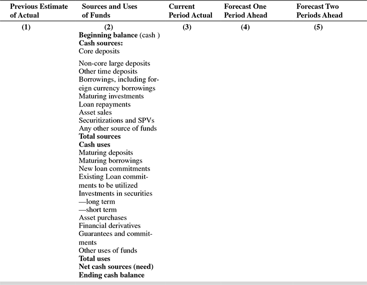
The ending cash balance could be a surplus or deficit at the end of the planning period.
What does the bank do in case of a surplus cash balance?
In case of a surplus, the bank has two options—(a) retain the surplus as cash; or (b) invest these funds in securities/loan assets. Though holding the surplus as cash would substantially reduce liquidity risk, the option would erode the bank’s profitability. Hence, the bank should be investing the surplus funds.
Here again, the bank has two alternatives. In the first alternative, the surplus can be invested in short-term assets, so that liquidity is not impaired, and yet the bank would be able to earn a small return on the funds invested. In the second alternative, the surplus can be invested in long-term assets, and the bank would borrow when the need for liquidity arises.
The bank’s decision would depend on whether it is an ‘asset-managed’ or a ‘liability-managed’ bank. An asset-managed bank would prefer to invest the surplus in low-yielding short-term assets, so that it can easily fund the liquidity deficits when they arise. A liability-managed bank would prefer to invest the surplus in high-yielding long-term assets and borrow to fund the liquidity deficit when it arises.
Illustration 12.11 will serve to clarify this.
ILLUSTRATION 12.11
Bank A wants to plan its liquidity, and has arrived at the cash inflows and outflows for the next 6 months as follows: (cash flows in ₹ crore).
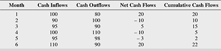
Assumption:
- All cash surpluses arise at the end of the relevant period.
- All cash deficits arise at the beginning of the relevant period.
- Additional information on expected yields on investments for different maturities is as follows:
| Period (in months) | Yield (% per annum) |
| 1 | 6% |
| 2 | 6.25% |
| 3 | 6.75% |
| 4 | 7.25% |
| 5 | 8% |
| 6 | 8.75% |
Case 1 The bank chooses to adopt asset management strategy.
It would, therefore, invest the surplus after meeting the deficit as follows:
- It would invest ₹10 crore for 2 months (months 2 and 3)
- It would invest ₹5 crore for 1 month (month 4)
- It would invest ₹2 crore for 2 months (months 5 and 6)
The bank’s total returns would amount to
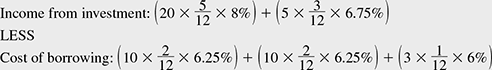
Case 2 The bank chooses to adopt liability management strategy
It would invest the surplus as and when it arises as follows:
- It would invest ₹20 crore for 5 months.
- It would invest ₹5 crore for 3 months.
It would also have to borrow to meet the deficits as follows:
- It will borrow ₹10 crore for 2 months.
- It will borrow ₹10 crore for 2 months.
- It will borrow ₹3 crore for 1 month.
The Bank’s net returns would amount to ₹0.53 crore, calculated as follows:
Interpretation of the Result The above comparison seems to show that the bank benefits more by liability management. However, in reality, the decision will depend on the following:
- The amount of time the surplus reserve position can sustain.
- The accuracy of yield forecasts.
It should also be noted that the cost of borrowing is assumed to be equal to the yield for the same period, a situation that may not be realistic in practice. Further, in a rising interest rate environment, the cost of borrowing may outpace the yield rate that has been locked in, thus, leading to refinancing risk for the bank.
Basel III—The International Framework for Liquidity Risk Measurements, Standards and Monitoring
In two documents published in December 2010 and January 2013 as part of the Basel III reforms described in earlier chapters, the Basel committee has presented reforms to strengthen liquidity risk management in banks. The latest documents build upon the Basel II framework for liquidity management as given in the ‘Principles for Sound liquidity risk management and Supervision’ (September 2008, accessed at www.bis.org) mentioned in an earlier paragraph.
The document published in December 2010, titled “Basel III: The International Framework for liquidity risk measurement, standards and monitoring”, (accessed at www.bis.org), the Committee mentions that the objective is to set rules and timelines to implement the liquidity portion of the Basel III framework (which we have described in the earlier chapter). The document published in January 2013, titled “Basel III: The Liquidity Coverage Ratio and liquidity risk monitoring tools” (accessed at www.bis.org), describes in detail the Liquidity Coverage Ratio (LCR) and its implementation timelines.
To recap from the earlier chapter, the LCR is a short term measure of the liquidity profile of banks and is measured as:
The Committee states that this ratio should be more than 100%. This implies that banks should hold High Quality Liquid Assets (HQLA) to more than compensate for liquidity outflows expected over a 30 day period. HQLA should comprise of unencumbered cash and assets that can be converted into cash with little or no loss of value to meet the liquidity needs of the bank over a 30 day period.
Specifically, the LCR will be introduced as planned on 1 January 2015, but the minimum requirement will begin at 60%, rising in equal annual steps of 10 percentage points to reach 100% on 1 January 2019. This graduated approach is designed to ensure that the LCR can be introduced without disruption to the orderly strengthening of banking systems or the ongoing financing of economic activity.
| 2015 | 2016 | 2017 | 2018 | 2019 | |
| Minimum LCR requirement | 60% | 70% | 80% | 90% | 100% |
A study of the components of the ratio as described in the document would show that the LCR builds on traditional liquidity coverage ratios and methodologies used internally by many banks (that have been outlined in earlier paragraphs of this section). However, the differences lie in the rigour of supervision by the regulator and the uniform definition for various classes of assets as well as cash inflows and outflows, taking into account off balance sheet items.
The summarized table given here (Basel III document of January 2013–Annexure IV) presents an illustrative list of the components of the numerator and denominator of the LCR.
The Numerator of the LCR – HQLA (The individual components of HQLA are to be multiplied by the factors given in the table)
The noteworthy feature of the above definition of HQLA is the recognition of the fact that all assets considered ‘liquid’ may not get converted to cash quickly without loss of value, due to their inherent risk and volatility factors. The Basel document contains detailed explanations of each of the above components.
The denominator of the LCR–net cash outflows over a 30 day period (The individual components of cash outflows and inflows are to be multiplied by the factors given in the table.)
It can be seen that the net cash outflows takes into consideration the possible cash outflows from off balance sheet commitments. Detailed definitions and explanations for each line item can be found in the Basel document of January 2013.
Some points to be noted are:
- It has been suggested that frequency of calculation and reporting of LCR by banks to supervisory authorities may be monthly or even more frequent. Under stressed situations, especially where the LCR falls below 100%, indicating that a bank does not have adequate liquidity to support its potential commitments, the supervisor should insist on immediate and more frequent reporting.
- The 2008 framework ‘Principles for sound liquidity risk management and supervision’ stipulates that a bank, at the consolidated level, should actively monitor and control liquidity risk exposures and funding needs at the level of individual legal entities, foreign branches and subsidiaries, taking into account the legal, regulatory and operational limitations to transfer of liquid funds within the group. This aspect continues to be relevant regardless of the scope of application of the LCR.
- For cross border banking groups, the LCR would be reported in the home currency. However, liquidity needs in each significant currency should also be calculated and reported. The rationale is clear. Banks and supervisors cannot assume that currencies will remain freely transferable and convertible in a stress period.
- In addition to the LCR, the document has identified metrics to enable consistent monitoring by banks themselves and their supervisors. These metrics, together with the LCR standard, is meant to enable supervisors assess the liquidity risk of a bank. Actions that supervisors can take in adverse situations are outlined in the Committee’s ‘sound principles’ document of 2008 (paragraphs 141–153, “Principles for sound liquidity risk management and supervision”, September 2008, accessed at www.bis.org).
- The metrics discussed in the January 2013 document include: (a) contractual maturity mismatch, (see Illustration 12.13 for a simple example); (b) concentration of funding; (c) available unencumbered assets; (d) LCR by significant currencies; and (e) market related monitoring tools. A detailed description of each of these metrics can be found in the January 2013 document. It can also be understood that the approaches outlined in the earlier paragraphs have been rigorously formalized in the Basel III framework for liquidity risk management.
The Group of Governors and Heads of Supervision (GHOS) is the oversight body of the Basel Committee on Banking Supervision (BCBS). The above proposals for regulating the short term liquidity of banks through the LCR is an outcome of its long standing deliberations on Basel III reforms and liquidity risk management. Following the successful agreement of the LCR, the Committee has launched the implementation of the Net Stable Funding Ratio (NSFR), which is a medium term measure of liquidity. This is a crucial component in the new framework, extending the scope of international agreement to the structure of banks’ debt liabilities.
To recap from the previous chapter:
NSFR will be a required standard from January 1, 2018, and the reporting will be not less than quarterly. The NSFR final standard was published by BCBS in October 2014. This document, titled Basel III: The net stable funding ratio can be accessed at http://www.bis.org/bcbs/publ/d295.pdf
The salient features of the calculation of available stable funding (ASF – the numerator of the ratio), and required stable funding (RSF- the denominator of the ratio) are given below.
- ASF
- The amount of available stable funding (ASF) is measured based on the broad characteristics of the relative stability of a bank’s funding sources.,
- These include the contractual maturity of the bank’s liabilities and the likelihood of different types of funding providers to withdraw their funding.
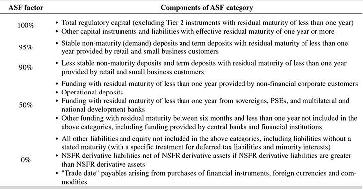
- The amount of ASF is calculated by first assigning the carrying value of an institution’s capital and liabilities to one of five categories as presented in Table 12.7
- The amount assigned to each category is then multiplied by an ASF factor, and the total ASF is the sum of the weighted amounts. The ASF factors, are pegged at various levels between 100% and 0%
- Carrying value represents the amount at which a liability or equity instrument is recorded before the application of any regulatory deductions, filters or other adjustments.
TABLE 12.7 LIABILITY CATEGORIES AND RELATED ASF FACTORSA SUMMARY
- RSF
- RSF relates to assets and off balance sheet exposures of banks
- The measure is based on the broad characteristics of the liquidity risk profile of the assets and off balance sheet exposures
- he amount of RSF is calculated by first assigning the carrying value of the bank’s assets to the categories listed
- The amount assigned to each category is then multiplied by its associated RSF factor as in Table 12.8. The RSF factors assigned to various types of assets indicate the approximate amount of funding that would be required to hold or roll over the asset. Assets are to be allocated to the appropriate RSF factor based on their residual maturity or liquidity value.
- The total RSF is the sum of the weighted amounts added to the amount of off balance sheet potential liquidity exposure, in turn multiplied by its associated RSF factor
TABLE 12.8 ASSET CATEGORIES AND RELATED RSF FACTORSA SUMMARY

The BCBS has also published extensive explanations to frequently asked questions on the NSFR in February 2017, which can be accessed at http://www.bis.org/bcbs/publ/d396.pdf
Annexure IV summarizes the key findings of a research conducted in May 2006 by the Bank for International Settlements42 and the lessons flowing from the financial crisis of 2007 manifested as principles for measurement and management of liquidity risk by the BIS.43
SECTION VI
APPLICABILITY TO BANKS IN INDIA
Interest Rate Derivatives in India
Indian participation in the derivative markets has accelerated only since the late 1990s. After the introduction of currency forwards in the 1980s, the Indian banking system saw no new instruments till 1997 when long-term foreign currency swaps began trading in the OTC markets.
Thereafter, the rise of derivatives in India has been swift—Interest rate swaps and FRAs were introduced as OTC products in July 1999, followed by several exchange-traded derivatives such as equity index futures (2000), equity index options (June 2001), stock options and stock futures later in the same year, and interest rate futures in June 2003.
In India, the different derivatives instruments are regulated by various regulators, such as Reserve Bank of India (RBI), Securities and Exchange Board of India (SEBI) and Forward Markets Commission (FMC). Broadly, RBI is empowered to regulate the interest rate derivatives, foreign currency derivatives and credit derivatives.
There are two distinct groups of derivative contracts:
- Over-the-counter (OTC) derivatives: Contracts are traded directly between two eligible parties, with or without the use of an intermediary and without going through an exchange. RBI is the primary regulator for OTC derivatives.
- Exchange-traded derivatives: Derivative products that are traded on an exchange.
Typically, participants in this market are broadly classified into two functional categories, namely, market-makers and users.
- User: A user participates in the derivatives market to manage an underlying risk.
- Market-maker: A market-maker provides bid and offer prices to users and other market-makers. A marketmaker need not have an underlying risk.
At least one party to a derivative transaction is required to be a market-maker. (It is to be noted that the definition is purely functional. For example, a market making entity, undertaking a derivative transaction to manage an underlying risk, would be acting in the role of a user.)
In India, all commercial banks (excluding Regional rural banks) and primary dealers can act as market makers. They are governed by the regulations in force. The users are typically business entities with identified underlying risk exposures.
At present, the following types of derivative instruments are permitted, subject to conditions and regulations in force:
- Rupee interest rate derivatives: Interest Rate Swap (IRS), Forward Rate Agreement (FRA), and Interest Rate Futures (IRF). IRS and FRA are OTC products, while Interest rate futures are exchange traded
- Foreign Currency derivatives: Foreign Currency Forward, Currency Swap and Currency Option – (Separate guidelines regarding Foreign Currency derivatives are issued by the regulator).
- Credit derivatives: Credit Default Swaps (CDS) on single name corporate bonds
OTC Derivatives in India Conventionally, OTC derivative contracts are classified based on the underlying into (a) foreign exchange contracts, (b) interest rate contracts, (c) credit linked contracts, (d) equity linked contracts, and (e) commodity linked contracts. The equity linked contracts and commodity contracts have been relatively insignificant and are absent in the domestic Indian OTC markets.
The structure of the OTC derivatives market (excluding equity and commodity linked derivatives) is broadly depicted in the chart below. (Instruments in bold face indicate that these are traded in the Indian market at present).
The Indian OTC derivatives market is dominated by Forex derivatives, followed by interest rates. In the OTC Forex derivatives, FX Swaps have been the most widely used instrument, followed by currency options and cross currency swaps. In the Indian markets, four OTC interest rate products are traded, viz., Overnight Index Swap based on overnight MIBOR (Mumbai Inter Bank Offered Rate - a polled rate derived from the overnight unsecured inter-bank market), contracts based on MIFOR (Mumbai Inter-Bank Forward Offered Rate—a polled rate derived from London Interbank Offer Rate (LIBOR) and USD-INR forward premium), contracts based on INBMK (Indian Benchmark Rate—a benchmark rate published by Reuters that represents yield for government securities for a designated maturity), and contracts based on MIOIS (Mumbai Interbank Overnight Index Swap—a polled rate derived from the MIBOR rates of designated maturity)

A typical characteristic of the Indian interest rate market is that unlike in the overseas inter-bank funds markets, there is very little activity in tenors beyond overnight and as such there is no credible interest rate in segments other than overnight. Absence of a liquid 3-month or 6-month funds market has been a hindrance for trading in Forward Rate Agreements (FRA), as also in swaps based on these benchmarks. This is reflected in trading volumes of the products as shown in Table 12.6. It is seen that the market for OTC interest rate derivatives is predominated by Interest Rate Swaps (IRS) with no activity in FRAs. It is also evident that MIBOR swaps dominate the market.
TABLE 12.6 TREND IN INTEREST RATE PRODUCTS TRADE

Another aspect of the market, which is not unique only to India, has been the concentration of market participants. Share of foreign banks is about 80 per cent of the total market volume with virtual absence of nationalized banks. Activity in the IRS market is fairly spread across the swap curve between 1-10 years. There are no swap trades beyond 10 years.
All scheduled commercial banks (SCBs) excluding Regional Rural Banks, primary dealers (PDs) and all-India financial institutions (please refer to Chapter 1 for a list of financial institutions) have been allowed to use IRS and FRA for their own balance sheet management as also for the purpose of market making. The non-financial corporations have been allowed to use IRS and FRA to hedge their balance sheet exposures, with a caveat that at least one of the parties in any IRS/FRA transaction should be a RBI regulated entity. In addition to the RBI circular of 1999 (dated July 7,1999) which lays down principles for accounting and risk management for positions in IRS/FRA, RBI has, in 2007 (RBI circular dated April 20, 2007), released comprehensive guidelines on derivatives comprising general principles for derivatives trading, management of risk and sound corporate governance requirements along with a code of conduct for market makers.
Interest rate options were introduced in December 2016.
The guidelines for interest rate options and periodical updates in the guidelines can be accessed at www.rbi.org.in
Reporting of OTC derivatives–CCP and TR
(Sources: RBI, May 2011, Report of the Working group on reporting of OTC interest rate and forex derivatives, and RBI, 2012, Report of the Working Group on enhancing liquidity in the Government securities and Interest rate derivatives markets)
The OTC derivatives market is characterized by large exposures between a limited number of market players. When the market is characterized by the existence of a few market makers, most of the activity takes place between these players and disruptions at any major dealer would soon transmit to other financial institutions and spread contagion to the entire market. The risk in the OTC derivative market also emanates from the opacity in the market that constrains the market participants from assessing the quantum of risk held with the counterparty. Further, with increase in volumes and complexities of the OTC derivatives, the non-standardized infrastructure for clearing and settlement also becomes a major impediment in containing risk, especially in the wake of the financial crisis of 2007-08. At the G 20 Toronto summit declaration of June 2010, Central banks and Market regulators agreed to initiate measures to enhance the post trading infrastructure in the OTC derivative markets.
Establishing Central counterparties (CCP) and Trade Repositories (TR) were two of the important commitments made at the above Summit.
A CCP is a financial institution that interposes as an intermediary between security (including derivatives) market participants. This reduces the amount of counterparty risk that market participants are exposed to. A sale is contracted between the seller of a security and the central counter party on one hand and the central counterparty and the buyer on the other. This means that no market participant has a direct exposure to another and if one party defaults, the central counterparty absorbs the loss. Settlement through a central counterparty has been progressively used on most major stock and security exchanges. However, a CCP based system can lead to concentration of risk with the CCP, which issue needed to be addressed.
On the other hand, the objective of TRs is simply to maintain an authoritative electronic database of all open OTC derivative transactions. It collects data derived from centrally or bilaterally clearable transactions as inputted/verified by both parties to a trade. An important attribute of a TR is its ability to interconnect with multiple market participants in support of risk reduction, operational efficiency and cost saving benefits to individual participants and to the market as a whole. The typical drawback of the OTC market is that the information concerning any contract is usually available only to the contracting parties. While expanding the scope of availability of information, it became pertinent to distinguish between information available to regulators, to market participants and to public at large. Post trade processing services is another important function of TR.
The reporting arrangement in interest rate derivatives in India follows a two tier system. Since at least one party to an OTC interest rate derivatives transaction is a RBI regulated entity, there has been an elaborate prudential reporting requirement in so far as the risk implication of the derivative positions for the entity is concerned.
In 2003, an internal Working Group of the RBI on Rupee derivatives had recommended a centralized clearing system for OTC derivatives through Clearing Corporation of India Ltd (CCIL). Preparatory to introduction of centralized clearing as also to get a better understanding of interest rate derivative market in India, RBI, in 2007, made it mandatory for the RBI regulated entities to report inter-bank/PD transactions in interest rate derivatives (FRAs and IRS) on a platform developed by the CCIL. Subsequently, all inter-bank/PD deals were required to be reported by the banks and PDs on the CCIL platform within 30 minutes of initiating the transaction. The information captured through this reporting system is comprehensive. Further, CCIL’s evolution as a repository owed to a regulatory mandate, unlike repositories like DTCC which evolved out of a need to facilitate post trade processing.
As noted above, In India, RBI initiated measures for transaction-wise reporting of IRS Trades and mandated reporting of all inter-bank trades to Clearing Corporation of India Limited (CCIL) in August 2007. It is noteworthy that the Indian financial market has had a well-functioning CCP, viz., CCIL that has been offering CCP-guaranteed settlement for transactions in government securities, a few money market instruments, and forex i.e., dollar-rupee transactions. However, CCIL does not provide post trade services except aggregate data dissemination.
From April 2014, all entities regulated by the Reserve Bank should report their secondary market OTC trades in Corporate Bonds and Securitized Debt Instruments within 15 minutes of the trade on any of the stock exchanges (NSE, BSE and MCX-SX). These trades may be cleared and settled through any of the clearing corporations (NSCCL, ICCL and MCX-SX CCL). (RBI circular dated February 24, 2014)
The Need for TR (Trade Repositories)
TRs help in obtaining a clear understanding of:
- the size and liquidity of the market.
- the scale of participation by various entities.
- the size and risk profile of outstanding positions and their potential impact in the event of a default.
- the evolution of price in the market which promotes transparency.
They also help in the development of tools that allow regulators and other stake holders to have access to more information and thereby identify emerging systemic risks.
Currently the major TRs globally are: (in order of their establishment)
- CDS Trade Repository – DTCC & Markit (discussed in the chapters on ‘Credit Risk’)
- IRS Trade Repository – TriOptima
- REGIS-TR (promoted jointly by Clearstream and Bolsas y Mercados Espanoles
- Equity Trade Repository – DTCC & Markit (since 2005, expanded to provide matching services for interest rate swaps and swaptions, equity swaps and variance swaps)
- Credit Derivatives – DTCC Europe
- All asset classes – Xtrakter owned by Euroclear
While DTCC contributes its Deriv/SERV matching and confirmation engine, Markit’s data and valuation provides the much needed post trade valuation services. This alliance provides a fully integrated system for processing OTC derivatives across borders and asset classes to provide a service that helps a wide range of market participants achieve greater certainty in their transaction processing. It also addresses the challenges of rapid growth, increased cost and operational risks associated with the OTC derivative markets.
TriOptima, a Stockholm-based technology company was selected by ISDA to operate as an interest rate derivatives TR. A number of broker-dealers, buy-side firms and industry associations, committed to record all interest rate derivatives trades in this TR. The OTC Derivatives Interest Rate Trade Reporting Repository (IR TRR) launched by TriOptima in early 2010 was an important step towards improving transparency in the global OTC derivatives markets.
An important innovation in OTC derivative markets introduced during the last few years relates to portfolio compression services offered by TriOptima. Since the only way to exit a position in an OTC derivative is to enter into another with opposite pay off, the gross notional outstanding multiplies manifold as a result. Apart from the fact that this does not capture the economic essence of the portfolios, it increases the demand on capital for the regulated entities. TriOptima’s TriReduce and TriResolve services reportedly offer multilateral netting with bilateral settlement whereby an entity can extinguish its OTC derivative positions without affecting its MTM value or the PV01(change in price of a bond for a change in yield in absolute monetary value rather than percentage as in modified duration. PV01 is measured as the product of the modified duration and price/value. For more on modified duration please refer to the Annexure to this chapter).
In India too, the service has been used by the IRS portfolio holders with significant reduction in the gross notional positions. The first such exercise was undertaken in July, 2011 wherein a compression of 94.30 per cent of the submitted trades was achieved. The second cycle of compression was carried out in March 2012 with a compression of 90.31 per cent. As already stated, ‘Portfolio compression’ reduces the overall notional size and number of outstanding derivatives contracts in the portfolio without changing the overall risk profile of the portfolio. During this period, RBI has also taken initiatives to strengthen the legal framework in respect of OTC derivatives in interest rates and forex.
The Exchange Traded Interest Rate Derivatives in India
Interest rate futures (IRF) were introduced in June 2003 when National Stock Exchange (NSE) launched three IRF contracts - futures on 10-year notional G-Sec with a coupon of 6 per cent, 10-year notional zero-coupon G-Sec and 91-Day T-Bills. However, these contracts did not attract enough market interest since its introduction and soon became defunct. The use of ZCYC to determine the daily settlement price and for MTM of the contract resulted in large basis risk for participants trying to hedge their cash market positions through the futures market thereby making the futures contract unattractive, if not risky (All the terms – ZCYC, MTM and basis risk – have been described in earlier chapters). Further, the prohibition of banks from taking trading positions in the futures market had resulted in very low/negligible liquidity in this market.
A second joint committee of the RBI and Securities and Exchange Board of India (SEBI) based its recommendations on the above findings in June 2009. Its primary suggestion was to introduce physically settled Interest rate futures contract on 10 year Government of India (GoI) coupon bearing security.
Subsequently, RBI issued Interest Rate Futures (Reserve Bank) Directions, 2009, on August 28, 2009, and followed it up with amendments upto December 2011. The latest Directions have come into effect in December 2013. The RBI has included cash settlement for 10 year Government of India (GoI) securities, which can also be settled by physical delivery. The other underlying securities included are 91 day Treasury bills, 2 year, 5 year and coupon bearing GoI securities, which are eligible for cash settlement.
Banks are permitted to participate in IRF both for the purpose of hedging the risk in the underlying investment portfolio and also to take trading position. However, banks are not allowed to undertake transactions in IRFs on behalf of clients. Similarly, stand-alone Primary Dealers are allowed to deal in IRF for both hedging and trading on own account and not on client’s account.
However, experts attribute lack of activity in IRF to structural factors such as lack of liquidity in the underlying cash market, SLR prescriptions and HTM facility. Other factors normally cited for the lack of market activity are (a) banks and MFs have portfolio duration of less than 5 years; (b) IRF contract cannot be used as a perfect hedge; (c) the market hesitancy to take a view on long-term interest rates; and (d) lack of significant buy side interest in a rising interest rate cycle and over supply of G-secs.
The latest guidelines on exchange traded derivatives can be accessed at www.rbi.org.in
ALM Framework for Indian Banks
From 1 April 1999, banks in India were expected to implement an effective ALM system, the guidelines for which were contained in RBI circular dated 10 February 1999. The salient features of this system are as follows:
- Banks were expected to form an ALCO headed by the bank’s chief executive.
- The ALM process rested on three pillars—ALM information system, ALM organization and the ALM process
- The ALM information system emphasized the need for accurate and timely information to assess risks of individual banks.
- The prerequisite for an effective ALM organization is strong commitment from the bank’s senior and top management. The ALCO of the bank would be responsible for ensuring proper asset liability management as set by the bank’s Board of directors.
- Though the scope of the ALM process would encompass management of liquidity risk, market risk, trading risk, funding and capital planning and profit planning, the RBI guidelines primarily address liquidity and interest rate risks.
Liquidity Risk Management Guidelines Primarily, liquidity was to be tracked through maturity or cash flow mismatches. For this purpose, a standard tool was to be adopted, involving the use of a maturity ladder and calculation of cumulative surplus or deficit of funds at selected maturity dates. Within each specified time bucket, there could be mismatches between expected cash inflows and outflows. The main area of concern here would be the short-term mismatches—those up to 28 days. Hence, RBI had asked banks to keep the mismatches (negative gap) during this time period within 20 per cent of cash outflows in each time bucket. Bank assets and liabilities are grouped into different maturity profiles and presented in the statement of structural liquidity for decision making.
The statement of structural liquidity would essentially show all expected cash inflows and outflows during the specified period. A maturing liability will be a cash outflow while a maturing asset would represent a cash inflow. In determining the likely timing and magnitude of these cash flows, banks will have to make several assumptions based on whether they resort to asset management or liability management.
The guidelines also suggest a format that would enable banks to estimate short-term dynamic liquidity, i.e., monitor their short-term (1 to 90 days) liquidity, as in the cash flow method described in Section V.
Interest Rate Risk Management Guidelines44 RBI has proposed in April 2006 that the Modified Duration Gap approach be adopted for interest rate risk management. The steps to be followed for computing the Modified DGAP would be as follows:
- Identify variables such as principal amount, maturity date/re-pricing date, coupon rate, yield, frequency and basis of interest calculation for each item/category of asset/liability (including off-balance sheet items).
- Generate the bucket-wise (additional time buckets have been proposed for longer lending horizons) cash flows for each item/category of asset/liability/off-balance sheet item.
- Determine the yield curve for arriving at the yields based on current market yields / current replacement cost for each item/category of asset/liability/off-balance sheet item.
- Assume the mid-point of each time bucket as representing the maturity of all assets and liabilities in that time bucket.
- Calculate the Modified Duration of each category of asset/liability/off-balance sheet item using the variables in (1).
- Determine the weighted average Modified Duration of all the assets (DA) and similarly for all the liabilities (DL), including off-balance sheet items.
- Derive the Modified Duration Gap as;
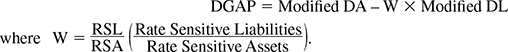
DA = Weighted average Modified Duration of assets and
DL = Weighted average Modified Duration of liabilities.
- Calculate the Modified Duration of Equity as = DGAP × Leverage, where Leverage = RSA / Equity. In this case, ‘equity’ will represent capital funds. It is proposed that banks report monthly to RBI the interest rate sensitivity as evidenced by the modified duration approach.
Illustration, 12.12 excerpted from the RBI guidelines, will serve to clarify the mechanics, which can be applied to assets, liabilities and equity:
ILLUSTRATION 12.12
| EVE | (₹ in Crores Amount |
|---|---|
| Net worth | 1,350.00 |
| RSA | 18,251.00 |
| RSL | 18,590.00 |
| Modified duration of gap | |
| DA (Weighted modified duration of assets) | 1.96 |
| DL (Weighted modified duration of liabilities) | 1.25 |
| Weight = RSL/RSA | 1.02 |
| DGAP = DA – W × DL | 0.69 |
| Leverage ratio = RSA / (Tier 1 + Tier 2) | 13.52 |
| Modified duration of equity = DGAP × Leverage Ratio | 9.34 |
| For a 200 bp | 18.68% (9.34 × 2) |
| Rate shock the drop in equity value is |
The basic slotting of various assets and liabilities based on their maturity profile and interest rate sensitivity is shown in Annexure V. It is to be noted that these profiles are fine-tuned in subsequent RBI guidelines to refine the process of interest rate risk and liquidity risk management.
Liquidity Risk Management in Indian Banks
The global financial crisis of 2007 has highlighted, like never before, the role of prudent liquidity management as the cornerstone of financial stability. On November 7, 2012, RBI released guidelines for liquidity risk management, based on the documents Principles for Sound Liquidity Risk Management and Supervision as well as Basel III: International Framework for Liquidity Risk Measurement, Standards and Monitoring published by the Basel Committee on Banking Supervision (BCBS) in September 2008 and December 2010 respectively. Banks had to implement the guidelines immediately. However, these guidelines have been further refined based on the January 2013 document of the Basel committee titled ‘Basel III: The Liquidity Coverage Ratio and Liquidity Risk Monitoring Tools’, the salient features of which were discussed in Section V.
The RBI circular on LCR was issued in June 2014 and can be accessed at https://rbidocs.rbi.org.in/rdocs/notification/PDFs/CA09062014F.pdf. The measurement process shown in Section V has been customized to suit local practices. The LCR requirement would be binding on banks from January 2015. In order to provide a transition time for banks, the requirement would be minimum 60% for the calendar year 2015 i.e. with effect from January 1, 2015, and rise in equal steps to reach the minimum required level of 100% on January 1, 2019.
RBI issued draft guidelines for implementing NSFR standards in March 2015. This document can be accessed at www.rbi.org.in.
As we have seen earlier, a ‘negative gap’ within a time bucket indicates that maturing assets during that time period are lower than the liabilities maturing during the same period. This implies that the cash flows from assets (say interest payments, principal repayments, etc., from loans, advances or investments) would not be sufficient to cover the demands made by depositors and other creditors during the period under consideration.
The simple Illustration 12.13 shows the impact of ‘negative gap’ on liquidity management through simple matching of ‘maturities’. The illustration is an example of “contractual maturity mismatch” as a liquidity monitoring tool, as mentioned in both the Basel document of 2013 and RBI guidelines of June 2014
ILLUSTRATION 12.13 MATURITY GAP MATCHING—A SIMPLE EXAMPLE
Bank D has the following assets and liabilities classified by maturity.45 Note that these are maturing liabilities and assets in each time bucket.
| Maturity Mths | Liabilities | Assets |
|---|---|---|
| Less than 1 | 7 | 10 |
| 1–3 | 13 | 8 |
| 4–6 | 11 | 10 |
| 7–12 | 9 | 20 |
| 13–24 | 24 | 27 |
| 25–36 | 29 | 19 |
| Above 36 | 10 | 9 |
We will now find the GAP in each time bucket, affix a sign to this GAP, and then find the cumulative gap.
Matching assets and liability by maturity
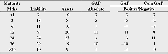
What can we conclude about the bank’s liquidity risk from the above table?
We see that in the near term, i.e., up to 6 months, the bank has two time buckets of negative gaps, which are not offset by the positive gap in the first time band, up to 1 month.
This implies that the bank is subject to liquidity risk even if all the assets yield cash flows as expected during this period. Further, if there is a shortfall in expected cash flows from maturing assets or if there is unexpected increase in demand from liability holders, the bank’s liquidity position will deteriorate. Hence, the bank has to plan ahead for alternative sources of liquidity over the next 6 months.
This approach not only limits liquidity risk exposure in specific time buckets, but also recognizes the cumulative impact on liquidity over time periods in the near future, which is the most relevant for banks’ liquidity.
According to these guidelines, banks have to undertake dynamic liquidity management. The guidance for slotting future cash flows is shown in Annexure V.
CHAPTER SUMMARY
- Prior to the 1970s, many firms in the developed countries intentionally mismatched their balance sheets, and borrowed short and lent long to earn a spread. Things started to change in the 1970s, which ushered in a period of volatile interest rates that continued into the early 1980s. The 1980s and 1990s also saw a new wave of banking crises that arose more from sharp movements in asset prices or sharp contractions in market liquidity or credit risk concentrations, defying the traditional regulatory prescriptions of deposit insurance or lender of last resort advances. The global financial crisis of 2007 has highlighted the need for policy makers and regulators to seek new preventive measures to handle banking risks.
- Risk management is uniquely important for financial institutions because, in contrast to firms in other industries, their liabilities are a source of wealth creation for their shareholders. Asset-liability risk is a ‘leveraged’ risk since the capital base of banks is small relative to its assets or liabilities. Hence, small percentage changes in assets or liabilities can translate into large percentage changes in capital.
- ALM is concerned with strategic balance sheet management. Risks caused by changes in interest rates and exchange rates, credit risk and the bank’s liquidity position have to be monitored and mitigated. Techniques of ALM have been evolving over time.
- Banks typically have an ALCO, that comprises of a group of top or senior management personnel entrusted with the responsibility of managing the bank’s assets and liabilities to balance the various risk exposures, to enable the bank achieve its operating objectives.
- Interest rate risk is the exposure of a bank’s financial condition to adverse movements in interest rates. If accepted and managed as a normal part of banking business, interest rate risk can be used to enhance profitability and shareholder value. However, excessive interest rate risk could lead to substantial volatility in earnings and, thus, affect the underlying value of the bank’s assets, liabilities and off-balance sheet instruments.
- The two most common perspectives for assessing a bank’s interest rate risk exposure are (a) the earnings perspective that focuses on short-term earnings, and (b) the economic value perspective that looks at the long-term economic viability of the bank.
- Interest rate risk arises from several factors fundamental to the business of banking. Some of the most discussed sources of interest rate risk are: Repricing risk, Yield curve risk, Basis risk and Embedded optionality.
- Banks use various techniques to measure the exposure of earnings and economic value to changes in interest rates. These techniques range from simple calculations relying on basic maturity and repricing tables based on current and projected on- and off-balance sheet positions, to highly sophisticated dynamic modelling techniques. Some of the popular approaches include: Gap analysis, EAR models and EVE models, as well as DGAP analysis models used to immunize the MVE.
- A popular alternative to mitigate the interest rate risk on its investments is the use of Interest Rate Derivatives (IRDs). Banks use IRDs to transform some fixed-rate investments into floating-rate assets. They also use IRDs to transform floating-rate liabilities into fixed-rate liabilities. IRDs are simply contracts used to hedge other positions that expose them to risk, or speculate on anticipated price moves. In most cases, banks use IRDs to replicate balance sheet transactions with off-balance sheet contracts, so that contingent positions are created.
- Some of the most basic and widely used IRD contracts are—Swaps, Futures, FRAs, Options, Caps/Floors/Collars and ‘Swaptions’.
- Basel committee has published extensive guidelines in April 2016 to enable measuring and managing interest rate risk in the Banking Book
- Liquidity risk is the risk that the bank may not be able to fund increases in assets or meet liability obligations as they fall due without incurring unacceptable losses. Of the four specific forms of risk that impact banking operation—credit risk, market risk, operational risk and liquidity risk—the first three have been extensively studied and commonly incorporated into existing capital allocation frameworks. However, at present, there is no technique for modelling liquidity risk that has wide acceptance. Basel III has introduced LCR in January 2013 for regulating liquidity. The guidelines for NSFR were published in October 2014.
- The alternative approaches prevalently used by banks for Liquidity Risk Management are (a) Asset Management, and (b) Liability Management.
- Some of the forward-looking tools for Liquidity Risk Management prevalently used include: (a) Projected sources and uses of funds over the planning horizon, (b) the working funds approach, (c) cash flow or funding gap report, (d) funding concentration analysis, (e) funds availability report and so on. A few typical retrospective tools include ratio analysis and historical funds flow analysis.
- Indian participation in the derivative markets has accelerated only since the late 1990s. A lion’s share of banks’ off-balance sheet exposures is attributable to derivatives activity. In December 2013, the RBI directives on interest rate futures has attempted to address some shortcomings of the earlier guidelines on interest rate derivatives. RBI permitted Interest rate options since December 2016.
- From 1 April 1999, banks in India were expected to implement an effective ALM system. The ALCO of the bank would be responsible for ensuring proper asset liability management as set by the bank’s Board of directors.
- Though the scope of the ALM process would encompass management of liquidity risk, market risk, trading risk, funding and capital planning and profit planning, the RBI guidelines primarily address liquidity and interest rate risks.
TEST YOUR UNDERSTANDING
- Rapid fire questions
Answer ‘True’ or ‘False”- Banking operations are subject to various independent risks
- Risk management means reduction of risk
- Asset liability risk arises due to mismatch between assets and liabilities
- ALM is strategic balance sheet management
- Modern ALM focusses more on earnings and value creation rather than just short term earnings
- ALCO also manages credit risks
- Interest rate risk is the exposure of a bank’s financial condition to adverse movements in interest rates
- Interest rate risk affects only the bank’s earnings
- Interest rate risk affects the bank’s off balance sheet instruments
- Optionality is a source of interest rate risk
Check your score in Rapid fire questions
- False
- False
- True
- True
- True
- False
- True
- False
- True
- True
- Fill in the blanks with appropriate words and expressions
- The ————— perspective for assessing a bank’s interest rate risk exposure focuses on short term earnings
- The ————— perspective for assessing a bank’s interest rate risk exposure focuses on the long term viability
- The net interest income is the difference between ————— from ————— and ————— on —————
- The static GAP is the difference between ————— and ————— in each time bucket
- When risk sensitive assets are more than risk sensitive liabilities across a time interval in static GAP analysis, the bank is termed ————— sensitive
- The DGAP measure is ————— adjusted
- The contract where two parties agree to exchange periodic payments is called a ————— contract
- Expand the following abbreviations in the context of the Indian financial system
- Test your concepts and application
- Why is refinancing risk an important interest rate risk?
- How does a rise or fall in interest rates affect the market value of both assets and liabilities?
- Which is the predominant risk in the following transactions carried out by a bank?
- It finances a 5-year fixed rate loan with a 1 year certificate of deposit
- A British bank uses deposits in GBP to lend in the euro market for fixed rates
- What is the importance of ‘maturity buckets’ in the GAP models? Why is the length of time selected for repricing assets and liabilities important when using the models?
- Calculate the Maturity GAP and the impact on NII for: (a) an increase in interest rates of 100 bps, and (b) decrease in interest rates of 100 bps, in each of the following positions:
- Rate sensitive assets ₹200 crore, rate sensitive liabilities ₹100 crore
- Rate sensitive assets ₹100 crore; rate sensitive liabilities ₹150 crore
- Rate sensitive assets ₹150 crore; rate sensitive liabilities ₹140 crore
What conclusions can you draw from the above results?
- A bank’s ALCO is reasonably certain that interest rates are going to rise over the next 6 months. How should it adjust the bank’s Maturity GAP to take advantage of this increase? Would the GAP be maintained differently if interest rates were expected to fall? How easy is it in practice to carry out adjustments in GAP?
- In the above case, if the bank were using the Duration GAP, would the decision be any different? Substantiate your answer.
- A Bank has the following assets and liabilities on its balance sheet—it has loans of ₹10,000 crore and no other assets; it has deposits of ₹8,500 crore and a capital of ₹1,500 crore. Assume that the average maturity of the loan is 4 years, and the average maturity of the deposits is 2 years. Also assume that the loan and deposit are at book value, and are repayable only at the end of the maturity period.
- If the interest rate on both the loan and deposit is at 9 per cent, what is the MVE?
- If the MVE is to be made zero in the above case, what should be the average maturity of the deposits?
- If MVE is to be zero, what should be the average interest rate on deposits that the bank should offer?
- A bank’s balance sheet has the following assets: cash of ₹50 crore and other assets of ₹150 crore. The corresponding liabilities are deposits of ₹140 crore, borrowings of ₹30 crore, and other liabilities of ₹30 crore. One of the bank’s valued customers wants the sanctioned credit limit of ₹12 crore to be disbursed immediately. How will the bank’s balance sheet look if (a) the bank adopts asset management and (b) the bank adopts liability management, in complying with the customer’s request.
- At March end, 2006, Bank X showed the following position:
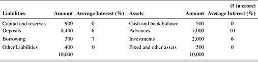
- Calculate the rate sensitive gap, assuming that all interest bearing assets and liabilities are rate sensitive.
- If the interest rates were to move as follows over the next 1 year, what would the GAP be?
Deposits 6.75% Borrowings 8.00% Advances 11.00% Investments 6.80% - If the average duration of assets were 4 years, and the average duration of liabilities were 3 years, and the current interest rate were at 10 per cent, what would be the change in the market value of the equity due to increase in interest rate by 100 bps?
- How can Bank X immunize the MVE?
- Bank Y’s ALCO expects the interest rates to move as follows:
Change in Interest Rates Probability –0.5% 0.10 +0.5% 0.20 –1.0% 0.30 +1.0% 0.40 If the earning assets of the bank are at ₹50,000 crore, NII is ₹1,500 crore, and the bank expects a variation of 10 per cent in NII,
- what is the Target GAP for each of the possible changes in interest rates?
- what will be the change in NII be for different levels of GAP?
- If RSA and RSL are decreased by the same amount, which of the following will be true?
- Gap remains unchanged, gap ratio increases
- Gap remains unchanged, gap ratio decreases
- Gap and Gap ratio both remain unchanged
- Gap and Gap ratio will change
- None of the above is applicable
- Bank B has the following position of assets and liabilities: ₹10 crore in short-term government securities, ₹6 crore line of credit to borrow in the short term and repo market, and ₹3 crore excess cash reserve with the central bank. It has also borrowed ₹5 crore in the call money market to meet urgent requirements.
- What are the bank’s total available sources of liquidity?
- What are the bank’s total uses of liquidity?
- What conclusions do you draw from the net liquidity position of the bank?
- How sensitive will a bank’s MVE be to a change in interest rates under each of the following scenarios? Consider the effects of rising and falling interest rate environments.
- Seventy per cent of the bank’s assets are in 15 year housing loans and infrastructure loans
- The bank is paying less than market rates on a major portion of its term deposits, and market interest rates move upwards
- Eighty per cent of the bank’s investment portfolio is in short-term investments, due to mature in the next two quarters
- Bank Z is liability sensitive. The management seeks protection from interest rate risk. Which of the following would be a better hedge—interest rate cap, floor, collar or reverse collar? Would the management take a different stand if the bank were asset sensitive?
TOPICS FOR FURTHER DISCUSSION
- Study the financial statements of some large banks in the country. What are the risks they carry on their balance sheets, and in their off-balance sheet transactions? Can you quantify the risk?
- All banks in India mandatorily show the maturity profile of liabilities and assets on their financial statements. Analyze the maturity profiles. Can you arrive at conclusions regarding the interest rate and liquidity risks these banks carry?
- Study the derivative transactions entered into by major banks. What are the risks involved? How serious are these risks for the banks?
- Calculate LCR of major banks using Basel III guidelines of January 2013.
SELECT REFERENCES
- Chacko, George, and Sjoman, Anders, 2006, ‘Introduction to Interest rate options’, Harvard Business School Publishing.
- FDIC, 2005, ‘Risk Management Manual of Examination Policies’, Section 3.8, ‘Off balance sheet activities’ accessed at [email protected]
- Federal Reserve Bank of Kansas City and Federal Reserve Bank of St Louis, ‘Insights for Bank Directors’, The Federal Reserve Center for online learning.
- Harvard Business School, 1995, ‘Interest Rate Derivatives’.
- Hong Kong Monetary Authority, 2004, Supervisory Policy Manual, ‘Liquidity Risk Management’.
ANNEXURE I
THEORIES OF INTEREST RATES
Interest rate risk management can be effective only if interest rate forecasts are realistic and accurate. The forecasts are primarily based on the shape of the future yield curve.
The yield curve, simply stated, is a measure of the market expectations of movements in future interest rates, given the current market conditions. It is shown as a graph comparing yields on securities of different maturities, assuming other factors such as, default risk or marketability as identical for all the securities being compared. This is also known as the ‘term structure’ of interest rates.
Government securities are considered risk free and their yields are often used as the benchmark for other instruments with similar maturities. The yield curve is constructed as a graph in which the ‘yield to maturity’ is plotted on the vertical axis and the number of years to maturity on the horizontal axis. The two essential assumptions made while graphing are that the securities are noncallable and are akin to zero coupon bonds that mature on the common payment date. Typically, yield curves for risky bonds will be at a higher level on the graph than the yield curves for comparatively safe bonds.
The exact shape of the yield curve is closely scrutinized since it can be different at any point in time. An upward sloping yield curve is typical of economic recovery, where the long-term interest rates are expected to exceed the short-term interest rates and the spot rates are increasing. Similarly, when the yield curve tends to slope downward, indicating that long-term interest rates are less than short-term rates and the spot rates are declining, the economy could be heading for a recession. Hence, a change in the shape of the yield curve serves as a signal to the investors to change their outlook on the economy.
The slope of the yield curve is also seen as an important indicator—the greater the slope, the greater is the gap between short- and long-term interest rates.
In order to further elaborate, there are essentially three patterns created by the yield curves, which are as follows:
- Normal Yield Curve This is the yield curve shape that is expected to form during normal market conditions, in which investors typically believe that the economy will grow at a reasonable rate in line with expectations and there will be no sudden or significant changes in critical indicators such as inflation rates. The yield curve will be generally upward sloping and the market expects longer-term fixed income securities to offer higher yields than short-term fixed income securities, due to the risks associated with time. With increase in the difference between short- and long-term yields, the curve becomes ‘steep’.
 Source: investopedia.com
 - Flat (or Humped) Yield Curve This type of yield curve sends out varying signals, making it difficult for the market to determine the direction of interest rate movements in future. A flat yield curve usually occurs when the market is in a transition phase. Here, the shorter- and longer-term yields are very close to each other. When the yield curve is flat, the investors would prefer to invest in fixed income securities with the least risk or the highest credit quality. Under circumstances leading to a decline in the long-term interest rates, a flat curve can sometimes lead to an inverted curve.
 Source: investopedia.com
 - Inverted Yield Curve These yield curves, though rare, indicate abnormal market conditions where the expectations of investors are entirely in contrast with thoset demonstrated by the normal yield curve. The inverted yield curve signals that long-term bonds may yield less than short-term securities. This phenomenon happening in a growing economy could indicate upcoming recession.
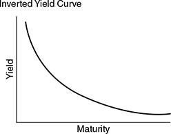 Source: investopedia.com
The Theories Behind Yield Curve Shapes
The shape of the yield curve is explained through a few popular theories. Before we describe the theories, we will have to understand the two terms – ‘spot’ rate and ‘forward’ rate.
The spot rate is the prevailing interest rate that can be obtained from the following equation:
[1 + spot interest rate for a maturity t years [St]]
The forward rate is the interest rate that is expected to prevail at some future specified dates. According to a popular theory (Pure Expectations Theory), the current forward rate is an unbiased predictor of future spot rates. In other words, a bank would earn identical yields on a two-year loan, irrespective of whether the loan tenure is of two years or one year, rolled over at the end of the first year. Such a rate, at which the rolled over loan would earn an identical yield is called the ‘implicit forward interest rate’. Thus, the implicit forward interest rate would, in effect, represent the future rate of a short-term loan when rolled over and would be equal to the present long-term rate. In mathematical terms, the equation can be generalized as follows:
where rt = yield on a loan with maturity ‘t’
rt−1 = yield on loan with maturity ‘t − 1’
Ft−1 = implicit forward interest rate
We will now provide a brief overview of some of the popular theories.
Pure Expectations Theory This theory is also called the ‘unbiased expectations theory’ and the assumption here is that forward rates are unbiased estimates of expected spot rates. In other words, the theory attempts to explain the difference in yields on securities with different maturities arising due to varying investor expectations regarding interest rate movements in future. This implies that the investors will prefer securities with the highest return, regardless of the maturities. For example, an investor with a three-year planning horizon may choose one of the following alternatives to achieve his investment objective: (a) he can invest in a security with a maturity period of three years or (b) invest for one year and roll over twice or (c) invest for two years and roll over for one year or (d) invest for one year and roll over for two years thereafter. According to this theory, the interest rate that equates the return on a series of short-term securities with the return on a long-term security carrying the same final maturity would represent the market’s expectation of the future interest rate. An inherent assumption is of course that the alternatives enumerated above can be carried through without cost. Therefore, after summarizing, the theory hypothesises that (a) the long-term interest rates are an average of the current and expected future short-term interest rates, (b) the expected short-term interest rate is the market forecast of future interest rates and (c) the investors would substitute maturities for better yields. Going by this theory, an upward sloping yield curve augurs an increase in interest rates, while a downward sloping yield curve is a signal that interest rates would dip in future. However, the interpretation could be too simplistic since an upward sloping curve can shift downwards in its entirety when rates decline, yet preserving the upward slope.
Liquidity Theory This theory is also called the ‘liquidity premium theory’ and is an extension of the pure expectations theory. The liquidity theory incorporates the additional factor of the investor’s expectations of ‘price risk’ in forecasting the market rates. Even if expected returns are identical for long-term securities and a series of same maturity shortterm securities, the investors would have to be induced into buying long-term securities due to the price fluctuations that could arise over a fairly longer term. That is, if an investor receives a return of 10 percent for securities with maturities of both one and two years’ maturities, he may prefer to have the option of investing for a year and roll over for another, if interest rates are still favourable after a year. In other words, investors would expect additional return for investing in long-term securities in the form of a risk premium. Essentially, therefore, long-term rates would be set as the average of current and expected short-term rates plus a ‘liquidity premium’. In effect, the forward rate, too, would then equal the expected rate plus a liquidity premium. The yield curve is theoretically expected to be upward sloping since the long-term rates are always expected to stay above the short-term rates and the imposition of a liquidity premium exerts an upward bias. However, in the very long term, the yield curve implicit forward interest rate would tend to flatten out, since there is a little differential price risk at longer maturities. Further, if the yield curve becomes inverted, there would be expectation of a very sharp drop in the short-term rates to compensate for the heightened liquidity premiums.
Preferred Habitat Theory While not contesting the validity of the liquidity premium, this theory argues that it cannot be extended to cover all maturities. The maturity preference of borrowers and lenders depends on their unique needs, preferences and constraints. Hence, the presence of a premium might induce them to change maturity patterns only to a certain level, beyond which even enhanced premiums may not induce investors to change their maturity patterns.
Market Segmentation Theory This theory closely resembles the preferred habitat theory and states that the investors operate in different markets essentially due to their asset liability maturity patterns. The interest rates in each of these market segments are governed by the supply and demand forces within the segment. The investors in any segment are not induced by the presence of premiums to shift maturities. For example, most banks prefer to operate in the mediumterm segment since the maturity profile of the bulk of their liabilities is medium term. On the other hand, insurance and pension funds are typically long-term investors and infrastructure funding has to be long term. Maturity restrictions can also arise from regulatory prescriptions as in the case of government securities or money market instruments. Under this theory, an upward sloping yield curve would result when, at each interest rate, the supply of funds exceeds the demand, more for short-term securities than for long-term securities. The smaller demand pressure on short-term funds would then push short-term rates below long-term rates and the curve would slope upward. Similarly, in the case of a downward sloping yield curve, the short-term rates outstrip the longterm rates, since at each interest rate, the demand for funds outstrips the supply, more for short-term securities than for long-term securities.
Riding the Yield Curve
The term signifies a ‘buy and sell’ strategy, where a portfolio manager purchases a medium- or long-term bond when the yield curve is upward sloping and sells it before maturity to make a capital gain.
The drawback with this strategy is the risk in riding the yield curve when it is changing. Further, frequent buying and selling (versus holding till maturity) entails higher transaction costs.
The Theoretical Spot Rate Curve
It is evident from the above discussion that the basic types of yield curves do not account for securities that have varying coupon rates. This is because the YTM is calculated with the assumption that coupons are reinvested at an interest rate equal to the coupon rate. For example, comparing a 10-year bond paying 12 per cent coupon with a 10-year government security with a coupon of 5 per cent may not be meaningful. That is, the bond paying 5 per cent may not be the most suitable benchmark for the bond yielding 12 per cent.
The spot-rate curve differentiates the yields from government securities from yields arising out of similar noncallable fixed income securities. It is formed by graphing the yields of zero coupon government securities like treasury bills and their corresponding maturities. The interest rate emerging from this graph is called the ‘spot rate’. The spot rate given by each zero-coupon security and the spot-rate curve are considered in tandem to determine the value of each zerocoupon component of a noncallable fixed-income security. The implication is that the yield curve is graphed as though each coupon payment of a noncallable fixed-income security resembled a zero-coupon bond.
The Credit Spread
Also called the ‘quality spread’, this represents the additional yield from a corporate bond over a similar government security. The ‘spread’ reflects the yield curve of the corporate bond. Since the yield curve is used to forecast the direction that interest rates would take when inflation rates are increasing, the credit spread between corporate and government securities widens, indicating that all is not well with the economy. The widening of the credit spread also indicates that the investor would seek compensation in the form of higher coupon for taking on the higher risk of corporate bonds. When interest rates are declining, the credit spread between government and corporate fixed-income securities generally narrows, indicating that the economy is growing. Falling interest rates encourage firms to borrow at lower rates, thus increasing expectations of healthier cash flows and lowering default risk.
Thus, the yield curve, used in tandem with the credit spread, can also be used to price corporate fixed income securities.
SELECT REFERENCES
- Koch, Timothy W, and MacDonald, Scott S, “Bank Management”, Chapter 7, 4th edition, pp. 249–297, The Dryden Press, USA.
- Kohn, Meir, “Financial Institutions and Markets”, Chapter 7, pages 151–176, 5th reprint, Tata Mcgraw Hill Publishing Company Ltd., India.
- http://www.investopedia.com
ANNEXURE II
CONCEPT OF DURATION AND CONVEXITY
When interest rates rise, bond prices fall. But to what degree do bond prices change when interest rates change? It depends on the bond’s ‘duration’, its ‘term to maturity’ and ‘yield to maturity’.
What is ‘duration’ in the context of bonds? Simply stating, ‘duration’ measures the number of years it takes for the price of the bond to be repaid by the cash flows. It is different from ‘maturity’ of the bonds. It is an important measure for investors, since bonds with higher durations are perceived as more risky and as having higher price volatility than bonds with lower durations. For example, between a zero coupon bond and a plain vanilla (or ‘straight’ bond that pays coupon at fixed periodicities) bond, a typical investor would prefer the latter, since its duration will always be less than its maturity. For a zero coupon bond, the duration is equal to its time to maturity. The reason is clear. In the case of a plain vanilla bond, cash flows (coupon payments) occur at fixed periods before maturity, enabling the investor to recoup his investment (price of the bond) earlier (using the time value of money, where earlier cash flows have greater weight). The zero coupon bond pays both coupon and original investment only at maturity and hence no interim cash flows occur.
In the case of a plain vanilla bond, as coupons are paid out, they no longer represent future cash flows to be paid to the investor and hence would not be included in computing the duration. Therefore, as more and more coupons get paid out, the duration changes and decreases as time moves closer to the bond’s maturity. Eventually, duration converges with the bond’s maturity. That is why a zero coupon bond’s duration is the same as its maturity.
Besides the time to maturity, bonds with high yields (high coupon rates) tend to have lower durations than bonds with lower yields. This makes sense, since a higher yield translates into faster repayment of the investment made.
Types of Duration Measures
Though ‘duration’ is used as a common terminology in the market, there are at least three prevalent types of duration measures. These differ in the way they consider assumptions related to interest rate changes or the other features of securities such as options or maturity.
Macaulay’s Duration Created by Frederick Macaulay in 1938, this concept gained popularity only in the 1970s. Macaulay’s duration is calculated as the weighted average maturity of the cash flow stream of a security. The present value of each cash-flow interest and principal is used as the weight and it is multiplied by the time it is received. The aggregate is divided by the current value of the security. For calculating the present value of the cash streams, the yield to maturity is used as the appropriate discount rate. In effect, the ‘duration’ of a bond, calculated in this manner, represents the ‘average’ time taken to receive various parts of the cash flow of the security. In short, it represents the ‘weighted average term to maturity’ of security. In its simplest form, Macaulay’s duration can be represented as follows:
where, ‘c’ represents the payments received at time periods 1, 2, etc.,
‘P’ represents the current value of the security,
‘r’ represents yield to maturity, and
‘T’ represents the number of periods for which cash flows are received.
The illustration given below will help clarify the point. Assume that you hold a three-year security with a face value of ₹1000 and coupon rate of 10 per cent. Assume that the interest rates are also at 10 per cent and the coupons are paid out annually. The duration is computed as follows:

That is, the weighted average term to maturity of the above mentioned security is 2.73 years approximately.
The above simple example holds two important conclusions as well.
- Assume that the coupon rate is 12 per cent instead of 10 per cent. The cash flows would improve and so would the present values, assuming the interest (discount) rate is still at 10 per cent. What would be the duration in this case? It would be shorter than 2.73 years.
- Assume that the interest rate starts rising. The cash flows would remain the same since the coupon rate is the same, but the present value of nearer cash flows would tend to be higher than that of more distant cash flows. What would happen to the duration in this case? It would again be shorter than 2.73 years.
Hence, other things being equal, the higher the coupon rate and the yield to maturity, the shorter is the duration. It also follows that in the case of a zero coupon bond, the duration and the maturity of the bond would be identical.
Modified Duration It thus appears that the volatility or interest rate sensitivity of a security is approximately related to its duration.
That is,
In the foregoing example, the volatility of the security would be (2.73/(1+.10)) or approximately 2.49. This implies that a change of 1 per cent in the required yield would result in a change of about 2.49 per cent in the price of the security. This is also called ‘modified duration’. Thus,
and is used to estimate the relative price volatilities of different securities. Rewriting the above equation, price volatility is represented as follows:
where, ∆r is the estimated change in yield.
To sum up, modified duration is a different version of the Macaulay model and demonstrates the extent of change in duration for each percentage change in yield. It also follows that for fixed income securities without embedded options, prices and interest rates move in opposite directions and hence, there is inverse relationship between modified duration and an approximate one per cent change in yield.
Effective Duration The modified duration model assumes that expected cash flows from a security will not change even when interest rates change. However, when the security contains embedded options, expected cash flows would change when interest rates change. ‘Effective duration’ is used to estimate the price sensitivity of the security for the securities with embedded options. Effective duration typically requires the use of ‘binomial trees’ to arrive at the Option-Adjusted-Spread (OAS). One simple model for estimating effective duration is as follows:
where, P0 = initial price
Pi+ = price when interest rates rise
Pi− = price when interest rates fall
i− = initial market rate less decrease in rate
i+ = initial market rate plus increase in rate
Therefore, effective duration compares the estimated price of a security in a rising and falling interest rate scenario.
The following are the key points to remember about duration:
- The duration of a coupon bond is always less than its maturity.
- Three important factors that determine how sensitive is the price of a bond to the interest rate movements are: (a) coupon rate, (b) term to maturity, and (c) yield to maturity.
- The duration of a bond is lower when the yield of the bond is higher.
- For a given coupon rate and yield, a longer maturity would typically increase the duration of the bond.
- For a given coupon rate and maturity, a lower yield would increase the duration of the bond.
- For a given yield and maturity, a lower coupon increases the duration of the bond.
- Term to maturity and the initial price of a bond remaining constant, the higher the coupon, the lower is the volatility in the price of the bond and vice versa.
- The coupon rate and the initial price of a bond remaining constant, the bond with a longer term to maturity has higher price volatility and a bond with shorter term to maturity will display lower price volatility.
- A bond with a high yield to maturity will display lower price volatility than a bond with shorter yield to maturity.
- The duration of a perpetuity is (1+y)/y, where ‘y’ denotes yield-to-maturity.
The Concept of Convexity
If the relationship between bond price and yield is graphed, typically the price of a 30 year bond changes more rapidly than that of a one-year bond. This implies that the graph is more a curve than a straight line. The degree of curvature represents the extent to which bond prices change in response to the yield. Technically, this curvature is termed as ‘convexity’.
If we graph a tangent at a particular price of a bond (where the tangent meets the price-yield curve), the linear tangent is the bond’s (Macaulay) duration. The slopes of these lines are negative due to the inverse relationship between bond duration and yields, but the bonds have positive duration. In mathematical terms, convexity is the second derivative of price with respect to yield. This also means that while the duration equation works well for small changes in yield, it may not work as well for large changes, since the duration also changes as yield changes.
Thus, convexity reveals an important limitation of duration analysis. Since different bonds exhibit different amounts of convexity, correcting convexity could be quite difficult.46
Therefore, rather than correcting bond convexity, we can estimate the extent of convexity using the following equation:

where, CFJ is the value of the cashflow received in the year, j
We can also use a Taylor’s series to estimate convexity. The series lays out the risk factors that affect the price of a security. The more such factors are estimated, the more accurate will be the estimate of price changes.
The convexity can then be incorporated into the modified duration equation as given below.
In other words, for very small changes in yield, say, 10 basis points, the changes in convexity will be very small (the square of change in yield would be around .000001) and hence can be ignored. However, large changes in yield would yield large components of convexity.
Convexity has the following properties:
- It is useful in comparing bonds. Between two bonds with similar duration but different convexities, the bond with greater convexity is seen to be less affected by the interest rates than a bond with less convexity.
- Bonds with greater convexity would typically have a higher price than bonds with lower convexity, regardless of the changes in interest rates.
- Bonds with higher coupon rates would generally have a lower convexity.
- Bonds with embedded options such as, callable bonds can exhibit negative convexity at certain price-yield combinations. Negative convexity implies that duration decreases with the decrease in market yields.
Duration and Convexity Used in Immunization Strategies
Simply stating, when an investor with an identified future financial liability invests a specified amount today, such that its future value will equal the value of the liability when the liability falls due, the investor has immunized himself against future default in payment. For example, a person who wants to repaint his newly built house at a cost of ₹1 lakh in 10 years’ time could invest in a 10 year ₹1 lakh zero coupon bond today at a discounted cost. In short, the investor is certain to have ₹1 lakh in 10 years to repaint his house.
Immunization utilizes the sensitivity of bond prices to changes in interest rates to create portfolios that will realize the yield at the time of purchase over the length of a planning period, regardless of the movements of interest rates during that period. In times of volatile interest rates, therefore, immunization theoretically restores a bond to its traditional role as a ‘safe’ financial asset.
Duration measures the percentage price change of a bond for a 1 per cent change in yield. Convexity measures the degree to which duration changes as the yield to maturity changes. Duration is additive, so the duration of a portfolio of bonds is the weighted sum of the duration of the individual bonds. Because duration and convexity measure price risk, they can be helpful in immunizing interest rate risk.
To immunize the portfolio to interest rate risk, assets or liabilities can be added to make the duration of the portfolio equal to zero. Other terms commonly used to denote immunization are ‘hedging’ and ‘duration matching’.
When the weighted duration of assets does not equal that of the liabilities, derivatives (such as futures or swaps) can be employed to match the asset with liability duration.
Duration changes as time passes and as yields change. Therefore, in order to maintain an immunized position, the portfolio must be periodically rebalanced. A more precise form of immunization is dedication or cash flow matching. If a portfolio is perfectly matched in cash flow with projected liabilities, rebalancing will be unnecessary.
ANNEXURE III
FEATURES OF A SOUND LIQUIDITY AND FUNDS MANAGEMENT POLICY AND SYMPTOMS OF POTENTIAL LIQUIDITY RISK
Typically, sound liquidity and funds management policies will do all or most of the following factors:
- Establish goals or objectives for liquidity management. For example, monitoring liquidity requirements on a regular basis and meeting expected and unexpected funding needs at the least cost.
- Provide for the establishment of an asset/liability committee, which includes: (a) defining who will be on the committee, (b) the committee’s responsibilities, (c) frequency with which the committee will meet, (d) its link to the board of directors, (e) mode of apprising the board of the committee’s decisions and results and (f) clear delineation of lines of authority and responsibility in making liquidity and funds management decisions.
- Provide strategies for managing the liquidity position of the bank. For example, when in need of liquidity, should the bank liquidate investments, borrow in the market or securitize its loans?
- Identify and call for periodic review of the bank’s primary sources of funds. Such primary sources for a bank would include core deposits (typically including demand deposits, savings accounts and small denomination time deposits) and other noncore sources such as, large certificates of deposit (CDs). For some banks, other funding sources such as, refinancing offered by the central bank or other apex financial institutions or loan sale mechanisms such as, securitizations could also be the critical sources of liquidity. In particular, an analysis of the bank’s deposit structure would include: (a) the volume and trend of total deposits and various deposit products offered, (b) the maturity pattern of term deposits, (c) cost of each type of deposit to the bank and (d) competition analysis to study the interest rates and features of other deposit and savings products by other banks and agencies and any other information needed.
- Fix flexible limits on the liability mix in order to ensure against excessive reliance on one source of funding. This would be more applicable to volatile but large sources of funds. Similarly, set limits on the dependence on individual customers or market segments for funds. Also, flexible limits could be set on the minimum/maximum average maturity for different categories of liabilities, as follows:
- Provide a method of pricing and computing the bank’s cost of funds.
- Determine, in conjunction with the bank’s investment policy, which types of investments are permitted and desirable and the optimal mix among short- and longterm investments to ensure adequate liquidity from the investment portfolio when required.
- Indicate the desired maturities and risk-return profile for loans and investments.
- Establish target liquidity ratios and guidelines based on the board’s risk tolerance. Examples of some typical guidelines/ratios would be as follows:
- How much of the incremental deposits can be lent? (credit-deposit ratio)
- How much of the bank’s capital can be lent or invested? (credit/investment-capital ratio)
- How much of the incremental liabilities should be kept as cash? (cash-deposit or cash-liabilities ratio)
- How much of the longer term assets are being funded by less stable funding sources?
- Establish an appropriate process for measuring and monitoring liquidity such as, generating simple cash flow projections or using models
- Provide an adequate system of internal controls to ensure independent and periodic review of the liquidity management process and compliance with policies and procedures. The review would also include compliance with established limits and legal reserve requirements at the overall bank level.
- Formulate contingency plans to include alternative sources of funds if initial projections of funding sources and uses are incorrect or if a liquidity crisis threatens.
- Provide for handling policy exceptions, periodic review of policy effectiveness and adequacy by the board of directors.
A necessary prerequisite to sound liquidity management decisions is a sound management information system (MIS). Report formats and content would vary from bank to bank depending on the bank’s strategy, its balance sheet structure and its funds management practices.
However, some basic details that should find a place in the MIS are as follows:
- The liquidity needs of the bank over designated time horizons and the possible sources of funds to meet these needs. The maturity pattern of assets and liabilities and the likely funding of commitments would form the basis for this report
- A report analyzing net interest margin and its variations over the period being reviewed. For this purpose, asset yields and liability costs should also be analyzed. This report can also contain forecasts of how NIM will behave in the longer term.
- A report on large funds providers and their likely behaviour in future.
- Projections of interest rates and other economic conditions that may trigger deviations from the proposed liquidity plan.
- Exceptions to the policy guidelines of the bank and contingency plans.
- Additional reports as decided by the ALCO/top management of the bank.
Symptoms of Potential Liquidity Problems—An Illustrative List
Some internal and market indicators could be useful to assess whether a potential liquidity problem is developing.
Internal indicators are as follows:
- Asset quality is deteriorating as evidenced by the growing proportion of impaired assets
- Excessive concentrations on certain assets and funding sources
- Declining spreads, interest margins and earnings
- Increasing cost of borrowings
- Rapid asset growth funded by volatile liabilities
- Negative maturity mismatch in the short term, evidencing worsening cash-flow position
- Increasing currency mismatches
- Decrease in weighted average maturity of liabilities
- Repeated breach of internal or regulatory control limits of liquidity positions
- Negative publicity leading to reputation risk
Market indicators are as follows:
- Credit rating downgrades
- Gradual but persistent fall in the share prices of the bank
- Widened spread on the bank’s senior and subordinated debt
- Reduction or elimination of available credit lines from correspondent banks
- Counter parties unwilling to extend unsecured or longer dated transactions to the bank, requesting for additional collateral or resist entering into new transactions with the bank
- Widening default swap spreads
- Difficulty accessing external funding
- Increasing trend of deposit withdrawals – both retail deposits and redemption of CDs before maturity
SELECT REFERENCES
- Hong Kong Monetary Authority, 2004, Supervisory Manual, “Liquidity Risk Management”, vol. 1 dated 20 August 2004.
- Federal Deposit Insurance Corporation, USA, 2005, “Risk Management Manual of Examination Policies”, Section 6.1 titled “Liquidity and Funds Management”, accessed at [email protected]
- Federal Reserve Bank of Kansas City and Federal Reserve Bank of St. Louis, “Insights for Bank Directors”, 6, “Asset & Liability Committee, Liquidity Policy”, Federal Reserve Center for Online Learning.
- Bank for International Settlements Document “Principles for Sound Liquidity Management and Supervision”, September 2008.
ANNEXURE IV
MANAGEMENT OF LIQUIDITY RISK IN FINANCIAL GROUPS—KEY FINDINGS
(Research conducted in May 2006 by the Bank for International Settlements.47)
The review, carried out by the Joint Forum’s48 Working Group on Risk Assessment and Capital, studied the funding liquidity risk management practices of 40 large conglomerates involved in banking, securities and insurance activities.
The review was designed to address five key questions, which are as follows:
- How large, complex banking, securities and insurance groups manage liquidity risks across jurisdictions, sectors and subsidiary units, particularly in times of stress?
- The impact of regulatory and supervisory approaches on liquidity risk management practices and structures.
- The nature of products and activities that give rise to significant demands for liquidity.
- Assumptions that firms make regarding available sources of liquidity.
- The scale of liquidity shocks that firms are prepared to address.
The review found that most of the conglomerates surveyed, monitored and managed liquidity risk primarily through the use of (a) risk limits, (b) monitoring systems and (c) scenario analyzes that are incorporated into contingency funding plans (CFPs).
The group inferred that the following factors appeared to exert significant influence on the approach of the conglomerates towards liquidity risk management: (a) scope of international operations, (b) level of complexity of activities undertaken in different jurisdictions in which the conglomerate is present, (c) types of foreign currency exposure, (d) supervisory requirements, (e) legal environment and restrictions, (f) commercial market environment and (g) national markets.
What is of more relevance to the present banking environment is that the group found a greater range of liquidity risk management practice within the banking sector, than within the securities and insurance sectors, especially in areas such as, liquidity risk measures and limits, types of scenarios, time considerations and underlying assumptions.
The study also found that though the metrics to measure liquidity risk varied, the basic approaches could be classified as follows:
- The liquid assets approach: Under the liquid assets approach, the firm maintained liquid instruments on its balance sheet that could be drawn upon when required. A variation to this approach entailed maintaining a pool of unencumbered assets, usually government securities, which could be used as collateral in repurchase agreements and other secured facilities. In this approach, ratios were used as relevant metrics.
- The cash flow approach: Under the cash flow matching approach, the firm attempted to match cash outflows with promised/expected cash inflows over a variety of near term maturity buckets.
- A hybrid approach that combined both the above: In the hybrid approach, the firm attempted to match cash outflows in each time bucket with a combination of expected or contractual cash inflows, plus inflows that can be generated through sale of assets, repurchase agreements or other secured borrowing.
The study found that the banking sector used more of approaches (b) and (c).
Other interesting findings include the following:
- The conglomerates’ CFPs reflected their assumptions about available liquidity sources in times of stress – almost all the firms expected to raise funds through secured borrowing. An interesting insight gained in this context is an implicit, sometimes explicit assumption of the conglomerates in their scenario analysis that the official sector would address any operational risk that could cause widespread disruption across multiple markets.
- Liquidity stress testing practices, especially in the banking sector, showed that about two-third of the banks surveyed simulate market events and firm specific events separately. About a third of the banks test the impact of a firm specific event within a disrupted market environment.
- A predominant section of the banking sector (nearly three-fourth) is expected to securitize loans and receivables. Securitization was considered more as a strategic means of raising funds rather than a means of getting liquidity under stress conditions.
However, all these ‘best practices’ were put to severe test during the financial crisis of 2007.
Lessons for Liquidity Risk Management Flowing from the Financial Crisis of 200749
Principles 5 to 12 of the quoted BIS document have been framed in the aftermath of the global financial crisis of 2007. These principles are encapsulated in the following statements (pages 3,4):
Principle 5: A bank should have a sound process for identifying, measuring, monitoring and controlling liquidity risk. This process should include a robust framework for comprehensively projecting cash flows arising from assets, liabilities and off-balance sheet items over an appropriate set of time horizons.
Principle 6: A bank should actively monitor and control liquidity risk exposures and funding needs within and across legal entities, business lines and currencies, taking into account legal, regulatory and operational limitations to the transferability of liquidity.
Principle 7: A bank should establish a funding strategy that provides effective diversification in the sources and tenor of funding. It should maintain an ongoing presence in its chosen funding markets and strong relationships with funds providers to promote effective diversification of funding sources. A bank should regularly gauge its capacity to raise funds quickly from each source. It should identify the main factors that affect its ability to raise funds and monitor those factors closely to ensure that estimates of fund raising capacity remain valid.
Principle 8: A bank should actively manage its intraday liquidity positions and risks to meet payment and settlement obligations on a timely basis under both normal and stressed conditions and thus contribute to the smooth functioning of payment and settlement systems.
Principle 9: A bank should actively manage its collateral positions, differentiating between encumbered and unencumbered assets. A bank should monitor the legal entity and physical location where collateral is held and how it may be mobilized in a timely manner.
Principle 10: A bank should conduct stress tests on a regular basis for a variety of short-term and protracted institutionspecific and market-wide stress scenarios (individually and in combination) to identify sources of potential liquidity strain and to ensure that current exposures remain in accordance with a bank’s established liquidity risk tolerance. A bank should use stress test outcomes to adjust its liquidity risk management strategies, policies and positions and to develop effective contingency plans.
Principle 11: A bank should have a formal CFP that clearly sets out the strategies for addressing liquidity shortfalls in emergency situations. A CFP should outline policies to manage a range of stress environments, establish clear lines of responsibility, include clear invocation and escalation procedures and be regularly tested and updated to ensure that it is operationally robust.
Principle 12: A bank should maintain a cushion of unencumbered, high quality liquid assets to be held as insurance against a range of liquidity stress scenarios, including those that involve the loss or impairment of unsecured and typically available secured funding sources. There should be no legal, regulatory or operational impediment to using these assets to obtain funding.
ANNEXURE V
ALM IN INDIA—CLASSIFICATION OF BANK LIABILITIES AND ASSETS ACCORDING TO RATE SENSITIVITY50 AND MATURITY PROFILE51
(Excerpted from RBI’s ‘Asset Liability Management (ALM) System’, 1999, Appendix I and II.)
(Note that though the basic rate sensitivities and maturity profiles largely remain unchanged in respect of bank assets and liabilities, subsequent RBI circulars attempt to fine tune the classification for better analysis and control. Accordingly, rate sensitivity framework/classification into time buckets have been revised to suit the ‘Modified Duration Approach’ in April 2006. The revised framework can be accessed at Appendix I of the ‘Draft Guidelines on Improvements to Banks’ Asset Liability Management Framework’ issued by the RBI on 17 April 2006.)
Interest Rate Sensitivity
The table given below shows the interest rate sensitivity.

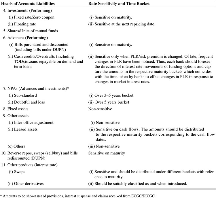
Liquidity Risk Management52
The table below shows the various facets of liquidity risk management.
GUIDANCE FOR SLOTTING THE FUTURE CASH FLOWS OF BANKS IN THE REVISED TIME BUCKETS
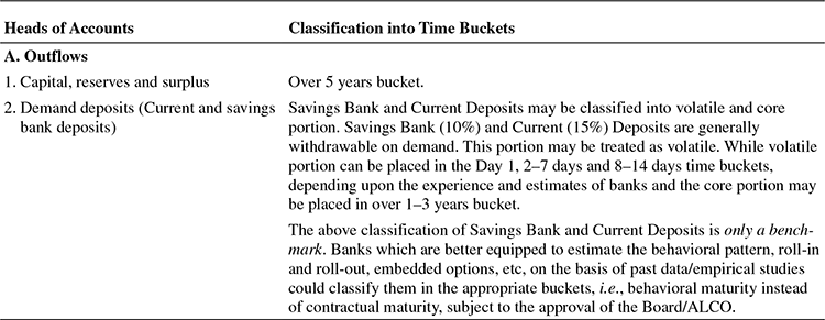
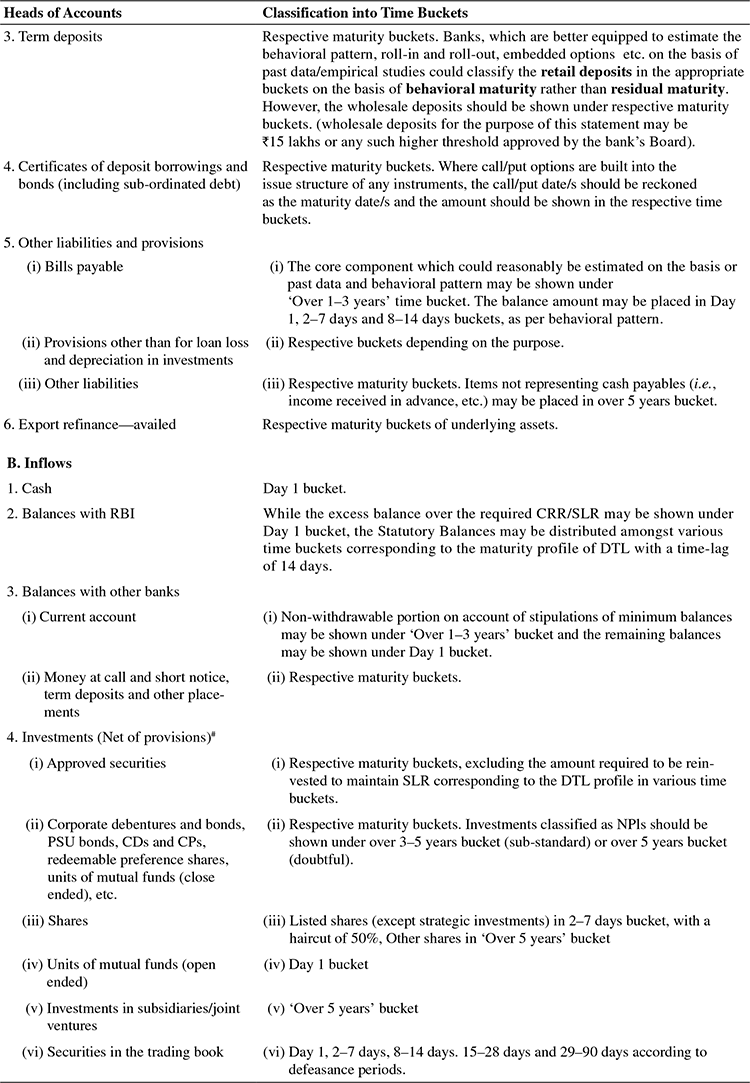

- Liability on account of event cash flow, i.e., short fall in CRR balance on reporting Fridays, wage settlement, capital expenditure, etc which are known to the banks and any other contingency may be shown under respective maturity buckets. The event cash outflows, including incremental SLR requirement should be reported against ‘Outflows–Others’.
- All overdue liabilities may be placed in the Day 1, 2–7 days and 8–14 days buckets, based on behavioral estimates.
- Interest and installments from advances and investments, which are overdue for less than one month may be placed in Day 1, 2–7 days and 8–14 days buckets, based on behavioral estimates. Further, interest and installments due (before classification as NPAs) may be placed in ‘29 days to 3 months bucket’ if the earlier receivables remain uncollected.
ANNEXURE VI
CASE STUDY—NORTHERN ROCK LIQUIDITY CRISIS
Northern Rock in July 2007 was Britain’s fifth largest mortgage lender. It had a robust credit book and analysts were positive on its medium-term outlook.
Less than 2 months later, Northern Rock collapsed. The run on Northern Rock was the first in over 100 years in the UK. Liquidity had dried up in the bank. How did it happen, so suddenly and so dramatically?
Northern Rock was not an international bank and did not have significant cross border operations. It was not a major bank either. It had been set up in 1965 as a building society, but subsequently enjoyed spectacular growth and expansion. Before the crisis, 80 per cent of the bank’s liabilities were sourced from securitizations, covered bonds and wholesale sources of funding. Retail deposits comprised only about one-fifth of the liabilities.
When the sub-prime crisis spilled over from the US into securities and money markets of other countries, Northern Rock, with its low deposit to loan ratio, was unable to renew its other sources of short-term financing. It turned to the Bank of England for ‘financial assistance’ on 14 September 2007, in view of ‘extreme conditions’ in financial markets. When the news broke, most retail customers rushed to withdraw their savings from the bank. It was reported that the UK had not witnessed such panic-driven withdrawals since 1866.
In its report, ‘The Run on the Rock’, the House of Commons Treasury Committee stated that Northern Rock was a victim of its own funding structure. Its reliance on short term, wholesale funding was responsible for its inability to cope with the liquidity pressure placed on it when the international markets dried up after the credit crisis in the US.
In February 2008, the bank was nationalized after two unsuccessful bids for take over.
During the course of all this trouble, it is noteworthy that Northern Rock did not face a problem of inadequate capital! But its vulnerability to liquidity shocks in wholesale markets proved its undoing.
A key lesson flowing from the Northern Rock debacle is that bank capital and liquidity are equally important for regulation and solvency of banks.
QUESTIONS ON THE CASE
- How is credit risk related to liquidity risk and how was this relationship manifested in the collapse of Northern Roack?
- Why was the collapse of Northern Rock described as being ‘ a victim of its (Northern Rock’s) own funding structure’?
- How can liquidity shocks occur in spite of having adequate capital?
- Has Basel III addressed the above issues? How?
ENDNOTES
- The complete report can be accessed at www.crmpolicygroup.org
- Merton, Robert C., and André F. Perold. ‘Theory of Risk Capital in Financial Firms’ Journal of Applied Corporate Finance 6, No. 3 (fall 1993): 16–32.
- Many use the term ‘market value accounting’ when evaluating how to account for a bank’s investment portfolio. But it is more than reporting investments at market value. In a technical sense, market value accounting is the valuation of an item at the price for which it can be sold. In a fundamental sense, market value accounting is the actual accounting for transactions, events and other activities at their current or fair market value instead of their original historical cost. At any particular balance sheet date, those transactions, events and other activities create both on-balance sheet and off-balance sheet assets and liabilities. Under market value accounting, these on-balance sheet and off-balance sheet assets and liabilities would be marked to market at each balance sheet date. Moreover, under market value accounting, changes in the market value of those items from balance sheet date to balance sheet date would be reported either in net income or as a separate component of stockholders’ equity.
- See Chapter on ‘Investments’ for a detailed description of VaR.
- Black, Richard, Brown, Karl, and Moloney, James, ‘Asset and Liability management: What does the future have in store?’, Balance Sheet, Volume 11, No. 2 (2003), pages 32–38.
- In general, any occasion on which interest rates are to be reset—either due to maturities or floating rate resets—is called a ‘repricing’. The date on which it occurs is called the ‘repricing date’; if a portfolio has assets repricing earlier than liabilities, it is said to be ‘asset sensitive’. This is because near term changes in earnings are going to be driven by interest rate resets on those assets. Similarly, if liabilities reprice earlier, earnings are more exposed to interest rate resets on those liabilities, and the portfolio is called ‘liability sensitive’.
- The ‘yield curve’ is a line that plots the interest rates, at a set point of time, of bonds of equal credit quality, but differing maturity dates. The benchmark yield curve compares, say, the 3 month, 2 year, 5 year and 30 year Treasury debt, and is then used to compare other debt in the market, such as home loan rates or bank lending rates. The curve is also used to predict changes in economic output and growth. The shape of the yield curve is closely scrutinized to gain an idea of future interest rate change and economic activity. There are three main types of yield curve shapes—normal (where longer maturity bonds have higher yields compared to short-term bonds), inverted (where short-term yields are higher than long-term yields, which could signal imminent recession), or flat or ‘humped’ (where short- and long-term yields are very close to one another, signifying economic transition). The slope of the yield curve is also seen as significant—the greater the slope, the greater the gap between short- and long-term rates.
- This section broadly follows the approach taken by Timothy W Koch and S Scott MacDonald in their book ‘Bank Management’, chapters 8 and 9, 4th edition, The Dryden Press, USA.
- This is easily explained if one considers that a maturing liability is a cash outflow and a maturing asset is a cash inflow.
- NIM is defined as the ratio of a bank’s NII to its earning assets.
- Macaulay’s duration and other concepts of duration are described in Annexure II.
- For more detailed discussion on ‘capital adequacy’, please see chapter titled ‘Capital–Risk, regulation and adequacy’.
- For more detailed discussion on the equity multiplier, please see chapter titled ‘Banks’ financial statements’.
- This is derived quite easily from the existing equation as follows: WADa – (MVL/MVA) WADl = 0 or, WADa – WADl + WADl – (MVL/MVA) WADl = 0 or, WADa – WADl = (MVL/MVA) WADl – WADl; the RHS can be rewritten as WADl ((MVL – MVA)/ MVA) or WADl(–MVE/MVA)
- Toevs, Aldenl (1983). “GAP Management: Managing: Interest Rate Risk in Banks and Thrifts”, pp. 30-31, Spring 1983 Economics Review, Number 2, Federal Reserve Bank of San Francisco.
- Mahshid, Deniz, and Naji, Mohammad Raiszadeh, 2003, ‘Managing interest rate risk—A case study of four Swedish savings banks’, page 30.
- See the discussion on ‘Theory of Interest Rates’ in Annexure I for better understanding of this concept.
- Hingston, Roy (2000), ‘Reducing interest rate exposure’, Community Banker, volume 9.7, pages 44–45, as quoted by Mahshid, Deniz and Naji, Mohammad Reiszadeh, 2003, ‘Managing interest rate risk—a study of four Swedish savings banks’, page 33, Master’s Thesis, Goteborg University.
- ‘Notional’ denotes that the amount of principal is used only for calculation of interest payments, and the principal as such does not change hands.
- Please see chapter on ‘Capital—Risk, regulation and adequacy’ for a detailed discussion on capital adequacy requirements for off-balance sheet positions of banks.
- For example, though the amount to be paid on its liabilities is locked in at 6 per cent in the previous example, if the market perceives higher risk over time and revises its risk premium, the bank may end up paying more on subsequent deposits.
- A ‘hedger’ is one who is willing to pay to avoid risk. Typically, a hedger has an existing or anticipated position in the ‘cash’ market, and trades futures contracts to reduce the risk arising from unexpected changes in the value of the hedger’s cash position. To elaborate further, ‘cash’ or ‘spot’ transactions represent the exchange of any asset with specific features and price between a buyer and seller, the former making payment to take possession of the asset from the latter.
- Traders are classified by their trading strategies. The ‘speculator’ assumes the risk of the ‘hedger’ in the hope of gaining from the transaction. Speculators try to guess price movements, and time their trading to sell at a price higher than the purchase price.
- Theoretically, in a market where the futures contract is priced correctly, a perfect hedge would provide a return tending to equal the risk-free rate.
- For instance, in the US, interest rate futures are traded on the Chicago Mercantile Exchange (www.cmegroup.com), one of the world’s largest and most diverse marketplaces for derivatives. Interest rate futures can be based on both short-term and long-term debt obligations. Short-term obligations are typically for less than 1 year, and those above 1 year constitute long-term obligations.
- Koch, Timothy, and Macdonald, Scott, ‘Bank Management’, Chapter 10, 4th edition, The Dryden Press.
- Arguably, futures contracts have no fixed price or cash flows, and, hence, there can be no duration ascribed to these contracts. However, research has shown that under certain assumptions, the duration of a futures contract can be assumed to equal the duration of the underlying asset.
- Saunders, Anthony, and Millon Cornett, Marcia, 2005, ‘Financial Markets and Institutions—A modern perspective’, chapter 24, 2nd edition, Tata McGraw Hill Publishing Company Ltd., India.
- Note that an ‘External Commercial Borrowing’ (ECB) raised by an Indian firm could be termed an ‘arbiloan’ if the firm’s foreign subsidiary takes a loan in its country at lower rates, converts into INR and lends it to the Indian parent. The Indian firm, in turn, has to guarantee repayment to the foreign lender.
- Based on research by Federal deposit Insurance Corporation (FDIC), 26 March 2003, ‘Derivatives Risk in Commercial Banking’.
- Bank for International Settlements, Quarterly Review, September 2009, Chapter 2 titled ‘Highlights of International Banking and Financial Markets Activity’, pages 24–25.
- FDIC, 26 March 2003, ‘Derivatives Risk in Commercial Banking’.
- International accounting standards define ‘fair value’ as the ‘value at which an asset could be exchanged or a liquidity settled between knowledgeable, willing parties in an arm’s length transaction’.
- Study conducted by Amiyatosh Purnandam, Assistant Professor of Finance at the Ross School of Business, quoted in ‘Commercial Banks Benefit by Using Derivatives for Hedging Risk’, 2005, by Claudia Capros, on the University of Michigan website, www.umich.edu
- IAS 39 is the standard pertaining to financial instruments. More information can be accessed at www.iadb.org
- This paper can be accessed at www.bis.org
- A ‘bank run’ could have a snowballing effect on the entire economy. When a large number of depositors withdraw their deposits at the same time from a bank, triggered by a fear that the bank’s assets are so eroded in value that their combined worth may not be sufficient to repay their deposits, the bank will run out of cash to repay them. If the bank recalls the loans made in a distress measure, it may realize only a part of the value of the assets, since the bank’s borrowers may be unable to pay or the securities invested in may not yield their full value.
- January, 2013, Basel Committee on Banking supervision, ‘Basel III: The Liquidity Coverage Ratio and Risk Monitoring Tools.’.
- September 2008, Basel Committee on Banking Supervision, ‘Principles for Sound Liquidity Management and Supervision’, Bank for International Settlements, page 2.
- ‘core ‘ deposits typically constitute demand deposits, savings deposits and small denomination term deposits. These deposits are looked upon as stable sources of funds, as opposed to volatile sources of funds from noncore deposits and other funding avenues.
- FDIC, The USA, 2005, ‘Risk Management Manual of Examination Policies’, Section 3.8, ‘Off balance sheet activities’ accessed at [email protected], and Bank for International Settlements, September 2008, ‘Principles for sound liquidity management and supervision’, pages 12–14.
- May 2006, The Joint Forum, Bank for International Settlements, ‘The Management of Liquidity Risk in Financial Groups’.
- September 2008, Bank for International Settlements, ‘Principles for Sound Liquidity Management and Supervision’, pages 10–30.
- The guidelines are excerpted from RBI’s ‘Draft Guidelines for improvements to banks’ Asset Liability Management Framework’, 17 April 2006. Also see Annexure 1–4 of BCBS document on interest rate risk (2004).
- It is mandatory for banks to disclose the maturity profile of their assets and liabilities in their financial statements. The classification can be found in the Notes to Accounts of banks’ financial statements.
- Note that for a zero coupon bond, the graph could be almost flat, while the graph related to coupon bonds can be quite convex.
- May 2006, The Joint Forum, Bank for International Settlements, ‘The Management of Liquidity Risk in Financial Groups’.
- The Joint Forum consists of the Basel Committee on Banking Supervision, International Organization of Securities Commissions and International Organization of Insurance Supervisors, under the aegis of the Bank of International Settlements, Basel, Switzerland.
- September 2008, Bank for International Settlements, ‘Principles for Sound Liquidity Management and Supervision’, pages 10–30.
- For the purpose of interest rate risk measurement.
- For the purpose of liquidity risk measurement.
- RBI, ‘Guidelines on Asset Liability Management (ALM) System—Amendments’ dated 24 October 2007.Source: RBI documents.