
CHAPTER NINE
Managing Credit Risk—Advanced Topics
CHAPTER STRUCTURE
Section II Select Approaches and Models—The Credit Migration Approach
Section III Select Approaches and Models—The Option Pricing Approach
Section IV Select Approaches and Models—The Actuarial Approach
Section V Select Approaches and Models—The Reduced form Approach
Section VI Pricing Credit Derivatives
Section VII The Global Credit Crisis of 2007
Section VIII A Note on Data Analytics nd Business Simulation
Annexure I Case study - The Global Credit Crisis—A Brief Chronology of Events in 2007–08
KEY TAKEAWAYS FROM THE CHAPTER
- Understand the issues in measuring credit risk.
- Understand how credit risk is measured through quantitative models.
- Find out how the popular industry sponsored credit risk models work.
- Understand how credit derivatives are priced and traded in developed markets.
- Understand how the global credit crisis happened.
- Learn about the use of ‘big data’ and business simulation.
SECTION I
BASIC CONCEPTS
Traditional methods, such as the Altman’s Z score and other credit scoring models (described in the previous chapters) try to estimate the probability of default (PD), rather than potential losses in the event of default (LGD). The traditional methods define a firm’s credit risk in the context of its ‘failure’—bankruptcy, liquidation or default. They ignore the possibility that the ‘credit quality’ of a loan or portfolio of loans could undergo a mere ‘upgrade’ or ‘downgrade’ as described in the classification of loans in the previous chapter.
The credit risk of a single borrower/client is the basis of all risk modelling. In addition, credit risk models should also capture the ‘concentration risk’ arising out of portfolio diversification and correlations between assets in the portfolio.
Recall from the previous chapter that the expected loss (EL) for a bank, arising from a single borrower or a credit portfolio is the product of three factors—Probability of default (PD), loss given default (LGD) and exposure at default (EAD).
Typically, therefore, credit risk models are expected to generate (1) loss distributions for the default risk of a single borrower and (2) portfolio value distributions for migration (upgrades and downgrades of a borrower’s creditworthiness) and default risks. It follows that all models require some common inputs, such as (1) information on the borrower(s), (2) credit exposures to these borrowers, (3) recovery rates (or LGD) and (4) default correlations (derived from asset correlations) to assess concentration risk in the credit portfolio.
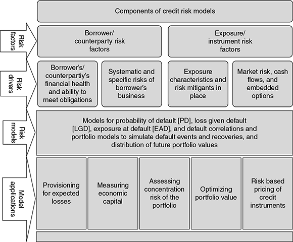
Credit risk models have a wide range of applications. They are prevalently used for
- Assessing the ‘EL’ of a single borrower.
- Measuring the ‘economic capital’1 of a financial institution
- Estimating credit concentration risk
- Optimizing the bank’s asset portfolio
- Pricing credit instruments based on the risk profile
Figure 9.1 generalizes the components of credit risk models:
FIGURE 9.1 COMPONENTS OF CREDIT RISK MODELS
Estimating PD, EAD and LGD—The Issues
Recall our discussion on ‘Loan pricing’ in an earlier chapter, where we used a simplified model to estimate the risk premium to be embedded in the loan price, analogous to the EL formula above. In that model, we had assumed that the PD had to be estimated for the borrower, taking into account various risk factors, and superimposed on the recovery rate (RR) (in the event of default), and the likely exposure of the bank to the borrower over the period (assumed as 1 year). The shortfall in the contracted rate arising out of the borrower’s default probability was called the ‘risk premium’. This was analogous to the ‘EL’ and, therefore, had to be compensated. The bank did this by simply adding the ‘risk premium’ to the loan price. In this case, we had assumed that the EAD and LGD remained constant at the estimated levels.
However, in practice, the above view is too simplistic. There are various issues in estimating the risk factors.
Let us look at each of the values that define EL.
- Assigning a PD to each customer in a bank’s credit portfolio is far from easy. One way to assess the PD is based on the fact that a default has occurred according to the bank’s internal definition or a legal definition adopted by the bank—i.e., the borrower has exceeded some default threshold. Alternatively, a credit rating migration approach can be used.
- There are two commonly used approaches to estimate default probabilities. One is to base the estimate on historical default experience—market data based on credit spreads of traded products or internally generated data, or use models, such as the KMV and others—which will be described later on in this chapter. A second approach is to associate default probabilities with credit ratings (described in an earlier chapter)—either internally generated customer ratings or those provided by external credit rating agencies, such as CRISIL (or S&P). The process of assigning a default probability to a rating is called ‘calibration’.
- The EAD is the quantity of exposure of the bank to the borrower. This is not merely the ‘outstanding’ amount in the bank’s books, as we assumed in the case of loan pricing in the earlier chapter. In fact, the EAD comprises two major parts—‘outstandings’ and ‘commitments’. The ‘outstandings’ represent the portion of the loan already drawn by the borrower, and is shown as a funded exposure on the bank’s assets. In case of default, the bank will stand exposed to the total amount of the ‘outstandings’. In the time before default, the borrower is also likely to have ‘commitments’ (undrawn portion of the bank’s promised credit limit to the borrower). These commitments can again be classified into ‘undrawn’ and ‘drawn’. Historical default studies shows that borrowers tend to draw quickly on committed lines of credit in times of financial distress. Hence, the EAD should also include the ‘drawn’ portion of the commitment at the time of default. Since the borrower has the ‘right’ but not the ‘obligation’ to draw on undrawn commitments (the embedded ‘option’), we can consider the proportion of drawn to undrawn commitments as a random variable. Therefore, now EAD becomes the aggregate of the outstanding exposure + a fraction of the undrawn commitment likely to be drawn prior to default. In practice, banks will calculate this fraction as a function of the borrower’s creditworthiness and the type of credit facility.
- One approach to estimate EAD is to assume it as being equal to ‘current exposure + ‘Loan Equivalency Factor (LEF)’ × unutilized portion of the limit’.2 The LEF is the portion of the unutilized credit limit expected to be drawn down before default, and depends on the type of facility and the credit rating just before default, as stated in the preceding paragraph. The cited World Bank paper provides a simple method to approximate LEF as shown in Figure 9.2.3
- In the case of derivatives, the potential future exposure depends on the movement in the credit quality/value of the underlying asset, and this is estimated using simulation techniques.
FIGURE 9.2 ONE METHOD OF APPROXIMATING LEF
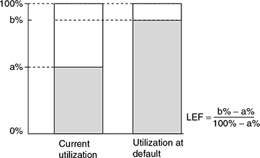 Source: Wold Bank Policy, Research Working Paper.
 - Modelling EAD should also take into account the ‘covenants’ attached to the loan document. Most of these covenants represent ‘embedded options’ for the borrower or the bank. For example, a covenant may require that the borrower provides additional collateral security in times of impending financial distress. In such a case, the borrower firm will have more information about its likelihood of default than the bank, which watches for signals of incipient distress (as described in an earlier chapter). In cases where banks are permitted by the covenants to close undrawn commitments based on predefined early indicators of default, the banks have to move quickly before the borrower draws on the undrawn commitments. This aspect will be discussed in detail in the subsequent chapter on ‘Capital Adequacy’ and the Basel Committee regulations.
- The LGD is simply the proportion of EAD lost in case of default, and is typically estimated as (1–recovery rate)—i.e., the actual ‘loss’ to the bank in case of default by the borrower. However, recovery rate (RR) is not static—it depends on the ‘quality’ of the collaterals (in case of decline in economic growth, the value of these securities could decline) and the ‘seniority’ of the bank’s claim on the borrower’s assets. Additionally, ‘recovery’ could also entail ‘financial cost’ (such as interest income lost due to time taken for recovery or the cost of ‘workout’ as discussed in a previous chapter). In reality, therefore, the LGD is modelled as the ‘expected severity’ of the loss in the event of default.
- According to Schuermann,4 there are three broad methods to measure LGD.
- Market LGD, which can be computed directly from market prices or trades of defaulted bonds or loans;
- Workout LGD that depends on the magnitude and timing of the cash flows (including costs) from the workout process. LGD can be computed under this method as EAD less recovery plus workout costs incurred expressed as a percentage of EAD. Since the recovery process can be long winded, the cash flows should be expressed in present value (PV) terms. The question then arises as to what the appropriate discount rate should be. According to Schuermann, the discount rate could be that for an asset of similar risk, or the bank’s own hurdle rate. In practice, workout LGD is the most popular, especially with banks with prior experience in such defaults; and
- Implied Market LGD that is derived from prices of fixed income and credit derivatives, using a theoretical asset pricing model.
- Approaches to modelling LGD are evolving rapidly. The initial models identified the factors driving the LGD values, including the correlation between PD and LGD. Schuermann’s paper quoted above belongs to the ‘first generation’ models, as does Altman (et al)’s 2005 paper.5 The ‘second wave’ of models developed and empirically applied frameworks to quantify the correlation between PD and LGD. The current stream of models derives concepts to stress LGDs in economic downturns, as in the events happening since 2007. There is a need to now calculate a ‘downturn LGD’ (BLGD). The Basel committee on Banking Supervision has proposed such a model in its 2006 comprehensive version of the revised framework,6 and the Federal Reserve uses a simple model to arrive at the BLGD7:
BLGD = 0.08 + 0.92 ELGD
where ELGD is the ‘expected LGD’.
The above linear relationship between BLGD and ELGD, however, does not take into account the degree to which the risk segments are exposed to ‘systematic risks’.
Why Do We Need Credit Risk Models?
There are important differences between market risk 8 and credit risk. While market risk is the risk of adverse price movements in equity, foreign currency, bonds, etc., credit risk is the risk of adverse price movements due to changes in credit events, such as borrower or counter party defaults or credit rating downgrades. These risks are also called ‘market VaR’ and ‘credit VaR’, the term VaR denoting ‘Value at Risk’, a technique to measure risk.
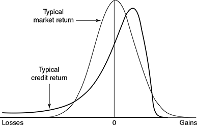
First, the portfolio distribution for credit VaR hardly conforms to the normal distribution. Credit returns tend to be highly skewed—while lenders’ benefits are limited when there is an upgrade in credit quality, their losses are substantial in the case of downgrade or default, as shown in Figure 9.3.
Second, market VaR can be directly calculated based on daily/periodic price fluctuations. However, measuring portfolio effect due to credit diversification is more complex than for market risk. To measure this effect, estimates of correlations in credit quality changes among all pairs of borrowers/counter parties have to be obtained. However, these correlations are not readily observable, and several assumptions are required for such correlation estimates.
Third, though the default probability of a borrower or counter party can be likened to ‘asset volatility’ in market risk, credit risk is more complicated. Take the instance of currency risk, an important market risk. One of the ways of arriving at the rate volatility is to observe the fluctuations in the currency over a period of time, and compute a reasonable estimate of the currency’s volatility. However, a borrower’s history may indicate nothing about the probability of future default; in fact, in many cases, the very fact that the lender stays exposed to the borrower signifies no prior default!
Credit risk models are valuable since they provide users and decision makers with insights that are not otherwise available or can be gathered only at a prohibitive cost. A credit risk model should be able to guide the decision-making manager on allocating scarce capital to various loan assets, so that the bank’s risk-return trade off is optimized. Optimization, of course, does not imply ‘risk elimination’—it means achieving the targeted or maximum return at minimum risk.
Banks typically have a diversified portfolio of assets. Most credit risk models compare risk-return characteristics between individual assets or businesses in order to quantify the diversification of risks and ensure that the bank is well diversified.
A good credit risk management model is expected to generate the outputs as given in Figure 9.4.
FIGURE 9.4 OUTPUTS OF A CREDIT RISk MODEL
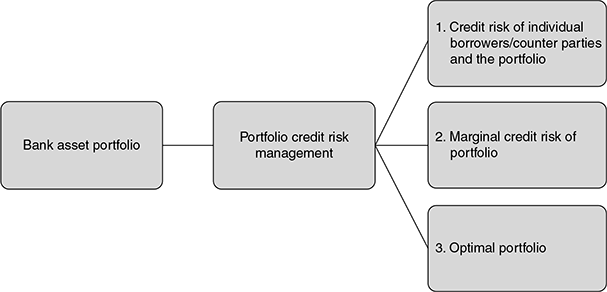
- Credit risk of portfolio in Figure 9.4 indicates the output defining the probability distribution of losses due to credit risk.
- The marginal credit risk of the portfolio in Figure 9.4 depicts how the risk-return trade off would change if an incremental (marginal) asset is added to the portfolio. This output helps bank managers to decide on new investment options for the bank and the price that can be paid for the opportunity.
- The optimal portfolio is the optimal mix of assets that the bank should have at that point in time.
Every credit risk model is built on certain assumptions and, therefore, may not be able to generate all the outputs as above. Further, they cannot be used mechanically for predictions, since they are constructed mostly out of historical data. The outputs of the models are useful tools for decision making, but cannot substitute judgment and experience of bank managers.
Credit Risk Models—Best Practice Industry Models
Credit risk has been recognized as the largest source of risk to banks. The increasing focus of measuring credit risk through models—internal to banks and industrysponsored—can be attributed to the following:
- Substantial research has been carried out and advanced analytical methods have been evolved for formulating and implementing credit risk models;
- The ‘economic capital’ of a bank is aligned closely to the bank’s credit risk. Hence, efficient allocation of capital within a bank presupposes accurate quantification of credit risk, and better understanding of the impact of credit concentration and diversification on the bank’s asset portfolio on the bank’s capital requirements.9
- The other incentives flowing from credit risk measurement include better pricing of credit due to better valuation of financial contracts, and better management of funds, due to accurate assessment of risk and diversification benefits.
- Regulatory developments, such as the Basel II Capital Accord10 have necessitated use of risk models.
The previous chapter lists some industry-sponsored credit risk models, based on approaches, such as the ‘credit migration approach’, ‘option pricing approach’, (these two classes of models are called ‘structural models’), the ‘actuarial approach’ and the ‘reduced-form approach’.
The above models can also be classified as given in Figure 9.5. This classification is based on the approach adopted by the model for credit risk measurement.
FIGURE 9.5 CLASSIFICATION OF SOME INDUSTRY-SPONSORED BEST PRACTICE CREDIT RISK MODELS
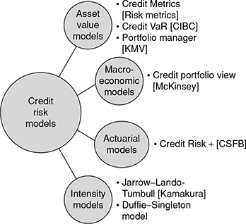
In the following sections, we will provide an overview of each of the above approaches.
SECTION II
SELECT APPROACHES AND MODELS—THE CREDIT MIGRATION APPROACH
The Credit Migration Approach (Used by Credit MetricsTM11)
We have seen that credit quality can vary over time. ‘Credit migration’ is analyzed as the probability of moving from one credit quality to another, including default, within a specified time horizon, usually a year.
‘Credit Metrics™’, the most well-known credit migration model, builds upon a broad body of research12 that applies migration analysis to credit risk measurement. The model computes the full (1 year) forward distribution of values for a loan portfolio, where the changes in values are assumed as due to credit migration alone, while interest rates are assumed to evolve in a deterministic manner. ‘Credit VaR’13 is then derived as a percentile of the distribution corresponding to the desired confidence level.
Though we have earlier drawn the distinction between ‘market’ and ‘credit’ risks in order to isolate them and deal with them, the real world picture is different. For example, credit risk could arise due to volatility in currency movements, in which case, we have to capture market risk components as well in the credit risk models. The credit risk models are being increasingly refined to account for the impact of market risks.
However, as a first step, it would help to understand how the basic credit migration approach works for measuring credit risk.
Step 1: Assessing Real World Probabilities of Default—The Transition Matrix Credit rating agencies periodically construct, from historical data, a ‘transition matrix’, which shows the probability of an existing (rated) loan getting upgraded or downgraded or defaulting during a specified period in time (typically 1 year). The matrix is usually presented in the way as shown in Table 9.1. (in the case of S&P, CRISIL14):
TABLE 9.1 CRISIL’S AVERAGE 1-YEAR TRANSITION RATES

Each cell in the above matrix contains a probability. The rating categories in the columns of the matrix signify the expected credit rating 1 year in the future. The rating categories in the rows of the matrix show current credit ratings.
For example, the probability in the cell AA-AAA will signify the chances of a loan, currently assigned an AA rating, upgrading to AAA over the ensuing year. Similarly, the probability in the cell A-BBB will signify the chances that a loan, currently rated A, downgrades to BBB over the next 1 year. The highlighted cells AAA-AAA, AA-AA and so on, therefore, signify the probability that the loan stays in the same category. These probabilities are ‘real world probabilities’15 as they have been calculated from historical data. For example, the transition matrix given by CRISIL in the reference provided has been constructed out of data over the period 1992–2007.16
Box 9.1 explains the distinction between ‘real world’ and ‘risk neutral’ probabilities, and their usage in credit risk analysis.
BOX 9.1 REAL WORLD VERSUS RISK NEUTRAL PROBABILITIES
TABLE 9.2 shows the average cumulative default rates estimated by CRISIL17 for rated credit instruments.
TABLE 9.2 CRISIL AVERAGE CUMULATIVE DEFAULT RATES (WITHDRAWAL-ADJUSTED)

From Table 9.2, we can infer that the probability of an A-rated loan defaulting in 1 year is.42 per cent, in 2 years is 1.03 per cent and in 3 years is 1.97 per cent. These are ‘real world’ probabilities, estimated from historical data—in the above case, data from 2000 to 2007.
Now let us assume that an A-rated loan is priced 100 bps (fixed) over the bank’s Prime lending rate (the rate at which it lends to ‘risk free’ borrowers). Assuming a zero RR from the loan in case of default, the PD would be given by the equation 1 – [1/(1 + r)n], where r denotes the premium over the risk-free rate and n the number of periods. Using this equation, the estimated probabilities of default would be 1 per cent, 1.97 per cent and 2.94 per cent for 1, 2 and 3 years, respectively.
Compare these probabilities with the historical probabilities of default in Table 9.2. Are the results inconsistent? They are not.
To understand the concept, we should note that the value of a risk-free loan is higher than the value of an Arated loan that carries some element of risk. In other words, (1) the expected cash flow from the A-rated loan at the end of 3 years would be 2.94 per cent less than the expected cash flow from a risk-free loan at the end of 3 years, and (2) both cash flows would be discounted at the same rate in a risk neutral world, i.e., at the prime lending rate or riskfree rate.
The above is analogous to stating that (1) the expected cash flow from the A-rated loan at the end of 3 years is 1.97 per cent less than the expected cash flow from a risk-free loan at the end of 3 years, and (2) the appropriate discount rate for the A-rated loan’s expected cash flow is about 0.32 per cent higher than the discount rate applicable to the risk-free loan’s cash flow—because a 0.32 per cent increase in the discount rate leads to the A-rated loan’s value being reduced by the difference between the risk neutral and real world PD, i.e., 1.97 per cent and 2.94 per cent, which is 0.97 per cent over 3 years or 0.32 per cent per year.
It, therefore, follows that 1.97 per cent is a correct estimate of the real world PD, if the correct discount rate to be used for the debt cash flow in the real world is 0.32 per cent higher than in the risk neutral world. The increase in the discount rate seems reasonable as A-rated loans have been perceived to have higher systematic risks—when the economy does badly, they are more likely to default.18
The question, therefore, is—which PD is appropriate for credit risk analysis—the real world or the risk neutral one?
Typically, analysts use risk neutral default probabilities while pricing credit derivatives or estimating the impact of credit risk on the pricing of instruments such as in the calculation of the PV of the cost of default (since risk neutral valuation is commonly used in the analysis). Real world probabilities are commonly used in scenario analysis as for estimating Credit VaR (to estimate potential future losses in the event of default).
The information contained in transition matrices provided by renowned credit rating agencies is considered robust and useful and is being used as the starting point for modelling credit risk. However, there are certain criticisms, the most obvious of them being that these transition probabilities only reflect averages over several years, and lack the predictive ability to determine how serious or benign the forthcoming year’s credit transitions would be. To address this shortcoming, smaller historical periods are sometimes chosen to reflect the most likely current scenario, and transition matrices constructed. Another method used to improve the predictive ability is to model the relationship between transition of credit defaults and select macroeconomic variables, say, industrial production.
However, it has to be recognized here that predicting the PD or downgrade/upgrade in credit quality is a difficult task in practice. Hence, it would be prudent to stress test the portfolio under a variety of transition assumptions.
In many cases, banks develop their own transition matrices based on their borrowers’ profile, since the probabilities provided by rating agencies are average statistics obtained from a heterogeneous sample of firms, with varying business cycles.
Step 2: Specifying the Credit Risk Horizon The risk horizon is typically taken to be 1 year, as assumed by the transition matrix. This is a convenient assumption, but can be an arbitrary one.19 It should be noted here that the transition matrix should be estimated for the same time interval over which the credit risk is being assessed. For example, a semi annual risk horizon would use a semi annual transition matrix.20
Step 3: Revaluing the Loan In this step, we calculate the value of the loan at the end of the risk horizon. However, since there are eight possible ratings in the transition matrix, we have to estimate eight values of the same loan. This estimation has to be done within two broad, mutually exclusive assumptions.
- In the worst case, if the loan defaults over the horizon, some recovery would be possible based on the available collaterals.
- Alternatively, the loan can simply move between the ratings—an ‘upgrade’ or a ‘downgrade’. In the second case, we need to revalue the loan based on the rating to which it migrates.
Assume that credit risk is being assessed for one large, long-term loan.
- In the worst case of default, we require two important inputs—the ‘seniority’ of the loan and the ‘recovery’ in case of default. The likely value of the loan will depend on how much can be recovered, say, by enforcing securities offered for the loan, which, in turn will depend on the ‘seniority’ of the loan, the mean recovery rate and the volatility (standard deviation) of the RR. The Credit Metrics technical document provides the Table 9.321:
TABLE 9.3 RECOVERY RATES BY SENIORITY CLASS (PER CENT OF FACE VALUE—‘PAR’)
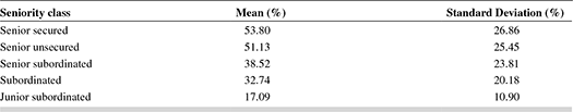 Source: Carty and Liberman [96a]—Moody’s Investors Service
Table 9.3 can be interpreted easily. If the loan or bond is ‘senior secured’, its mean recovery in default would be 53.8 per cent of its face value, i.e., for a loan of, say, ₹100 crore, the average recovery would be ₹53.80 crore, with a volatility (standard deviation) of 26.86 per cent.
See BOX 9.2 for further discussion on the relationship between the PD and recovery rates.
BOX 9.2 RELATIONSHIP BETWEEN PROBABILITY OF DEFAULT AND RECOVERY RATE
From our discussion earlier in this chapter, we know that EL under credit risk is calculated as the product of three factors—PD, LGD and EAD. RR is 1 – LGD.
While credit risk literature abounds with work on estimating PD, much less attention has been devoted to estimation of RR and its relationship with PD22. However, empirical evidence seems to suggest that: (1) recovery rates can be volatile; and (2) they tend to decrease (or LGDs increase) when PD increases, say, due to economic downturns.
However, many credit risk models continue to work with simplifying assumptions based on static losses for a given type of debt as in Table 9.3. It should also be noted that credit VaR models such as the one being discussed, treat RR and PD as two independent variables.
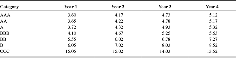
- b. In case of an expected upgrade or downgrade in credit rating, i.e., if a BBB-rated loan moves up to A or moves down to BB over the risk horizon, the ‘value’ of the loan would also change. The magnitude of this change can be assessed by estimating the forward zero curves23 for each rating category, stated as of the risk horizon, going up to the maturity of the loan. Table 9.4 shows a sample of 1-year forward zero curves by rating category.24
We can now revalue the loan using forward rates as above, and the promised cash flows from the loan over the risk horizon for the appropriate rating category. The result of this exercise would be a distribution of loan values over all the rating categories.
TABLE 9.4 EXAMPLE 1-YEAR FORWARD ZERO CURVES BY CREDIT RATING CATEGORY (PER CENT)
Step 4: Estimating Credit Risk The probabilities of migration of a single-rated loan to other categories from Step 1, and the result of the calculation in Step 3 would enable us calculate the expected value (mean) of the loan over the risk horizon, as well as the volatility (standard deviation). This standard deviation is the measure of ‘credit risk’ of the loan.
Another way to estimate the credit risk is to use ‘percentile levels’. For example, if we determine the 5th percentile level for the loan portfolio, it denotes the level below which the portfolio value will fall with probability 5 per cent. For large portfolios, percentile levels are more meaningful. This is also called the Credit VaR.
Illustration 9.1 clarifies the methodology through a numerical example.
ILLUSTRATION 9.1
Estimating the credit risk of a single loan exposure
The problem
Using the Credit Migration approach, calculate the Credit Risk (Credit VaR) of a senior secured loan of ₹100 crore, to be repaid in 5 years, at an annual interest rate of 10 per cent.
Key inputs and assumptions
- Risk horizon is 1 year
- CRISIL’s credit transition matrix given in Table 9.1 will be used.
- The current credit rating for this senior secured loan is ‘A’
- The recovery rates and the 1-year forward zero curves as given in step 3 above would be used in the calculations
- For calculation convenience, it can be assumed here that the principal is paid at the end of 5 years, while the annual interest of ₹10 crore is paid every year.
Step 1 Using the transition matrix, recovery rates and the forward curves given above, we will estimate the credit risk of the loan over the risk horizon.
We first determine the cash flows over the loan period—₹10 crore every year at the end of next 4 years as interest, and ₹110 crore at the end of the 5th year, including principal payment. This is similar to a straightforward bond valuation. The Credit Metrics document mentions that, among others, the methodology is applicable to bank loans as for bonds.
Using the forward rates applicable to an A-rated loan, we determine the value of the loan over the risk horizon. The discount rates are taken from the earlier 1-year forward zero curve as applicable to an A-rated instrument, and calculated as follows:
That is, loan value = ₹126.89 crore over the next 1 year
Now let us calculate the value of the loan, assuming it downgrades to BBB. The loan value will be calculated as follows:
That is loan value now changes to ₹125.67 crore, showing erosion in value due to the downgrade.
Continuing this exercise for all rating categories, we arrive at the possible 1 year forward values of the loan for all rating categories as in Table 9.5.
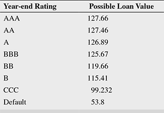
The default value is the mean value in default for a senior secured loan of ₹100 crore (53.8 per cent of ₹100 crore) as given in Table 9.3 containing recovery rates. Also from the same table, the standard deviation of the RR is 26.86 per cent.
Step 2 With the above inputs, we can calculate the volatility in loan value due to credit quality changes, using Table 9.6. Note that the probabilities of rating migrations have been obtained from CRISIL’s transition matrix in Table 9.1.
TABLE 9.6 VOLATILITY IN LOAN VALUE DUE TO CREDIT RATING CHANGES

We have now obtained one measure of credit risk—the standard deviation. The mean is calculated as an expected loan value using the probabilities of migration, and the standard deviation measures the dispersion of the likely loan values from the mean. ₹7.38 crore is, therefore, one measure of the absolute amount of the credit risk in the loan of ₹100 crore.
However, this value of credit risk has not taken into consideration the volatility (standard deviation) in the recovery rate. The RR in case of default was assumed to be the mean value of ₹53.80 crore, but this amount of recovery is uncertain since the volatility was estimated at 26.86 per cent. This uncertainty has to also find a place in our estimate of credit risk. The Credit Metrics technical document uses the following formula to include the volatility in RR in case of default25:
Accordingly, the standard deviation of the default state is included in the calculation. In the other cases of downgrade and upgrade, this volatility is assumed to be 0. This implies that in Table 9.6, the last term under ‘D’, 46.44, should be added to the product of the PD (.009) and the square of the standard deviation of default, that is, 26.862. This yields a higher standard deviation of ₹7.81 crore, amounting to a 5.7 per cent increase in volatility.
The revised Table 9.7 is shown as follows:
TABLE 9.7 REVISED VOLATILITY
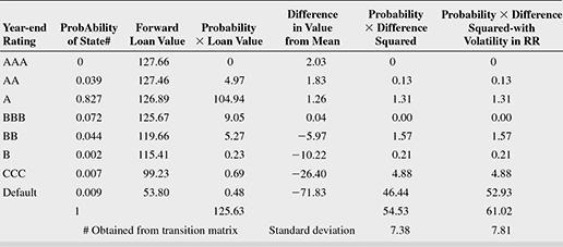
We should note here that we have considered the volatility of only the RR in case of default to arrive at a measure of the credit risk. This implies that we are assuming that there is zero volatility or uncertainty in the upgrade and downgrade states. However, this cannot be true in a practical situation—the volatility in each rating would be determined by the credit ‘spreads’ within each rating category. (The Credit Metrics technical document is aware of this shortcoming, arising out of non-availability of data to determine what portion of the credit spread volatility is due to ‘systematic’ factors, and what portion is diversifiable.)
Calculating credit risk using the percentile level—the credit VaR
If we want to ascertain the level below which our loan value will fall with a probability of say, 1 per cent, we can use the values generated by Table 9.7. Let us move upwards in the probability column (generated by the transition matrix), stopping at the point where the probability becomes 1 per cent. In our transition matrix, we see that for an A-rated loan, the PD is 0.9 per cent, and the probability that it moves to CCC is 0.7 per cent. The joint probability of being in default or in the CCC state is, therefore, 1.6 per cent, which is more than 1 per cent. Hence, we read off the value from the CCC row—99,33. This is the first percentile level value, which is ₹26.40 crore lower than the expected (mean) loan value.
Calculating credit VaR
The changes in the forward value of the A-rated loan is shown in Table 9.8.
TABLE 9.8 CHANGES IN FORWARD VALUE OF THE LOAN
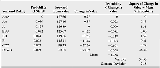
We can see that this distribution of changes in loan value under various rating changes shows long downside tails, the variance and standard deviation of the distribution remaining the same. In the earlier paragraph, we calculated the first percentile at 99.23. The corresponding first percentile of the distribution of change in loan value is –27.66, which is the credit VaR.
(However, if we assume a normal distribution for the change in loan value distribution, the credit VaR at the first percentile would be much lower at –18.46)26
Model Applied to Loan Commitments
In the above example, a loan had been treated as a zero coupon bond to arrive at the Credit VaR. However, loans may not be drawn fully upto the sanctioned limit. Also, most loans pay a portion of the principal along with the required interest payments.
We have seen in earlier chapters that a loan commitment is composed of a drawn and undrawn portion. The drawdown on the loan commitment is the amount currently borrowed. Interest is paid on the drawn portion, and a fee is paid on the undrawn portion. This fee is called a commitment fee. When we revalue a loan commitment given a credit rating change, we must therefore account for the changes in value to both portions. The drawn portion is revalued exactly like a loan. To this we add the change in value of the undrawn portion.
Since loan commitments give the borrower the option of changing the size of a loan, the commitments can dynamically change the portfolio composition. The amount drawn down at the risk horizon is closely related to the credit rating of the borrower. For example, if a borrower’s credit rating deteriorates, it is likely to draw down additional funds. On the other hand, if its prospects improve, it is unlikely to need the extra borrowings.
The worst possible case is where the borrower draws down the full amount and then defaults. This is the simplest approach, and from a risk perspective, the most conservative. In practice, it has been seen that commitments are not always fully drawn in the case of default, and hence, that the risk on a loan commitment is less than the risk of a fully drawn loan. In order to model commitments more accurately, it is necessary to estimate not only the amount of the commitment which will be drawn down in the case of default, but also the amount which will be drawn down (or paid back) as the borrower undergoes credit rating changes.
The methodology for credit VaR estimation of loan commitments is described in the technical document.27 It can be seen that the methodology is an extension of that used in Illustration 9.1. The technical document also provides methodologies for Letters of Credit (LC – described in other chapters in this book) and market driven instruments such as derivative instruments (also called Counterparty Credit Risk-CCR).
Calculation of Portfolio Risk28
The methodology in the Illustration 9.1 can be extended and employed to assess the credit risk in a portfolio of loans with the bank. The approach is described in detail in the Credit Metrics technical document.
In brief, the methodology for a two loan portfolio would be as follows:
Step 1 Describe the basic features of both loans—their tenor, credit rating, amount and interest rate.
Step 2 Describe the transition matrix and the risk horizon—the same transition matrix can be used. The risk horizon has to be the same for the portfolio being described.
Step 3 Just as in the one loan case above, we need to specify the year end values for both loans using the relevant forward rate curves, and the probabilities of achieving these values (from the transition matrix).
Step 4 Calculate joint probabilities for all rating categories—if there are eight rating categories, the matrix will have 8 × 8 = 64 values—each reflecting a joint probability for the loans. The joint probability is calculated simply by multiplying individual probabilities for each scenario. For example, the joint probability that two loans retain their original ratings is the product of the probabilities that each retains its original rating.
Step 5 The two loans can be revalued as in the single loan case above, and then combined as the sum of individual values for each rating class. There would be 64 such combined values (assuming eight rating categories).
Step 6 The portfolio standard deviation is calculated in the same manner as for a single loan. However, there will now be 64 probability states against 8 in the single loan case. The percentile level can also be computed in a manner similar to the case of a single loan.
Step 7 However, the above method of calculating joint probabilities will be valid only for those cases where the loans/assets are not correlated. If there is any kind of dependence between the borrowers, the method of calculating joint probabilities will have to take the correlation into consideration. It has been shown that the overall credit VaR is quite sensitive to correlations, which could arise from borrowing firms being in the same industry/sector, or vary with the state of the economy. Hence, where asset returns are correlated, joint migration probabilities have to be arrived at. To achieve this, Credit Metrics estimates the correlations between equity returns of the two borrowers. It has to be noted here that equity returns are being used as a proxy for asset returns, since asset returns are not directly observable. In effect, this is equivalent to assuming that the firm is entirely financed by equity.
Step 8 Assuming that the joint normalized return distribution is bivariate normal,29 arrive at the credit quality thresholds for each credit rating in the transition matrix. The same procedure is repeated for arriving at the joint rating probabilities for all combinations in the transition matrix related to the two borrowers.
Step 9 The probability of joint defaults as a function of asset return correlations is then obtained.
The above procedure, as well as the Monte Carlo simulation that is used in practice for large portfolios, is described in detail in the Credit Metrics technical document.
Credit Manager—We have seen in the earlier chapter that the interplay of credit and market risks is a significant source of risk to banks. Risk Metrics has devised the Credit Manager to deliver portfolio credit risk management across multiple asset classes, such as bonds, credit derivatives and traditional credit exposures. The methodology is similar to the Credit Metrics methodology described above.
Counter party credit exposure models—We have also seen earlier the influence of counter parties on credit risk. A counter party default would have consequences similar to borrower default. One challenge in arriving at exposures in respect of counter parties is the way OTC transactions are structured or customized. For example. Estimation of credit exposure to derivatives counter parties involves issues such as (a) determination of the replacement cost of a particular transaction at a given point in time involves modeling risk factors, and pricing the instrument; (b) modeling netting and margining arrangements between counter parties; (c) consolidation of exposures at any level of the portfolio to enable limit and exposure management, and so on. Risk Metrics’ counter party credit exposure models aim to address a broad spectrum of risks.
Details on the above models can be accessed at www.msci.com
The Credit Migration Approach (Used by CreditPortfolioView)
Credit Portfolio View (CPV) was developed by McKinsey and Company based on two papers by Thomas C Wilson30, then Principal consultant at McKinsey and company.
In summary, CPV is a ratings-based portfolio model used to define the relationship between macroeco nomic cycles and credit risk in a bank’s portfolio. It is based on the observation that default and migration probabilities downgrade when the economy worsens (i.e., defaults increase), and the contrary happens when the economy strengthens. The model simulates joint conditional distribution of default and migration probabilities for non-investment grade (non-IG) borrowers (whose default probabilities are more sensitive to credit cycles, which are assumed to follow business cycles closely, than those of highly rated borrowers) in different industries and for each country, conditional on the value of macroeconomic factors, such as follows:
- Unemployment rate
- GDP growth rate
- Level of long-term interest rates
- Foreign exchange rates
- Government expenditure
- Aggregate savings rate
CPV calls these ‘conditional migration probabilities’ for a particular year, since it is constructed conditional on the economic conditions of that year. It should be noted here that the previous model, Credit Metrics, used ‘unconditional migration probabilities’, which is the average of conditional probabilities sampled over several years.
Thomas C Wilson31 points out that this approach differs from others in that it models the actual, discrete loss distribution (as opposed to using normal distributions or mean variance approximations); the losses or gains are measured on a default/no default basis for illiquid credit exposures as well as liquid secondary market positions, and retail lending, such as mortgages and overdrafts; the loss distributions are driven by the state of the economy, since most of the systematic risk in a portfolio has been found to arise from economic cycles; and the approach is based on a multi-factor systematic risk that is closer to reality, while other models capture default correlations based on a single systematic risk factor.
The model follows three essential steps:
Step 1 Determine the state of the economy.
Step 2 Estimate the PD of customers/customer segments.
Step 3 Arrive at the loss distribution.
Illustration32 9.2 would help in understanding the methodology through a simple numerical example.
ILLUSTRATION 9.2
Credit portfolio view basic methodology
(Based on Thomas Wilson’s paper-portfolio credit risk—October 1998)
Step 1 The states of the economy
| State | GDP | PD% |
|---|---|---|
| Growth | 1 | 33.33 |
| Normal | 0 | 33.33 |
| Recession | 21 | 33.33 |
Step 2 Assume two customers/customer segments, X and Y, for simplicity
Customers have different risk profiles
| State | Customer X—Medium Risk—PD | Customer Y—High Risk—PD |
|---|---|---|
| Growth | 2.5 | 0.75 |
| Normal | 3 | 3.5 |
| Recession | 4.5 | 5 |
Note that we assume that the high-risk customer has lower
likelihood of defaulting when the economy is growing.
Step 3 Arrive at the loss distribution
There are four possibilities in each state of the economy—X defaults, Y defaults, both X and Y default, or there is no default
Assume loss in case of default as ₹100 in the case of both X and Y
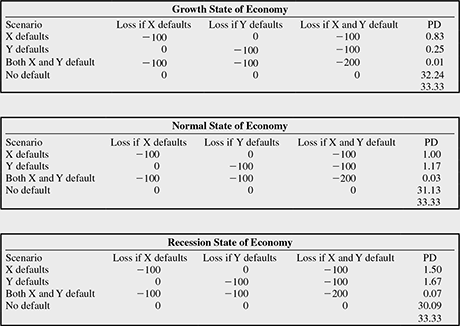
Here, we have assumed that X and Y are independent of each other, that is, correlation = 0
FIGURE 9.6 PROBABILITY OF LOSS ACROSS ALL STATES OF THE ECONOMY
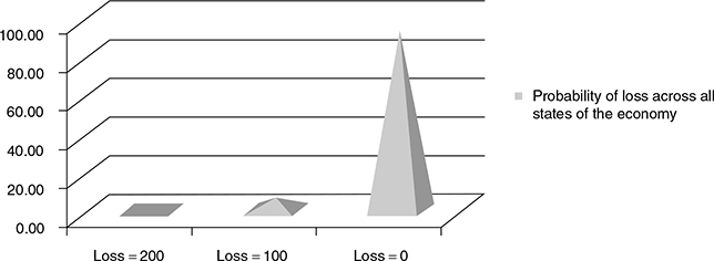
It can be seen from the above simple example that the ‘conditional’ probability of, say, a ₹200 loss in the growth state of the economy is 0.01 per cent, while, from the above graph the ‘unconditional’ loss of ₹200 across all states in the economy has a probability of 0.12 per cent.
Thus, ignoring the effect of the economy (systematic risk), it appears that X and Y are correlated. However, if the economic state is considered, the PD of X and Y as well as the joint conditional PD for X and Y is seen to be significantly higher during times of recession than during economic growth. This would imply more correlated defaults during recessionary periods, rather than an overall correlation between defaults of X and Y arising from the presence of both systematic and non-systematic risks.33
Therefore, the basic premise of the CPV is that credit migration probabilities show random fluctuations due to the volatility in economic cycles. It also assumes that different ‘risk segments’ into which borrowers are classified (in the above example, ‘X’ is a ‘risk segment’ and so is ‘Y’, and a bank can classify its borrowers into varying risk segments that could correspond with the ‘ratings’ given in the migration matrix in the previous example on Credit Metrics) react differently to economic conditions.
If we assume X and Y to be large ‘risk segments’ of borrowers whose non-systematic risks have been diversified away, then the systematic risks alone have to be considered to arrive at joint default correlations. Though this assumption is made implicitly by other models, this model extends the standard single factor approach to a multi-factor approach to capture country- and industry-specific shocks.
For each ‘risk segment’, CPV simulates a ‘conditional migration matrix’ as done in the simple numerical example above. Hence, in the three different ‘states of the economy’ envisaged in the ‘risk horizon’ (say, 1 year), the migration matrix will exhibit different characteristics, as in the simple two borrower example above: (1) in the ‘growth state’, it is likely that there are a lower number of probable downgrades and higher upgrade probabilities; (2) in the ‘normal state’, the conditional migration matrix is likely to be similar to the ‘unconditional migration matrix’ derived from historical observations (i.e., similar to the migration matrix shown in the Credit Metrics example); and (3) in the ‘recession state’, the downgrades are more likely than upgrades. This concept of ‘segment-specific risk’ for each macro economic scenario gives the CPV flexibility to simulate a ‘systematic risk model’ with a large number of such scenarios and migration possibilities.
In practice, CPV uses simulation tools, such as ‘Monte Carlo’ methods to generate a systematic risk model and simulates the conditional default probabilities for each risk segment, using two different methods of ‘calibration’34—CPV Macro and CPV Direct.
CPV Macro uses a ‘macroeconomic regression model’ using time series of historical data on macroeconomic factors, as described by Wilson in his papers quoted above.
CPV Direct was developed later to make the calibration easier, and derives default probabilities from a ‘gamma distribution’.35
Finally, all conditional loss distributions are aggregated to arrive at the unconditional loss distribution for the portfolio. The technical documentation for CPV is not available freely, and will have to be obtained from McKinsey and company.
SECTION III
SELECT APPROACHES AND MODELS—THE OPTION PRICING APPROACH
The KMV36 Model
The models discussed above have made three critical assumptions: (1) all borrowers included in a specified rating category carry the same default risk, (2) the actual default rate within a rating category would be the same as the historical default rate that has been observed over the years, and (3) all borrowers within each rating category carry the same PD or migration. These assumptions may not be totally valid in real world situations.
The KMV model strongly refutes these assumptions on the following grounds: (1) default rates are continuous, while ratings are adjusted in a discrete fashion by rating agencies; (2) rating agencies take time to upgrade or downgrade borrowers/counter parties, and such credit quality changes would be carried out at some point in time after the default risk is observed.
Further, KMV has demonstrated through simulation exercises that (a) the historical average default rate and transition probabilities can deviate significantly from the actual rates, (b) that substantial differences in default rates may exist within the same rating class, and (c) the overlap in default probability ranges may be quite large. In some cases, the historical default rate could, in reality, overstate the actual PD of a specific borrower. Such inconsistencies may lead to banks overcharging their better borrowers (since the loan pricing depends on the PD), which may endanger their banking relationship, or worse still, benefit riskier borrowers.
The KMV model relates the default probability of a firm to three factors:
The Market Value of the Firm’s Assets The Market value is computed as the PV of the future stream of free cash flows that is expected to be generated by the firm. An appropriate ‘discount rate’37 is used to discount the future cash flows and arrive at the PV.
The Risk of the Assets The value computed above is scenario-based and can be impacted by business and other risks in future. The asset values can fluctuate in future, and could be higher or lower than expected. This ‘volatility’ is asset risk.
Leverage The firm would have to repay all its contracted liabilities. The relative measure of outstanding liabilities (this would typically be taken at book value) to the market value of assets is an indication of ‘leverage’.38
Why are these three factors important? See Box 9.3 for a simplified explanation.
BOX 9.3 THE MAIN DETERMINANTS OF PROBABILITY OF DEFAULT
Assume a firm with only one asset on its balance sheet—1 crore shares (book value ₹100 crore) of a blue chip company—financed by ₹80 crore of debt due at the end of 1 year, and ₹20 crore of equity.
Over the next 1 year, analysts forecast that one of the two things could happen with equal probability—the market could do well, in which case the value of the investment could rise to ₹150 crore, or the market would do badly, in which case the value of the investment falls by 50 per cent to ₹50 crore. If the first event happens, the firm can pay off its debt of ₹80 crore (ignore interest for the time being) and add ₹70 crore to its equity value. If the market does badly, however, the firm will not have sufficient money to pay off its debt (equity 1 asset value will be ₹70 crore, while the debt will be ₹80 crore), and will default.
In a second scenario, assume the same firm with only ₹40 crore of debt on its balance sheet, ₹60 crore being equity. In this case, the firm would not default even when the investment value falls to ₹50 crore, since the debt can still be paid off. However, only ₹10 crore would be added to equity value.
In a third scenario, if other things remain as in the first scenario, but ₹80 crore of debt can be repaid after 2 years, the firm would not default at the end of the first year even when the market does badly.
We can infer from the above that
- Equity derives its ‘value’ from the firm’s cash flows (determined by the market value of the firm’s assets)
- The firm’s cash flows (or market value) could fluctuate depending on various factors—this is called ‘volatility’
- The lower the book value of liabilities as compared to market value of assets (leverage), the lower the likelihood of default by the firm
We are familiar with the ‘book value’ of assets and liabilities. Book values are those reflected in a company’s financial statements, and the credit analyst uses them to make inferences about the firm’s financial health, and also to assess if the cash flows the firm is likely to generate in future would be sufficient to service the debt taken. Present values ( using time value of money concept) of future cash flows are arrived at, and compared with the debt – essentially, the asset values of the firm are being compared with its debt values. Though the accounting rules and computation of financial ratios ensure objectivity and comparability of the values, the approach is dependent on past values and trends, which may not be indicative of the firm’s future growth prospects.
The market value balance sheet used in the structural credit risk model uses the same financial principle that the robustness of a firm’s asset values determines its ability to service debt. However, the approach is more forward looking, as is shown in the following figure sourced from the Moody’s Analytics website (Moody’s Analytics, June 2012, ‘Public Firm Expected Default Frequency (EDFTM ) Credit Measures: Methodology, Performance, and Model Extensions’ (Modelling Methodology), accessed at www.moodysanalytics.com, Figure 1, page 5)

The above quoted paper lists the various advantages of the market value based balance sheet—the consideration of the firm’s future prospects, easier updation of the assessment of firm’s creditworthiness based on new information, and direct estimation of the economic variables driving a firm’s default process such as asset value and asset volatility. However the challenge with the forward looking market value balance sheet is that asset value and asset volatility are not directly observable.
In other words, the lenders to the firm essentially ‘own’ the firm until the debt is fully paid off by the equity holders. Conversely, equity holders can ‘buy’ the firm (its assets) from the lenders as and when the debt is repaid. That is, equity holders have the ‘right’, but not the ‘obligation’ to pay off the lenders and take over the remaining assets of the firm.
Thus, simply stated, equity is a ‘call option’39 on the firm’s assets with a ‘strike price’ equal to the book value of the firm’s debt (liabilities). The value of the equity depends on, among other things, the market value of the firm’s assets, their volatility and the payment terms of the liabilities. Implicit in the value of the option is an estimate of the probability of the option being ‘exercised’—i.e., for equity, it is the probability of not defaulting on the firm’s liability. It is also obvious that the PD would increase if (1) the firm’s market value of assets decreases, (2) if the volatility of the assets’ market value increases or (3) the firm’s liabilities increase. These three variables are therefore the main determinants of a firm’s PD.
The approach in Box 9.3 follows one of the major pillars of modern finance—the Merton Model used in quantification of credit risk.
In 1973, Black and Scholes40 proposed that equity of a firm could be viewed as a call option. This paved the way for a coherent framework in the objective measurement of credit risk. The approach, subsequently developed further by Merton in 1974,41 Black and Cox in 1976,42 and others after them, has come to be called ‘the Merton model’.
Box 9.4 presents an overview of the ‘Merton model’.
BOX 9.4 THE MERTON MODEL
The rationale behind Merton’s ‘Pricing of corporate debt’ is as follows:
We know that a firm’s cash flows are paid out to either debt holders (lenders) or equity holders. The lenders have priority over the cash flows till their debt to the firm (along with interest and other fees) is completely serviced. The remaining cash flows are paid to the equity holders.
Assume that the debt L of the firm has to be repaid only at the end of the term T, and there are no intermediate payments. If V is the value of the firm at T, the cash flow D to lenders can be expressed as
The remaining cash flows E accrue to equity holders who will receive at T
Hence, the firm value at T would be
The above implies that equity holders have the option to purchase the firm from lenders by paying the face value of debt L at time T—that is, they can ‘exercise’ the option to ‘call’ the firm away from the lenders at the ‘strike price’ L. In other words, given the firm value at a point in time, we can price its equity using an options pricing method, such as the Black– Scholes formula, in which E depends on the following factors: V the firm value, L the debt value, T – t the time to expiration, r the risk-free rate of interest, and σ the volatility of the underlying asset (the firm).
What is the option that the lenders have? The lenders have taken a risk in lending to the firm. In the event that the firm value falls below the debt value at T, the lenders have a claim on all the assets of the firm. In other words, the lenders have given the firm the ‘option’ of ‘buying’ away the assets by repaying the debt, that is, the lenders are ‘selling’ the assets to the firm. This implies that the cash flow to the lenders is similar to those from a risk-free asset less the ‘credit risk’ of the firm. This credit risk is similar to a ‘put option’,43 and, therefore, can be valued using the option pricing formula.
The classic Merton model (1974) makes use of the Black and Scholes option pricing model (1973—referred above) to value corporate liabilities. In doing so, it makes the following simplifying assumptions:
- The (publicly traded) firm has a single debt liability and equity. It has no other obligations. Its balance sheet at time T appears as follows:
Liabilities Assets Debt L Market value of Assets A Equity E Total firm value V Total firm value V (=A) - The firm’s debt matures at time T and is due to the lender in a single payment. That is, the debt is ‘zero coupon’ debt.
- The firm’s assets are tradable and their market value evolves as a lognormal process.44
- The market is ‘perfect’—that is, there are no coupon or dividend payments, no taxes, no ban on short sales (selling the assets without owning them); the market is fully liquid, and investors can buy or sell any quantity of assets at market prices; trading in assets takes place continuously in time; borrowing and lending are at the same rate of interest; the conditions under which the Modigliani–Miller theorem45 of firm value being independent of capital structure are present; the ‘term structure’46 is flat and known with certainty; and importantly, the dynamics for the value of the firm through time can be described through a diffusion-type stochastic process.47 The last assumption requires that asset price movements are continuous and the asset returns are serially independent.48
Merton modelled his firm’s asset value as a lognormal process and stated that the firm would default if the market value of the firm’s assets, V, fell below a certain default boundary, X. The default could happen only at a specified point in time, T. The equity of the firm is a European call option49 on the assets of the firm with a strike price equal to the face value of debt. The equity value of the firm at time T would therefore be the higher of the following scenarios: the positive difference between the market value of assets at T and the value of debt, or, if the difference is negative, zero (since the firm would default—see Box 9.3 titled ‘Main determinants of PD’).
We describe Merton’s option pricing model through the following equations
The current equity price is
where E —Current market value of equity
A0—Implied value of assets of the firm (= firm value)
N (d1 ) —Standard Normal Distribution value corresponding to d1
N (d2 ) —Standard Normal Distribution value corresponding to d2
T—Time horizon
L—Debt payable at the end of time horizon T
r—Risk-free rate of return
and
d1 = (ln (V0/L) + (r +σ v2/2) × T )/σvT(1/2)
and
d2 = d1 – σv T (1/2)
σ v2 being the implied variance of asset values (asset volatility)
The above equation enables estimation of the firm value V (= market value of assets) and its volatility from the equity value and its volatility.
The ‘distance to default’ (DD) is given by the value of (d2)
The PD is 1–the probability of the equity option being exercised. This is given by N(–d2) or 1 – N(d2). From the lender’s point of view, the model throws up the ‘value’ of debt for every unit change in firm value as 1 – N(d1).
Oldrich Vasicek and Stephen Kealhofer extended the Black–Scholes–Merton framework to produce a model of default probability known as the Vasicek–Kealhofer (VK) model.50 This model assumes the firm’s equity is a perpetual option on the underlying assets of the firm, and accommodates five different types of liabilities—short-term and long-term liabilities, convertible debt, preferred and common equity.
Moody’s KMV (MKMV) uses the option pricing framework in the VK model to obtain the market value of a firm’s assets and the related asset volatility. The default point51 term structure (for various risk horizons) is calculated empirically.
What is the ‘default point’?
The Merton model assumption that a firm defaults when the market value of assets falls below the book value of its liabilities is modified by Crosbie and Bohn (2002) in their paper—‘While some firms certainly default at this point, many continue to trade and service their debts. The long-term nature of some of their liabilities provides these firms with some breathing space. We have found that the default point, the asset value at which the firm will default, generally lies somewhere between total liabilities and current, or short-term, liabilities’.52 Further, the ‘market net worth’ is assumed as the ‘market value of assets less the default point’, and a firm is said to default when the market net worth reaches zero.
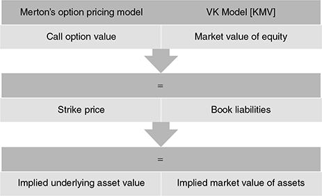
How Merton’s basic options framework is used in the VK Model of KMV is shown in Figure 9.7.
FIGURE 9.7 RELATING MERTON’S MODEL WITh KMV
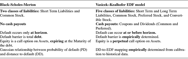
How the Black–Scholes–Merton model differs from the VK model is shown in Table 9.953:
TABLE 9.9 KEY DIFFERENCES BETWEEN THE BSM AND VK MODELS
MKMV combines market value of assets, asset volatility and default point term structure to calculate a DD term structure, which is then translated into a credit measure termed ‘expected default frequency’ (EDF). The EDF is the PD for the risk horizon (1 year or more for publicly traded firms)—and ‘default’ is defined by MKMV as the non-payment of any scheduled payment, interest or principal.
While the core methodology of the EDF model has remained consistent over the years,the model has undergone considerable version updates. The current version is 8.0. Table 9.10 shows the differences between the basic structural model described above and the public EDF model (simply, the EDF model) in its current version.
The public EDF model incorporates the two classic drivers of fundamental credit analysis as we have seen in earlier chapters. Financial risk, or leverage is measured in terms of the difference between the market value of assets and the book value of liabilities, and business risk,is measured by asset volatility—the higher the volatility, the higher the business risk. In addition, the EDF model framework allows for a clear understanding of the consequences of changes in these two primary drivers on a firm’s default risk.
TABLE 9.10 KEY DIFFERENCES BETWEEN THE BASIC STRUCTURAL MODEL (BSM MODEL) AND THE CURRENT VERSION OF THE EDF MODEL

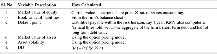
The procedure adopted by MKMV54 for calculating the PD of a public firm can be described in the following three steps:
- Estimate asset value and volatility from the market value and the volatility of equity and the book value of liabilities. This is done using the option nature of equity, as given in the Merton model in Box 9.4 The Market value of equity is observed and the market value of the firm (assets) is derived from it. The model solves the following two relationships55 simultaneously:
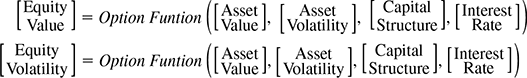
The model solves for ‘asset value’ and ‘asset volatility’ based on the observed inputs of equity value and volatility and the capital structure. The ‘interest rate’ used in this model would be the ‘risk-free’ rate (option pricing theory).
- Calculate the DD as = (market value of assets – default point)/(market value of assets × asset volatility) The numerator reinforces the fact that if the market value of assets falls below the default point, the firm defaults. Hence, the PD is the probability that this event happens.
If the future distribution of the DD were known (over the relevant risk horizon), the default probability—called the expected default frequency (EDF)—would be the likelihood of the final asset value falling below the default point.
In practice, however, it is difficult to accurately measure the DD distribution. MKMV uses the fact that defaults occur either due to large adverse changes in market value of assets or changes in the firm’s leverage, or a correlation of these two factors, and measures DD as the number of standard deviations the asset value is away from default, and then uses empirical data to determine the corresponding PD.
This process is pictorially depicted in MKMV documents56 in figure 9.8.
- The current asset value.
- The distribution of the asset value at time H.
- The volatility of the future assets value at time H.
- The level of the default point, the book value of the liabilities.
- The expected rate of growth in the asset value over the horizon.
- The length of the horizon, H.
- Calculate the default probability
As stated in the earlier paragraph, default probability is empirically determined from data on historical default and bankruptcy frequencies.
Summarizing, the calculations for EDF are done in Table 9.11 using the relevant variables shown in step 2:
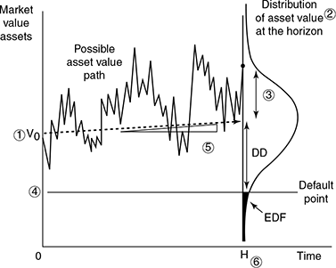
TABLE 9.11 CALCULATIONS FOR EDF USING THE RELEVANT VARIABLES
The final step is to map the DD to actual probabilities of default over the determined risk horizon. These are the EDFs, which are calculated from a large sample of firms including those that defaulted. Based on this historical information, the model estimates, for each time horizon, the proportion of firms with say DD = 4 that actually defaulted after, say, 1 year. If this proportion were, say, 0.33 per cent,57 it is taken to be the EDF of 33 bps. This PD is then assigned an implied rating by the model.
Improvements Made to the Basic Structural Model in the Current Version EDF8.058
While the steps to calculating the PD remain as given above in the basic version, the current version has made improvements in the process to reflect a more realistic estimate of credit risk. The improvements are summarized below:
- Definition of default:
- The basic structural models defined ‘default’ as the ‘non payment of any scheduled payment, interest or principal. However, this is a static definition of default. In practice, identifying events of default can be challenging, and defaults vary in severity across different types of credit events. The range of credit events covered by the default definition would therefore have a direct impact on the credit risk model’s estimation capability.
- In the current version of the EDF model, the range of credit events are considered defaults are (a) missed payments, (b) bankruptcy (as defined by local law), administration, receivership, or legal equivalent, (c) distressed debt restructuring, and (d) government bailoouts enacted to prevent a credit event.
- Estimation of asset value and volatility from equity value and volatility:
- The basic structural model assumes a simplistic relationship between equity volatility and asset volatility.
- However, in practice, it was observed that application of the assumptions of the basic model showed asset volatility estimates to be much greater than actual empirical observations. Since unrealistic asset volatilities would distort PD estimates as well, a number of restrictive assumptions used by the basic model were relaxed, as depicted in Table 9.10 (showing the key differences between the current approach and the basic approach).
- For example, the unrealistic assumption that default can occur only at maturity was replaced by the assumption that default can occur at any time before maturity. While this assumption substantially increased the complexity of the theoretical relationship relating equity and asset values, it led to improvement in the model’s ability to identify default risk. Similarly, the existence of several classes of liabilities was modelled, as well as the possibility of cash leakage over time in the form of dividend payments, coupons on bonds or interest on loans.
- The current EDF model employs a proprietary numerical procedure to incorporate both firm specific asset return information (for empirical volatility estimation), and information from comparable firms (for mod elled volatility estimation). The two volatility estimates are combined to produce the total asset volatility measure used in the current version of the model. An iterative process is followed. Once the asset volatility is estimated and validated, the asset return equation in the basic model serves as the basis for obtaining asset returns. A detailed description of the methodology followed can be found in the quoted paper on the Moody’s Analytics website, www.moodysanalytics.com
- Calculating the Default Point:
- In the basic structural model, the determination of the default point is straightforward—it is simply the face value of a zero-coupon bond (assumed to be the only liability of the firm) whose maturity is the same as the default horizon.
- In practice, firms’ liabilities are often comprised of multiple classes of debt with various maturities. This also means that the same amount of total liabilities for two otherwise identical firms may have different required debt payments for a given time horizon. So the default point is a function of both the prediction horizon and the maturity structure of liabilities. Further, the default point is dependent on the definition of default (see point 1 above). Additionally, there are balance sheet items that are included in a firm’s stated liabilities, but that do not have the potential to force it into bankruptcy. Examples include deferred taxes and minority interests. Estimating default point realistically leads to the realistic estimation of the Distance to Default (DD), which in turn, maps to the PD estimation.
- The current version of the model therefore attempted empirical methods to reconcile the practical issues. In practice, it was observed that large firms do not always default when their asset values fall below their liability values, since they managed to survive through alternate sources of funding. In other cases, observations showed that some firms defaulted even when they could not service their short term liabilities. Hence the model proposed two algorithms—one for financial firms and the other for non financial firms.
- For nonfinancial firms, the default point for a one-year time horizon is set at 100 per cent of short-term liabilities plus one-half of long-term liabilities (as in the earlier version).
- For financial firms, it is more difficult to differentiate between long-term and short-term liabilities. As a consequence, the approach used in the EDF model is to specify the default point as a percent of total adjusted liabilities. This percentage differs by subsector (e.g., commercial banks, investment banks, and non-bank financial institutions).
- Distance to default:
As in the basic structural model given above, DD is calculated as = [Market value of assets – Default point]/ [Market value of assets × asset volatility]
- DD to EDF mapping:
- The EDF model constructs the DD to PD mapping based on the empirical relationship (relationship evidenced by historical data) between DDs and observed default rates. The default database is maintained by Moody’s Analytics.
- The process for converting DD to EDF begins with the construction of a calibration sample (of large sample of corporate firms), and then grouping the sample into buckets according to firms’ DD levels and fitting a nonlinear function to the relationship between DDs and observed default frequencies for each bucket. The EDF model produces not just a one-year horizon EDF for each firm, but also a term structure of EDF measures at horizons of up to ten years.
- An additional feature of the current version of the model is that it accommodates the existence of ‘jumps-to-default’. These are changes in asset values during a short time window, or due to unexpected events, such as corporate fraud or collapse of the business environment.
- EDF Measures:
EDF metrics range from 1 basis point to 35 per cent. The interpretation of EDF measures is as given earlier.
- EDF term structures:
Default probabilities over a longer period in time are necessary for pricing, hedging and risk management of long term obligations. In particular, portfolio models of credit risk, such as Moody’s Analytics’ Risk Frontier platform, require term structures of PDs as key inputs for the valuation of long-dated credit portfolios. The EDF model described above produces not just a one-year horizon EDF for each firm, but also a term structure of EDF measures at horizons of up to ten years. To build the EDF term structure, the starting point is the DD term structure. Instead of calibrating a separate DD-to-EDF mapping for each time horizon, the EDF model employs a credit migration based approach to build the EDF term structure. The DD transition function is evolved using empirical procedures.
- Model extensions: Over the past two years three new EDF variants have been introduced to help manage differing risk variants, namely, CDS-implied EDFs, Through-the-Cycle EDFs, and Stressed EDFs. Brief descriptions of the methodologies behind these metrics are provided in Appendix A of the cited paper on Moody’s Analytics website. Moody’s Analytics also produces EDFs for private firms, i.e., for entities without traded equity. These are delivered via the RiskCalc platform. Public EDFs (described in detail above) is also delivered on a variety of platforms—web platform, CreditEdge®, and through a daily Data File Service (DFS), an XML interface, and an Excel add-in is also being proposed.
What do the EDF measures indicate?
- EDF measures are not credit scores. They are actual probabilities.
- If a firm has a current EDF credit measure of 3 per cent, it implies that there is a 3 per cent probability of the firm defaulting over the next 12 months.
- That is, out of 100 firms with an EDF of 3 per cent, we can expect, on an average, three firms to default over the next 12 months.
- Further, a firm with 3 per cent EDF measure is 10 times more likely to default than a firm with 0.3 per cent EDF measure.
The above model is suitable for a publicly listed firm, where market value of equity would be readily available to estimate asset prices. If the firm is a private firm, whose market value of equity is not readily available, KMV’s private firm model requires the following additional steps to precede estimation of the firm’s DD:
Step 1 Calculate the Earnings before interest, taxes, depreciation and amortization (EBITDA) for the private firm P in industry I.
Step 2 Divide the industry average market value of equity by the average industry EBITDA. This yields the average ‘equity multiple’ for the industry.
Step 3 Multiply the average industry equity multiple from Step 2 by the private firm’s EBITDA. This gives an estimate of the private firm’s market value of equity.
Step 4 The private firm’s asset value can now be calculated as the market value of equity (Step 3) + the firm’s book value of debt.
From this point onwards, the calculation of EDF can proceed as for a public firm.
In 2015, Moody's Analytics introduced EDF9, the ninth generation of its Public Firm EDF (Expected Default Frequency) model. Although the theoretical basis of the methodology remains the same, several enhancements were introduced in EDF9 that resulted in improved accuracy, stability, and transparency.59
SECTION IV
SELECT APPROACHES AND MODELS— THE ACTUARIAL APPROACH
Credit Risk+™ Model
This model follows the typical insurance mathematics approach, which is why it is called the ‘actuarial model’.
The insurance industry widely applies mathematical techniques to model ‘sudden’ events of default by the insured. This approach contrasts with the prevalent mathematical techniques used in financial modelling, which is typically concerned with modelling continuous price changes rather than ‘sudden events’.
How does the actuarial model differ from other models outlined above—say, the Credit Metrics model, based on the credit migration approach?
In the credit migration approach, credit events (such as default or downgrade) are driven by movements in unobserved ‘latent variables’, which in turn give rise to ‘risk factors’. In a credit portfolio, correlations in credit events occur since different borrowers/counter parties depend on the same risk factors. In the actuarial approach, on the other hand, it is assumed that each borrower has a ‘default probability’, but no latent variables. This PD changes in response to macroeconomic factors. If two borrowers are sensitive to the same set of macroeconomic factors, their default probabilities change together, which in turn, give rise to ‘default correlations’.
Credit Risk1 has been developed based on the actuarial approach (insurance modelling techniques) by Credit Suisse Financial Products (CSFP).60 In this model, only default risk is modelled, not downgrade risk. The model makes no assumptions about the causes of default. Each borrower/counter party can assume only one of two ‘states’ at the end of the risk horizon, say, 1 year— ‘default’ (0) or ‘no default (1). The basic model setting is outlined in Box 9.5.
BOX 9.5 THE BASIC MODEL SETTING OF THE ACTUARIAL APPROACH IN CREDIT RISK+
- Assume a portfolio of N borrowers where n = 1,…, N, where the exposure to borrower n is E and the PD of borrower n is pn.
- Default of borrower n is represented by a ‘Bernoulli’61 random variable Dn such that at the end of the risk horizon, say, 1 year, the PD P(Dn = 1) = pn and the probability of ‘survival’ (no default) P(Dn = 0) = 1 – pn .
- If En is the exposure of the bank to borrower n, the total loss of the portfolio at the end of the year is given by

- The objective is to determine the probability distribution of L under various sets of assumptions. Knowing the probability distribution of L will enable computing VaR and other risk measures for this portfolio.
- There are two assumptions made under this model :
- For a loan or borrower or counter party, the PD during 1 year (the risk horizon) is the same as the PD for any other year; and
- Given a large number of borrowers/counter parties, the PD of any one borrower is small, and the number of defalts that occur during any 1 year is independent of the number of defaults that occur during (N ) any other year.
- The probability distribution for the number of defaults during 1 year is then modelled as a Poisson distribution.62 The probability of realizing n default events in the portfolio in 1 year is given by the expression 63
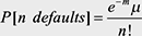
where n = 0,1,2,…, is a stochastic variable with mean µ and standard deviation√µ
µ = average [expected] number of defaults per year. For example, if µ = 4, over the next one 1 year,

And

- It can be noted from the above equation that the distribution has only one parameter, µ. The distribution does not depend on the number of exposures in the portfolio, or the individual probabilities of default, provided these probabilities are uniformly small.
Credit Risk + models credit risk in two stages as shown in Figure 9.10. This approach is typically used in evaluating losses originated in insurance portfolios. The cumulative average EL is arrived at using the loss frequency average and the loss severity average. However, for a dynamic analysis of risks, it is necessary to quantify loss variability by computing the distribution of cumulative losses that would combine the effects of frequency and severity of losses.
Applied to a credit portfolio, the concepts are understood as follows:
- Frequency—the number of defaults in a portfolio over the risk horizon (typically 1 year), and
- Severity—the amount, in currency units, of each individual default, that is, the LGD.
FIGURE 9.10 CREDIT RISK + STAGES IN MODELLING CREDIT RISK

We will describe these processes briefly.
Stage 1
- Frequency of defaults: There are two important inputs to estimate the frequency of defaults—the aver age (expected) default rates, and the volatility (standard deviation) of defaults. Since we have assumed that a standard Poisson distribution can be used to estimate the distribution of the number of defaults, it follows that the volatility (standard deviation) of the number of defaults would approximate to √µ, where µ is the expected (average) default rate. However, this may not hold true in practice, since the default volatility changes over time, depending on business cycles and other factors, and the expected default rate would also change over time. In such a case, would the Poisson distribution still represent the default process? Yes, if we assume that the mean default rate is ‘stochastic’ with mean μ and standard deviation σ and that the mean default rate is ‘gamma distributed’. (Please see our discussion on the KMV model for a brief definition of a gamma distribution).
- Severity of the losses: This is given by the ‘LGD’—the ‘exposure’ of the bank to the borrower, adjusted by the anticipated ‘RR’.
- Distribution of default losses for a portfolio: The model calculates the loss distribution under two scenarios, as shown in Figure 9.11.
FIGURE 9.11 LOSS DISTRIBUTIONS GENERATED BY CREDIT RISK+64
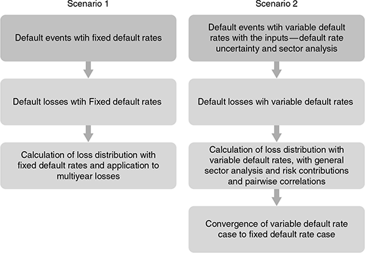
Box 9.6 summarizes the process and notations used by the model in arriving at the loss distributions.
BOX 9.6 PROCESS AND NOTATIONS USED IN CREDIT RISK+
Default losses with fixed default rates
Step 1 Slotting exposures into independent ‘bands’
| Reference | Symbol |
|---|---|
| Obligor/borrower | A |
| Exposure | LA |
| PD | PA |
| Expected loss | λA |
L is chosen as the base currency unit (e.g., ₹in lakh, $1,00,000, etc.), such that for every borrower,
Where vA and ɛA are the exposure and EL, respectively, of the borrower.
Each exposure vA is then rounded off to the nearest whole number.
Thus, the portfolio gets divided into ‘m’ exposure bands, with 1 ≤ j ≤ m.
Step 2 Calculating the expected number of defaults in each band
The following additional definitions are made:
| Reference | Symbol |
|---|---|
| Portfolio exposure in band j in units of L | vj |
| EL in band j in units of L | ɛj |
| Expected number of defaults (mean) in band j | µ j |
The above implies that
If µ is the total expected number of default events in a portfolio in 1 year (the risk horizon), then µ should be the sum of expected number of default events in each exposure band. That is,
Step 3 To derive the loss distribution, calculate the Probability Generating function65 (PGF) for each band, and then for the portfolio.
Step 3A Calculate the PGF for each band, j. This is done using equation (2) of the Credit Risk + technical document (Appendix A, page 34), where the PGF is defined in terms of an auxiliary variable z by66
Since the probability of n defaults is assumed to be a Poisson distribution, we can substitute this with the expression in item 6, Box 9.6. Hence,
Step 3B Calculate the PGF for the entire portfolio. Since each band j is assumed to be a portfolio of exposures, independent from the other bands, the PGF of the entire portfolio is just a product of the PGFs of each band.
Step 3C Calculate the Loss distribution of the entire portfolio. The Credit Risk+ document (equation 25, page 38) derives the following formula:
![]() where An is the probability of loss of ‘n’ units of the portfolio. It should be noted here that the calculation depends only on knowledge of ɛ and v.
where An is the probability of loss of ‘n’ units of the portfolio. It should be noted here that the calculation depends only on knowledge of ɛ and v.
The above initial model, in which loss distribution has been calculated over a 1 year horizon, can be extended to multi-year periods by building a term structure of default for the portfolio. To achieve this, marginal rates of default must be specified for each future year in the portfolio, for each borrower. It can be seen from the
Credit Risk + document (Equations 36, 37, page 40) that the PGF and the loss distribution have the same form as in the single year model described here.
Scenario 2
This scenario assumes variable default rates. The variability in default rates is assumed to result from ‘background factors’, each representing a sector of activity. The sectors are assumed to be independent. To arrive at the loss distribution in such cases, a ‘Mixed Poisson’ process is used.
Simply stated, the ‘Mixed Poisson’ is a two stage process—in the first stage, the external factor controlling the default is drawn from a ‘gamma’ distribution function, and in the second stage, the severity of this external factor is obtained from a conditional distribution that is assumed to be Poisson distributed. The ‘Mixed Poisson’ process is also called a ‘Negative Binomial’ distribution with µ and σ as its mean and standard deviation, respectively.
The ‘gamma distribution’ is a skew distribution that approximates to the Normal distribution when the mean is large. This continuous probability distribution that has two parameters—a scale and a shape parameter—called α and β. It is fully described by its mean µ and standard deviation σ such that µ = αβ and σ2 = αβ2. Hence, for every sector ‘k’, the parameters of the related gamma distribution are given by
In this scenario, the portfolio is divided into n sectors with annual mean default rates following a gamma distribution defined by α and β as defined above. The PGF for each sector is given by the equation:
This can be summed up to the PGF for n sectors, as in Equation 59 (in page 46) of the Credit Risk + document.
The loss distribution is then obtained as described in the Credit Risk + technical document, Section A10.
A simple numerical example in Illustration 9.3 explains the calculation of loss distribution under Scenario 1.
ILLUSTRATION 9.3 CALCULATING THE LOSS DISTRIBUTION WITH FIXED DEFAULT RATES
A bank holds a portfolio of loans with 1000 different borrowers.
For simplicity, we will assume that the exposures fall between ₹50,000 and ₹10 lakh.
Scenario 1
Default Losses with Fixed Default Rates.
Step 1 Slotting Loans into Independent Bands.
We will consider, below, the first six borrowers.
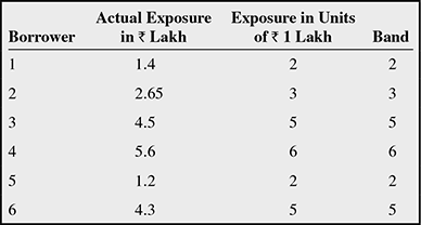
Step 2 Calculating the Expected Number of Defaults in Each Band.
Borrowers in each band are aggregated.
In Credit Risk + each band is viewed as an independent portfolio of loans.
Consider the hypothetical grouping of borrowers in various bands.
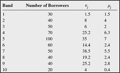
The loss distributions are then modelled using steps 3A, 3B and 3C outlined above.
Appendix B of the Credit Risk + document (1997) provides an illustrative spreadsheet-based example.
SECTION V
SELECT APPROACHES AND MODELS—THE REDUCED FORM APPROACH
We have seen in the foregoing sections that two distinct classes of credit models exist—structural and reduced form.
The structural models discussed in the earlier sections focus on the borrower’s/firm’s fundamental financial variables—assets and liabilities—and link these to the PD. Since we assume complete knowledge of information related to the financial variables (from the firm’s balance sheet), given the firm’s capital structure, and having specified the stochastic process that drives the firm’s asset value (assuming that the market value of the firm is the fundamental source of uncertainty that drives credit risk), the PD for any time horizon (1 year, 2 years, etc.) can be calculated. This implies that a firm’s time of default is predictable. Further, Merton’s model predicts default by allowing a gradual diffusion of asset values to the ‘default point’—the level of debt (see Section III—the KMV model). Such a process would imply that the PD becomes almost zero as the debt approaches maturity—an assumption that may not be true in the real world.
In contrast, ‘reduced-form’ models assume ‘default’ to be an unexpected, sudden event (hence, unpredictable or inaccessible), and assume no explicit relationship between default and firm value. The models basically use the market prices of the firm’s default-prone instruments, such as bonds or credit default swaps (CDS) to extract default probabilities. Thus they rely solely on market information to determine the firm’s credit risk structure, which is much less detailed or complete (compared to the information available from the firm’s financial statements). Since there is no observable link between the firm’s credit risk and its financial situation, the firm’s default time becomes ‘inaccessible’.
The key difference therefore, between structural and reduced-form models, is in the ‘information’ available to model credit risk. While ‘defaults’ are specified ‘endogenously’ (the credit quality being determined by the assets and liabilities of the firm) in structural models, defaults are modelled exogenously from market data in the reduced-form approach. Another difference is in the treatment of RRs—structural models specify RRs based on the value of assets and liabilities within the firm, while reduced-form models look to the market to specify RRs.
Reduced-form models are also called ‘intensity’ models since the input for the models is the intensity of the random time of default within the risk horizon being considered. In practice, the ‘intensity’ of default can be inferred through observed prices of bonds. ‘Default time’ is assumed such that default occurs in a time interval (0, T), where T is the risk horizon (as assumed in the structural models in the previous sections). The default time is driven by an intensity process that is stochastic in nature. These intensity processes define default events, or more generally, credit transitions (as in the structural models), but are directly calibrated to market prices. Though the terms ‘reduced form’ and ‘intensity’ models are used interchangeably, they are in fact two approaches based on the type of information required.
Reduced-form models go back to Artzner and Delbaen (1995),67 Jarrow and Turnbull (1995)68 and Duffie and Singleton (1999).69 The earliest models dealt with just two credit states—default and no-default. Subsequently, various researchers extended the approach to the case of multiple, discrete credit states or ratings, leading to ‘ratings-based’ reduced-form models. The model was further extended to allow for stochastic credit ‘spreads’ (the indicator of credit risk), which were assumed to arise when the underlying default probabilities (intensities) and/or the RRs were stochastic. The theory underlying intensity models is mathematically complex, and will not be explained in this section.70
However, Box 9.7 sets out the basic mathematical premises on which the reduced-form approaches work.
BOX 9.7 BASIC MATHEMATICAL PREMISES OF REDUCED-FORM MODELS
There is no model definition of default in the reduced-form approach. If t, the random default time lies in the time interval (0, T), where T is the risk horizon, in the simplest case, the default process ![]() This is called a ‘point process’ with one ‘jump’ of size ‘1’ at default. (Contrast this with the Merton structural model where there is a gradual fall—’diffusion’—in asset values to the ‘default point’—the debt level).
This is called a ‘point process’ with one ‘jump’ of size ‘1’ at default. (Contrast this with the Merton structural model where there is a gradual fall—’diffusion’—in asset values to the ‘default point’—the debt level).
Typically, reduced-form models characterize default as a Poisson process stopping at the ‘first jump’. The corresponding ‘default time’—called ‘stopping time’—is usually totally unpredictable (‘inaccessible’) implying non-zero credit ‘spreads’ for short maturity debt. Defaults are assumed to occur randomly with a probability determined by the ‘intensity’ or ‘hazard’ function. From this viewpoint, the intensity model can be considered a time continuous extension of the actu arial framework embodied by Credit Risk1 introduced in the previous section.
The model works by decomposing observed ‘credit spreads’ on ‘risky’ debt (debt prone to default) to ascertain the PD and the LGD. This PD is a cumulative, conditional probability—conditional on there being no default before time t. Hence the observed credit spread can be expressed as follows:
where CS is the credit spread (calculated as the risky debt yield minus the risk-free rate),
PD is the probability of default, and
LGD is the Loss given default equal to 1—RR.
Intensity models, therefore, are basically empirical, since they use observable prices of risky debt (and therefore credit spreads).
The differences in the various reduced-form models arise from the assumptions made for calculating PD and LGD. In one of the earliest forms of the approach, Jarrow and Turnbull (1995) infer that the EL over a time period t would be the product of the conditional PD and the RR under the equivalent martingale (the risk neutral measure).71 They assumed that the RR was a known fraction of the value at maturity of the debt. The other well known paper by Duffie and Singleton (1998) assumed that the RR was a known fraction of the value of debt just prior to default, while in their 1999 paper they modelled both PD and LGD as a function of economic state variables. Madan and Unal (1998)72 and Unal et al. (2001) model different RRs on senior and junior debt.
The model developed by Jarrow, Lando and Turnbull in 199773 incorporates probabilities of rating transitions into the process. This can be viewed as a special case of the credit migration approach described earlier.
Kamakura Risk Manager Version 8.0 and Kamakura Public Firm Models Version 5.074
Founded in 1990, with Dr. Robert Jarrow (who pioneered the reduced-form approach) as its Managing Director of Research, Kamakura Corporation (headquartered in Honolulu, Hawaii), provides daily default probabilities and default correlations for listed companies, as well as pricing services for collateralized debt obligations (CDO). The service is called KRIS—Kamakura Risk Information Services.
Kamakura’s Public Firm Models currently offer four different quantitative approaches to modelling default probabilities: two versions of the Jarrow–Chava Model75 (current version 5), the Merton Structural Model and the Jarrow—Merton Hybrid Model
A Brief Description of the Approaches Follows76
The Jarrow Chava Model
The Jarrow Chava Model is a statistical hazard model that relates the probability of firm default to several explanatory variables that include firm financial ratios, other firm attributes, industry classification, interest rates and information about firm and market equity price levels and behavior. In this model, firm default can occur randomly at any time with an intensity determined by the explanatory variables. The model was originally developed by Kamakura’s Director of Research, Robert Jarrow. Both the fourth and fifth generation Jarrow-Chava models incorporate multiple equations for forecasting default at different forward time intervals, conditional on survival to that point in time.The current and forward conditional default probabilities are combined to derive the full default term structure out to five years.
Merton Structural Model
We have learnt in Section II of this chapter about The Merton Structural Model that uses option pricing methods to relate the probability of firm default to its financial structure and information about the firm’s market price of equity.
Jarrow Merton Hybrid Model
The Jarrow Merton Hybrid Model is a statistical hazard model that relates the probability of firm default to the same explanatory variables as the Jarrow Chava Model, but it also incorporates the default probability of the Merton Structural Model as an additional explanatory variable. In this model, firm default can occur randomly at any time with an intensity determined by the explanatory variables.
Which Model is Better—Structured or Reduced Form?
Specific inputs required for structural models
- Firm’s asset value process
- Firm’s capital structure
- LGD
- Terms and conditions of debt issue
Specific inputs required for reduced-form models
- Firm’s default process (bankruptcy process)
- LGD specified as a stochastic process
Common inputs required for both models
- Risk-free interest rate process
- Correlation between risk-free interest rates and asset prices
Thus it can be seen that the solutions/inferences from the models depend on the assumptions, restrictions and different techniques for calibration and solution.
It has, therefore, been claimed by Jarrow and Protter (2004)77 that these models are not disconnected or disjoint model types as is typically assumed. The two types of models, in fact, are really the same model containing different informational assumptions. If information available to the modeller/bank is partial or incomplete, a structural model with default being a predictable ‘stopping time’ becomes a reduced-form model with default time being unpredictable.
To explain the concept further, we know from the Merton’s model that default occurs when the value of the firm falls below a threshold level L. Once the firm defaults, it is assumed that it cannot recover. If we assume that the default barrier is constant (though it can be stochastic), then default occurs at time t, the stopping time, which is predictable. However, in reality, the firm value cannot be monitored continuously, nor is the value observable. Hence, information is not ‘complete’. Even assuming we are able to observe asset values at discrete intervals, there is a likelihood of default occurring between two observations, quite unexpectedly. This implies that the predictable default time t has now become unpredictable. Therefore, the structural model, due to lack of partial information, has taken the form of an intensity-based, reduced-form model.
Hence, the purpose for which the model is to be used determines which model is more appropriate. Jarrow and Protter sum up thus: ‘If one is using the model for risk management purposes—pricing and hedging—then the reduced-form perspective is the correct one to take.
Prices are determined by the market, and the market equilibrates based on the information that it has available to make its decisions. In mark-to-market (MTM) or judging market risk, reduced-form models are the preferred modelling methodology. Instead, if one represents the management within a firm, judging its own firm’s default risk for capital considerations, then a structural model may be preferred. However, this is not the approach one wants to take for pricing a firm’s risky debt or related credit derivatives’.78
SECTION VI
PRICING CREDIT DERIVATIVES
The previous chapter introduced some types of credit derivatives. Though there are several types, credit derivatives typically fall into three discernible classes, and structuring more complex derivatives can be achieved through a combination of the basic features.
FIGURE 9.12 MAJOR CLASSES OF CREDIT DERIVATIVES

However, we have seen that the most popular is the CDS. We will therefore understand the pricing of CDS, an ‘unfunded’ credit derivative that works more like an insurance contract.
Pricing Credit Default Swaps—Understanding the Cash Flows
Understanding the valuation of a single entity (plain vanilla) CDS would provide insights into valuing variations of the CDS, such as binary CDS (where the payoff in the event of default is a specific amount), basket CDS (where more than one reference asset is specified, and the payoff happens when the first reference asset defaults), contingent CDS (where the payoff specifies a credit event as well as an additional trigger) or dynamic CDS (where the notional payoff is linked to a MTM value of a swap portfolio).
It is also important to understand CDS since it is a ‘pure’ credit risk derivative—default probabilities can be ‘extracted’ directly from default swap prices (credit spreads), which can then be used in pricing other credit riskbearing instruments. Hence, CDS can be traded securities79 as well as risk management tools. In our context, we are interested in valuing CDS as a credit risk management methodology.
Several formulas, using different approaches, have been developed for pricing or valuing CDS. However, the default probabilities that they yield are quite comparable, and the various pricing formulas are actually equivalent.80
Let us recap the basics of a single entity CDS.
A CDS is a contract that provides a lender or bank with ‘insurance’ against the risk of default by a specific borrower, firm or counter party. The borrower is called the ‘reference entity’. The default is the ‘credit event’.81 If the credit event occurs, the bank, called the ‘protection buyer’, has the ‘right’ to sell the loan against whose default risk the insurance has been bought. The specific loan whose default risk is being protected against is called the ‘reference obligation’ or ‘reference asset’, and the total value of the loan for which the insurance contract has been created is called the ‘notional principal’.
The cash flows in a CDS occur in two ‘legs’. The ‘protection seller’ provides insurance against default risk. In return, the protection buyer makes a stream of periodical payments (usually quarterly, though semi-annual and annual payments can also happen), until the end of the CDS contract or till a credit event occurs. This is called the ‘premium leg’ (Figure 9.13). The size of these periodic payments are determined from quoted ‘default swap spreads’ to be paid on the notional principal on which default protection is sought.
Default swap spreads, (often simply called ‘spreads’, or sometimes referred to as ‘credit swap premium’,) are quoted in ‘basis points per annum’82 (bpa or bps) on the contracts’ notional principal value. Another point to note that these ‘spreads’ are not the same concept as ‘yield spread’ of corporate bonds to government bonds, and not based on any risk free or benchmark interest rate.83 Several large banks and other institutions are market makers in the CDS market. For example, when quoting on a 5-year CDS on firm F, a bank may ‘bid’ 250 bps and ‘offer’ 260 bps. This is called the ‘bidoffer’ spread and is the typical manner in which quotes are made. This means the bank is willing to ‘buy’ protection on F by paying 250 bps per year (or 2.5 per cent of the notional principal) and ‘sell’ protection at 260 bps per year (2.6 per cent of notional principal). This implies that if Bank A wanted to buy protection against exposure of ₹1 crore to firm F, it would have to pay 62.5 bps [(250/4) bps] per quarter on ₹1 crore or ₹62,500.
If the credit event does not occur till the maturity of the contract, the protection seller does not pay anything. However, if the credit event occurs before the maturity of the contract, the protection seller has to pay as specified in the contract—the swap is then settled either through cash or physical delivery. This is called the ‘protection leg’ and is shown in Figure 9.13.
FIGURE 9.13 CASH FLOWS IN A SINGLE ENTITY CDS
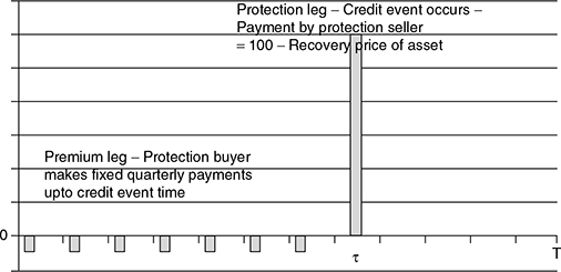
In a CDS settled through cash, the protection seller is required to compensate the loss suffered by the protection buyer by paying the amount of difference between the notional principal and the ‘market price’ of the defaulted bank credit (this approximates to the reduced recovery value). In the case of physical settlement, which is the prevalent market practice, the protection seller buys the defaulted loan from the protection buyer at par. Here the loan purchased by the protection seller is called the ‘deliverable obligation’. The deliverable obligation may be the reference asset itself or one of a broad class of assets meeting certain specifications, usually in respect of seniority and maturity.84 After a credit event, the value of the obligation may be different. Therefore, the protection buyer will deliver the ‘cheapest’ of all deliverable obligations. Hence, this is called the ‘delivery option’. Typically, physical settlement takes place within 30 days of the credit event. Box 9.8 elucidates the ‘cheapest-to-deliver’ concept.
BOX 9.8 THE CHEAPEST-TO-DELIVER CONCEPT
The cheapest–to–deliver bond
The RR of a bond is defined as the value of a bond immediately after default as a percentage of face value. If the CDS is used to hedge the investment in a default prone bond, the payoff from the CDS in the event of default would be (1 – R) × notional principal.
Typically, a CDS specifies that a number of different bonds can be delivered in case of default. These bonds may have the same seniority, but may not be selling at the same proportion of face value immediately after default. This happens because the claim made on default is usually equal to the bond’s face value plus the accrued interest up to default. If a bond has higher accrued interest at the time of default, it tends to have a higher price just after default. Another reason is because the market might feel that there would be differential treatment of bondholders in the event of the firm issuing the bonds being reorganized or restructured. Thus, in the event of default, the protection buyer would tend to choose for delivery the bond that can be purchased most cheaply in the market.
How does the above concept apply to bank loans? Bank A has made a senior, secured loan of ₹100 to borrower firm X and has bought protection through a long CDS position from Bank B. If the credit quality of the loan deteriorates and a credit event is triggered, then the buyer, under physical settlement, delivers the loan now valued at ₹70, down from ₹100 par, to the CDS seller. The seller pays ₹100 to the CDS buyer. Thus, the CDS buyer has made no loss (or profit) on the transaction. On the other hand, the buyer could instead sell the loan at ₹70 (making a loss of ₹30), and buy a junior rank ing bond at, say, ₹50, to deliver to the seller (provided the deliverable obligation permits it). The CDS buyer would still receive ₹100 in settlement, and also make a gain of ₹20 (₹50 gain on CDS less ₹30 loss on loan). Such a practice is useful especially where restructuring is deemed a credit event, since Bank A may not want to sell the asset under restructuring.
In case of cash settlement the protection seller pays the protection buyer an amount equal to the notional principal × (1 – R). Cash settlement is less common since it is difficult to obtain market quotes for the distressed asset. In practice, cash settlement occurs within 5 days after the credit event, and the price will be determined through the Calculation Agent by reference to a poll of price quotations obtained from dealers for the reference obligation on the valuation date.85 The assumption here is that defaulted loans will trade at a price reflecting the market’s estimate of recovery value, irrespective of maturity or interest. In some cases, the cash settlement would be a sum predetermined by the counter parties, which is termed ‘binary settlement’.
Though they seem different, the net value of asset transfer under physical settlement and the net transfer under cash settlement is the same. Under physical settlement, the protection buyer delivers the market value of the deliverable obligation (R × notional principal) and receives in return 100 per cent of the notional principal in cash. The total effect is that of being compensated for the notional principal. Under cash settlement, the asset is with the protection seller and can be realized at R × notional principal. The protection seller merely compensates the loss by paying (1 – R) × notional principal.
Illustration 9.4 clarifies through a numerical example.
Pricing Credit Default Swaps—Grasping the Basics
According to Duffie (1999),86 pricing a CDS involves two issues.
The first issue is estimating the credit swap spread. We have seen in Figure 9.13 that, at the beginning of the contract, the standard credit swap involves no exchange of cash flows and, therefore, has a market value of zero. For convenience, we ignore dealer margins and transaction costs here. The market premium rate, therefore, is that for which the market value of the credit swap is zero.
ILLUSTRATION 9.4 UNDERSTANDING CDS CASH FLOWS
Basic inputs
- Protection buyer, Bank A, wants protection against default risk of firm XYZ.
- The notional principal (face value) on which protection sought for is ₹10 crore. (Bank A may have other exposures to firm XYZ but it wants protection only for ₹10 crore that it considers most vulnerable).
- The protection is required for 2 years (T in Figure 9.13). (Again, the credit limit to firm XYZ may have a maturity period of 5 years, but Bank A needs protection only for the first 2 years).
- The default spread is 300 bps over the risk-free rate (prime rate).
- Bank A has to make quarterly payments to Bank B, the protection seller.
Cash flows
The quarterly payment would amount to 10 crore × 0.03 × 0.25 = ₹ 7,50,000.
Assume that at point τ, (τ < T), the loan to firm XYZ suffers a credit event. At this point, the ‘cheapest to deliver’ (CTD) asset of the firm XYZ has a recovery price of ₹60 per ₹100 of face value.
The cash flows are as follows:
- Bank A, the protection buyer, pays Bank B ₹7.5 lakh per quarter up to the time of the credit event, τ. If the credit event happens, say 1 month after the completion of a quarter, then a proportionate amount (₹7.5 lakh/3 months) of ₹2.5 lakh would be paid.
- Bank B, the protection seller, compensates Bank A for the loss on the face value of the asset, by paying ₹10 crore × (100 per cent – 60 per cent) = ₹4 crore.
The second issue is that, with passage of time, interest rates or credit quality of the reference asset may change, and would impact the market value of the swap. Hence, for a given CDS, with defined periodic payments determined by the credit spread, the current market value would have to be ascertained. This market value would not be zero.
It should be noted that the default probabilities used to value a CDS are ‘risk neutral’ probabilities (and not ‘real world probabilities’).87
The simplest situation is where there is no counter party default risk.88 The other simplifying assumption is that default probabilities, interest rates and RRs are independent. Box 9.9 outlines the basic equations to determine the single entity, CDS credit spread.
BOX 9.9 THE BASIC EQUATIONS TO VALUE A SINGLE ENTITY CDS
Assume Bank A has made a new loan L to firm X, an existing borrower. Bank A wants to transfer the risk of the new loan N (the Notional Principal) to Bank B through a CDS. Bank A is the protection buyer and Bank B, the protection seller. The protection against credit risk is sought for T years (the swap maturity, which need not be the same as the loan maturity). Bank A accepts to pay a fixed fee f for the protection provided by B. For understanding the basics, we will ignore, for the time being, accrued fee amount, if any, at the time of the credit event, and also assume that Bank B has zero PD on its contract with A.
At the time of the credit event (loosely, default), assume the value of the contract to be RN, where R is the already known RR. This means that Bank A would lose (1 – R) × N if it did not buy protection in case of default on the new loan by X. In other words, (1 – R) × N is the payoff of the CDS contract in the event of default. Assuming R as known, the fee f to be paid periodically by Bank A would depend on the market view of the PD by firm X.
Under the contract, Bank A pays f at predetermined periods (e.g., every quarter) until the contract ends at T or until a credit event happens before T. Therefore, the PV of the cash payments by Bank A is the discounted value of each fee pay ment multiplied by the probability that X does not default up to the date of payment.
Assume that CDS premiums (fee payments) are paid on a set of predetermined dates represented by Γ = t1 , t2 ,…, tn . In other words, in a CDS of T maturity starting time 0 (t0 ) and having quarterly payments, the payment dates would be t1 = t0 + 3 (months), t2 = t0 + 3 × 2 months and so on, and tn = T. If p is the PD of X, then p(t1) would be the probability (as seen at time t0) that X will default at time t1. That is, 1 – p(t1)[call it q(t1)] is the probability of no default by X at time t1. If d(t1) is the discount factor pertaining to the prevailing risk-free rate, the expected PV of fee payments by Bank A can be obtained as follows:
The PV of cash flow for Bank B, the protection seller, will be the discounted value of the recovered fraction of N multiplied by the PD at each fee payment date. This implies that for a default occurring at time t(i+1), it is necessary that the firm X has not defaulted up to time ti , and that it defaults exactly at t(i+1). Hence, the weight to be used for calculating expected payment at time t(i+1) is the product of the probability of no default up to ti and the conditional PD between ti and t(i+1). The PV of expected cash flow for Bank B can be represented by the following equation:
However, since default does not occur on a predetermined date, and can occur at any time between ti and t(i+1), we can rewrite the above equation as follows:
Here, the discount factor is the average of the discount factors of the periods within which default may occur, and pti, t i+i is the conditional PD between times i and i + 1, given that default did not occur up to time i.
This implies that the ‘value’ of the CDS to the protection buyer is the difference between the PV of the expected payoff and the PV of payments made by the buyer.
Since we operate under the ‘no arbitrage’89 assumption, the two PVs should be equal at the beginning of the contract. Setting PVf equal to PVrecovery, we can find the CDS rate or fee:
Here, f indicates the CDS ‘spread’. This is an annualized spread.
In practice, CDS spreads are available in the market for different maturities based on the reference asset. We can use the market CDS spreads to arrive at a term structure of default probabilities using the equation above. Assuming we have 1 year, 2 year,…, n year CDS spreads available from the market, we can value the PV of a CDS contract at any point in time using the above equation. For example, if we know that the mid-market CDS spread for a newly issued 5 year CDS is 100 bps, we can work backwards using the above equation and estimate the implied default probability.
One parameter required for valuing a CDS, but cannot be directly observed from the market, is the expected RR. So far, we have assumed the same RR for estimating PD densities, and for calculating the payoff, which means that the estimated CDS spread will not be very sensitive to the RR. This is because the implied probabilities of default are proportional to (1/1–R) and the payoffs from a CDS are proportional to (1–R).
However, the above will not be true in the case of a binary CDS. The payoff in a binary CDS is a fixed amount, regardless of the RR. Since implied probabilities are still proportional to (1/1–R), but the payoff is independent of R, if we have the CDS spread of both a plain (vanilla) CDS and a binary CDS, we can estimate both the RR and the default probability.
The theory implicitly assumes that the reference asset is a floating rate asset, trading at par. However, where such floating rate assets are not available, the market often tries to estimate the CDS spread from a fixed rate asset, trading away from par, using an ‘asset swap’. Asset swaps break down the asset’s yield into a yield (say LIBOR) curve plus a spread. This spread is usually taken as an estimate for the CDS spread.90
Another complication is when the protection seller is prone to default risk.91 In such cases, the CDS spreads reflect the default risk of the seller, or the protection buyers try to get additional/backup protection from the market.
There are other methodologies used to price CDS spreads. The reduced-form models (described in section V) are used extensively for this purpose. The Jarrow–Turnbull (1995)92 model assumes recovery to be a fixed amount in the event of default, and is, therefore, called a ‘fixed recovery model’. In a ‘market standard’ model based on the Jarrow–Turnbull model, O’Kane and Turnbull (2003)93 propose that the PD occurring within the time interval (t, t + dt), conditional on ‘no default’ up to time t, is proportional to a time-dependent function λ (called the ‘hazard rate’), and the length of the time interval dt. Hence, the model uses a simple ‘binomial tree’94 where the probability of no default is 1–λdt, and if there is default the recovery value R is received with probability λdt. This model can be extended to multiple time periods and continuous time probabilities (as compared with discrete time probabilities used in Box 9.9) of default and no default can be arrived at.
The Duffie–Singleton (1999)95 model assumes the amount of recovery is restricted and is, therefore, referred to as the ‘fractional recovery model’.
The CDS market is largely over-the-counter (OTC). This means that the protection buyer and seller negotiate each CDS trade, at the time it is required—hence, each CDS will have a separate reference asset, notional amount, maturity, credit event definition, CDS spread, etc. Once the terms are agreed to by the counter parties, the trade is finalized through proper documentation. Default swaps are looked upon as a good source of expected return for protection sellers.
Credit derivatives are used by different groups of investors for a variety of reasons. Banks are understandably major protection buyers and sellers, in order to mitigate the credit risk in their large loan portfolios. Insurance firms are major protection sellers, who also provide protection against counter party risk for protection buyers.
We will illustrate estimation of CDS spread with a simple numerical example (Illustration 9.5).
ILLUSTRATION 9.5 CALCULATION OF CDS SPREAD—A SIMPLE EXAMPLE
Assumptions:
- The notional principal is 1 (monetary value in any currency, e.g., ₹1 or $1, etc.)
- The PD p of a reference entity is assumed to be 2 per cent at the end of year 1, provided there is no earlier default. This is the conditional PD.96
- The above implies that the probability of no default q at the end of year 1 is 98 per cent.
- The protection buyer seeks protection for 5 years.
Step 1 Construct Table 9.12 of unconditional probabilities of default over 5 years (i.e., PD viewed at time ‘0’)
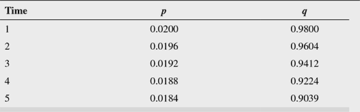
How did we obtain the above probabilities? For year 1, we know that p = 2 per cent and q = 98 per cent. For year 2, p = q of year 1 × p = 0.9800 × 0.02 = 0.0196 and q (year 2) = probability of no default in both years = 0.9800 × 0.9800 = 0.9604. For year 3, p = probability of no default for 2 years (q of year 2) × p =0.9604 × 0.02 = 0.0192 and q = probability of no default for 2 years × q = 0.9604 × 0.9800 = 0.9412 and so on.
Step 2 Calculate the cash flows of the protection buyer, assuming the riskfree rate97 to be 6 per cent per annum. Since payments will be made by the protection buyer only in the case of no default, we take q over 5 years to estimate the expected fee payment. Let the fee to be paid be f.
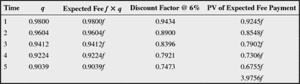
The total expected cash flow of the protection seller over the 5 year CDS would be 3.9756f
Step 3 Cash flow of protection seller in case of credit event
We know that p is the probability of credit event (default) over the life of the CDS. If we assume 50 per cent RR, the protection seller will have to settle 100 – R or 100 – 50 in case of a credit event (see Figure 9.13). We also assume that the credit event is likely to occur only at the end of the year.
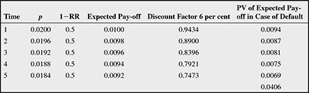
The expected payoff is calculated as p × (1 – RR) for each year. The PV of the expected payoff for the protection seller is seen to be 0.0406.
Step 4 Equate the two PVs in steps 2 and 3 and solve for f.
3.9756f = 0.0406
Hence, f = 0.0102 or 102 bps per year credit spread.
Note that the simple example is given to illustrate the calculation methodology. In practice, there are more complications, such as fee payments by the protection seller may be made quarterly or half yearly, or the credit event may occur at any time during the year. We have also assumed the protection seller will not default in settling the CDS.
Let us now turn to the second issue raised by Duffie (1999) outlined in an earlier paragraph.
At the time it is priced, the CDS, like most other swaps,98 is worth almost nothing. Assume that the protection buyer in the Illustration 9.5 wants to value its position after 1 year. On the date of such revaluation, CDS spreads quoted in the market are 125 bps for a 4-year CDS (the 4-year spread is relevant since the protection was sought for 5 years in the example, and 1 year has since elapsed). What is the current market value of the position?
The MTM value = current market value of remaining 4-year protection less the expected PV of 4-year premium leg at the earlier calculated spread of 102 bps. It is to be noted here that the CDS contract has increased in value since the protection buyer is paying only 102 bps for something the market is now willing to pay 125 bps. Since the MTM of a new CDS is zero, the current market value of remaining 4-year protection becomes equal to the expected PV of the premium leg at 125 bps. It therefore follows that the MTM value to the protection buyer is the difference between the expected PV of 4-year premium leg at 125 bps and the expected PV of 4-year premium leg at 102 bps.
In Illustration 9.5, the expected PV of the protection buyer’s fee payments would change to 3.9756 × 0.0125 = 0.0497. The PV of the payoff (assuming RR is the same) would remain at 0.0406. The market value of the swap would now be 0.0497 – 0.0406 = 0.0091 times the notional principal. In other words, the MTM value of the CDS to the protection buyer would now be –0.0091 times the notional principal.
In case of a binary default swap, the numbers in Illustration 9.5 would change as follows:
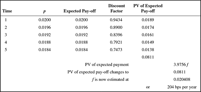
In 2009, ISDA introduced the ISDA CDS standard model, the source code for CDS calculations, as a free download from its Web site, which can be accessed at www.cdsmodel.com