Chapter 5

Sampling and Sampling Distributions

Learning Objectives

Upon completion of this chapter, you will be able to:

• Understand the importance of sampling
• Differentiate between random and non-random sampling
• Understand the concept of sampling and non-sampling errors
• Understand the concept of sampling distribution and the application of central limit theorem
• Understand sampling distribution of sample proportion

5.1 Introduction

While conducting research, a researcher has to collect data from various sources. We have already discussed that for collecting data, relying on the entire population is neither feasible nor practical. So, a researcher has to select a sample instead of going in for a complete census. A researcher faces problems in terms of the procedure of selecting a sample. Statistical inference is based on the information obtained from the sample. On the basis of information obtained from the sample (through sample statistic), an inference about the population (population parameter) is made. In this process, we need to keep in mind that the sample contains only a portion of the population and not the entire population. So, a proper sampling method should be used for selecting a sample. In order to make a good estimate of the population characteristics, selecting a reasonably good sampling method is of paramount importance.

This chapter focuses on the various issues related to sampling and sampling distributions. It also presents the distribution of two very important statistics; sample mean and sample proportion. Sample mean and sample proportion are normally distributed under certain conditions. The knowledge of these statistics form the foundation of statistical analysis and inference.

5.2 Sampling

Sampling is the most widely used tool for gathering important and useful information from the population. A researcher generally takes a small portion of the population for study, which is referred to as sample. The process of selecting a sample from the population is called sampling. As a part of the research process, we collect information from the sample, apply statistical tools and techniques for the analysis, and make important interpretations on the basis of statistical analysis. Decisions are then taken on the basis of this interpretation. For example, there are two methods of determining the degree of job satisfaction of a company having 120,000 employees. The first method is to prepare a well-structured questionnaire and administer it to all employees. This method would be very expensive and cumbersome. The second method is to select a representative sample from the population and make decisions on the basis of the information obtained from the sample (after applying all the necessary statistical tools and techniques). Therefore, census is not a practical method of gathering information in many situations because of the time, costs, and other constraints involved. In other words, we can say that sampling is the only practical solution in certain situations.

5.3 Why is sampling essential?

We have discussed the advantages of sampling over a complete census. The following points reinforce this statement.

• Sampling saves time.
• Sampling saves money.
• When the research process is destructive in nature, sampling minimizes the destruction.
• Sampling broadens the scope of the study in light of the scarcity of resources.
• It has been noticed that sampling provides more accurate results, as compared to census because in sampling, non-sampling errors can be controlled more easily. (The concept of non-sampling errors will be discussed in detail later in this chapter).
• In most cases complete census is not possible and, hence, sampling is the only option left.

5.4 The Sampling Design Process

Sampling design process can be explained by five interrelated steps. These five steps are shown in Figure 5.1.

Figure 5.1 Steps in sampling design process

Step 1: Target population must be defined

The target population should be defined in the light of a research objective. Target population is the collection of objects, which possess the information required by the researcher and about which an inference is to be made. Improper definition of the target population will lead to misleading results which might prove dangerous for a researcher. Therefore, target population must be defined very carefully. As discussed earlier, the research objective should be the most important factor to be taken into account while deciding on the target population. However, other parameters like time and cost should not be ignored.

Step 2: Sampling Frame must be determined

A researcher takes a sample from a population list, directory, map, city directory, or any other source used to represent the population. This list possesses the information about the subjects and is called the sampling frame. It might seem that the target population and the sampling frame are the same, however, in reality, there is a reasonable difference between the two. For understanding this difference, let us take the example of a telephone directory. A telephone directory possesses information about a particular region. When we take a sample on the basis of information available in a directory, there is a possibility that this will not give us true information. It is always possible that few subjects in that region may not have telephones, few subjects may have changed their residence and this information might not have been updated in the telephone directory. Similarly, some subjects may have multiple listings under different names; some subjects may have changed the numbers ever since the directory was printed. Sampling is carried out on the sampling frame and not on the target population. Theoretically, the target population and the sampling frame are the same, however, in practice, sampling frame and target population are often different. Over-registered sampling frames contain all the units of target population plus some additional units. Under-registered sampling frames contain fewer units as compared to the target population. A researcher’s objective is to minimize the differences between the sampling frame and the target population.

Step 3: Appropriate sampling technique must be selected

Selecting a sampling technique is a crucial decision for a researcher. A researcher has to decide between the Bayesian or the traditional sampling approach, sampling with or without replacement, and whether to use probability or non-probability sampling techniques.

The Bayesian approach is theoretically very sound, but practically not very appealing. It is based on prior information about the population parameters. It is very difficult to obtain the required information essential for applying the Bayesian approach. Hence, its use is very limited in research. The traditional approach is more appealing and is widely used. In the traditional approach, the entire sample is selected before data collection begins.

In sampling with replacement, an element is selected from the frame, the required information is obtained, and then the element is placed back in the frame. This way, there is a possibility of the element being selected again in the sample. As compared to this, in sampling without replacement, an element is selected from the frame and not replaced in the frame. This way, the possibility of further inclusion of the element in the sample is eliminated.

The most important part of selecting a sampling technique is making the choice between random sampling and non-random sampling techniques. This is very important and is discussed in detail in this chapter.

Step 4: Sample size must be determined

Sample size refers to the number of elements to be included in the study. While deciding the sample size, various qualitative and quantitative aspects must be considered. In this section, we are going to discuss the qualitative aspects of sample size, while the quantitative aspects will be discussed later. The nature of research and analysis, number of variables, sample size used for similar kind of study, time, resources, incidence rates, and completion rates are some of the qualitative considerations that need to be taken into account when taking a decision about the sample.

The nature of research and analysis is an important consideration while deciding the sample size. For qualitative research, a small sample size is sufficient. For conclusive research, a larger sample is required. Sophisticated statistical analysis is also a foundation for taking a decision about the sample size. The statistical analysis techniques applied for analysing small and large samples are different. In case of multivariate analysis or when the data is being analysed at the subgroup or segment level, large data are required. Similarly, when data are collected for a large number of variables, large samples are required. The cumulative errors across variables are reduced in a large sample.

Sample size used for similar studies can also be used as a basis for selecting sample size. This is more useful when non-probability sampling techniques are used for the study. Time and resources are the two constraints on which the sample size of every research study is based. Sample size should also be adjusted with respect to factors such as eligible respondents and the completion rate.

Step 5: Sampling process must be executed

The execution of sampling techniques requires detailed specification of target population, sampling frame, sampling techniques, and the sample size. At this stage, each step in the sampling process must be effectively executed.

5.5 Random versus Non-random Sampling

Sampling procedure can be broadly divided into two categories: random and non-random sampling. In random sampling, each unit of the population has the same probability (chance) of being selected as part of the sample. In random sampling, the chance factor comes into play in the process of sample selection. For statistical analysis, a random sample is ideal. However, there may be some cases where random sampling is not feasible. In these cases, non-random sampling methods can be good alternatives. As compared to random sampling, in non-random sampling, every unit of the population does not have the same chance of being selected in the sample. In non-random sampling, members of the sample are not selected by chance. Some other factors like familiarity of the researcher with the subject, convenience, etc. are the basis of selection. On the basis of the selection procedure used, random and non-random sampling techniques are referred to as probability and non-probability sampling, respectively. Figure 5.2 depicts the broad classification of random sampling methods and non-random sampling methods.

Figure 5.2 Random and non-random sampling methods

5.6 Random Sampling Methods

We have discussed that in random sampling methods, every unit of the population has an equal chance of being selected in the sample. As shown in Figure 5.2, the random sampling methods used for selecting samples from the population are as follows:

5.6.1 Simple Random Sampling

In simple random sampling, each member of the population has an equal chance of being included in the sample. Simple random sampling is the most common method of selecting a sample from the population. In the simple random sampling method, first, a complete list of all the members of the population is prepared. Each element is identified by a distinct number (say from 1 to N). Then n items are selected from a population of size N, either using random number tables or the random number generator. Random number generator is usually a computer program that generates random numbers. The random number table has been developed by statisticians. For small populations, simple random sampling is appropriate, but when the population is large, simple random sampling becomes cumbersome. This is because numbering all the members of the population and then selecting items is not an easy task.

Simple random sampling is based on the process of selecting a sample randomly. This does not mean that the randomness allows haphazard selection of samples; it means that the process of selecting a sample should be free from human judgement (bias). In this context, there are two methods of drawing a random sample from the population. These two methods are: (1) the lottery method and (2) the use of random numbers.

In the lottery method, each unit of the population is properly numbered. The numbers are written on different pieces of paper. The pieces of paper are then folded and mixed together in a small box. A sample of our choice can be drawn randomly from the box (by selecting folded papers randomly).

The second method to draw a random sample is to use a random number table. The units of the population are numbered from 1 to N. A sample of size n has to be then selected. The following example explains the use of random number tables.

Suppose a researcher wants to conduct a survey related to attitude measurement in five companies. He has a list of 25 companies. He wants to select 5 companies out of 25 through the simple random sampling method. The first step is to number each unit of the population. For this purpose, we select as many digits for each unit sampled, as there are in the largest number in the population. For example, if there are 700 members in a population, we select three-digit numbers like 001, 003, 045, 054 for the first, third, forty-fifth and fifty-fourth units, respectively.

A researcher wants to select five companies out of 25, so in this case, each unit of the population is numbered from 1 to 25 with two-digit numbers, as explained earlier. This population contains only 25 companies, so all the numbers greater than 25, that is, (26–99) must be ignored. For example, if a number 58 is selected, it is ignored and the process is continued until a value between 1 to 25 is obtained. Similarly, if the same number occurs the second time, we proceed to another number. Table 5.3 depicts a part of the random number table.

Table 5.3 A part of the random number table

The researcher’s objective is to select 5 companies out of 25, so different two-digits numbers must be selected from the table of random numbers. For this, we start from the first pair of digits from the random number table and proceed across the first row until we get the required 5 companies in terms of the different values between 01 and 25. Here, we have started the selection of samples from the first row of the random number table, but it may be done from anywhere in the table.

In Table 5.4, a list of 25 companies is given from which the researcher wants to select 5 companies for his study. The list given in Table 5.4 is not numbered and the list is numbered in Table 5.5 for convenience in sample selection.

Table 5.4 A list of 25 companies

From Table 5.3, the first two digit number is 12 which lies between 01 and 25. So, this number can be selected as the first number of choice. The next two numbers are 65 and 16. The number 65 is out of the range of the selection criteria. So, the next two digit number 16 is selected, which is within the range of the selection criteria. In a similar manner, we proceed further and select five two-digit numbers as 12, 16, 11, 09, and 25. In this manner, from Table 5.5, the 12th, 16th, 11th, 09th, and 25th companies are selected in the final sample. So, in this manner the final sample will consist of the following five companies:

Table 5.5 A numbered list of 25 companies

Tata Iron and Steel Company Ltd

Maruti Udyog Ltd

Mahanagar Telephone Nigam Ltd

Larsen & Toubro Ltd

Ranbaxy Laborataries Ltd

5.6.2 Using MS Excel for Random Number Generation

For several probability distributions, random numbers can be generated by MS Excel. For this, select Data from the menu bar and then select Data Analysis. From the Data Analysis dialog box, select Random Number Generation. The required distribution can be selected from the third box of the Random Number Generation dialog box. Select the distribution for which the random numbers are to be generated (Figure 5.3). With the selected distribution, the options and the required responses in the Random ­Number Generation dialog box will change accordingly. In each case, the number of variables should be filled in the first box and the number of random numbers to be generated should be filled in the second box (Figure 5.3).

FIGURE 5.3 MS Excel Random Number Generation dialog box (for normal distribution)

5.6.3 Using Minitab for Random Number Generation

Minitab can also be used for random number generation for various probability distributions. For this purpose, click Calc/Random Data/Normal. The Normal distribution dialog box as shown in Figure 5.4, will appear on the screen. Note that like normal distribution, any of the probability distributions can be used for random number generation. As shown in Figure 5.4, the random numbers to be generated should be placed in the Generate rows of data box. For example, if we want to generate 50 random numbers, we need to place 50 in the box, as shown in Figure 5.4. In Store in column(s) box, place the column location where we want to store the random numbers. The required mean and standard deviation can also be placed in the concerned boxes. Like normal distribution, each distribution requires specific parameters. According to the requirement, these parameters can be placed in the concerned boxes and random numbers for concerned specific probability distributions can be generated.

FIGURE 5.4 Minitab Normal Distribution dialog box (for random number generation)

5.6.4 Stratified Random Sampling

Stratified random sampling is based on the concept of homogeneity and heterogeneity. In stratified random sampling, elements in the population are divided into homogeneous groups called strata. Then, researchers use the simple random sampling method to select a sample from each of the strata. Each group is called stratum. In stratified random sampling, stratum should be relatively homogenous and the strata should contrast with each other. This process of dividing heterogeneous populations into relatively homogenous groups is called stratification. In most cases, researchers use demographic variables as the base of stratification. For example, a company that produces perfume wants to know the consumer preference for its newly launched product. For this purpose, company researchers have to select a sample of 1000 consumers from a particular town with a population of 1,000,000. This population contains people from different age groups, education, regions, religion, etc. These groups may have different reasons for preferring a brand. Taking 1000 people randomly from the population will not lead to an accurate result because they may not be true representatives of the population. So, instead of selecting people directly from the population, we need to divide this heterogeneous population into homogenous groups, and then simple random sampling procedure can be used to obtain the samples from these homogenous groups. A researcher has to keep in mind that within each group, homogeneity or alikeness must be present and between the groups, heterogeneity must be present.

Stratified random sampling can be either proportionate or disproportionate. In cases where the percentage of sample taken from each stratum is proportionate to the actual percentage of the stratum within the whole population, stratified sampling is termed as proportionate stratified sampling. For example, suppose in a population, 75% are matriculates, 15% are graduates, and 10% are postgraduates. A researcher uses the stratified random sampling based on educational level and selects a sample of size 1000. This sample is required to have 750 matriculates, 150 graduates, and 100 postgraduates to achieve proportionate stratified sampling. On the other hand, a sample of 600 matriculates, 200 graduates, and 200 postgraduates will lead to disproportionate stratified random sampling. So, in cases, where the sample taken from each stratum is disproportionate to the actual percentage of the stratum within the whole population, disproportionate stratified random sampling occurs. Figure 5.5 exhibits the stratified random sampling based on educational levels.

Figure 5.5 Stratified random sampling based on educational levels

5.6.5 Cluster (or Area) Sampling

In cluster sampling, we divide the population into non-overlapping areas or clusters. It might seem as there is no difference between stratified sampling and cluster sampling. This is not true; in fact there is a well-defined difference between stratified sampling and cluster sampling. In stratified sampling, strata happen to be homogenous but in cluster sampling, clusters are internally heterogeneous. A cluster contains a wide range of elements that are good representatives of the population. For example, a fast-moving-consumer-goods company wants to launch a new product and wants to conduct a market study. For this, the country can be divided into clusters of cities and then individual consumers within cities can be selected for the survey. In this case, clusters of cities may be too large for surveying individuals. In order to overcome this difficulty, the city can be divided into clusters of blocks and consumers can be selected randomly from the blocks. This technique of dividing the original cluster into a second set of clusters is called two-stage sampling.

Cluster sampling is very useful in terms of cost and convenience. When compared to stratum in stratified random sampling, clusters are easy to obtain and focus of the study remains on the cluster instead of the entire population, so cost is also reduced in cluster sampling (Figure 5.6). In real life, cluster sampling becomes the only available option because of the unavailability of the sample frame. This does not mean cluster sampling is free from drawbacks. Cluster sampling may be statistically inefficient, in cases where elements of the cluster are similar.

Figure 5.6 Diagram for cluster sampling

5.6.6 Systematic (or Quasi-Random) Sampling

In systematic sampling, sample elements are selected from the population at uniform intervals in terms of time, order, or space. For obtaining samples in systematic sampling, first of all, a sampling fraction is calculated. For example, a researcher wants to take a sample of size 30 from a population of size 900 and he has decided to use systematic sampling for this purpose. As the first step, he has to calculate a sample fraction k, which is equal to , where N is the total number of units in the population and n is the sample size.

So, in this case, sample fraction will be = 30. For obtaining the sample, the first member can be selected randomly and after that every 30th member of the population is included in the sample. Suppose the first element 3 is selected randomly and after this, every 30th element, that is, 33rd, 63rd, … element up to a sample size of 30 are included in the sample. For obtaining starting point or the beginning point of the sampling process, a random number table can also be used. In our example k = 30, so a researcher can use a random number table to get the first element between 1 and 30.

In systematic sampling, the selection of a sample is very convenient and is cost and time efficient. This is an aspect of systematic sampling which makes it applicable in many situations. However, systematic sampling has certain limitations. In systematic sampling, the first unit is selected randomly and the selection of remaining units is based on the first unit. So, randomness of the selected sample units can be questioned. There can be another problem with systematic sampling; if the data are periodic and the sampling interval is in syncopation with it. For example, consider a list of 250 consumer groups that is a merged list of five income classes with 50 consumers in each class. The list of 50 consumers is an ordered list of consumers with some predefined sequence in data. If a researcher uses systematic sampling, then on the basis of the first selected unit, the possibility of including almost all high-income groups, almost all middle-income groups or lower-income groups in the sample cannot be ignored because the original population is arranged in order. Let us assume that, this researcher wants to take a sample of size 10 from the population of size 250. As discussed the sample fraction will be . The researcher selects the first unit as the 25th item (randomly) and then selects every 25th unit such as 50th, 75th, 100th, …, 250th unit. As there is some predefined sequence in the data, the possibility of selecting all the 10 units or maximum units from a particular income group cannot be ignored. Systematic sampling is based on the assumption that the source of the population element is random. Systematic sampling is some times known as quasi-random sampling.

5.6.7 Multi-Stage Sampling

As the name indicates, multi-stage sampling involves the selection of units in more than one stage. The population consists of primary stage units and each of these primary stage units consists of secondary stage units. In the process of multi-stage sampling, first, a sample is taken from the primary stage units and then a sample is taken from the secondary stage units. For example, a researcher wants to select 200 urban households from the entire country and wants to use multi-stage sampling for this. For this purpose, he may first select 27 states from the country as the primary sampling unit. During the second stage, 50 districts from these 27 states may be selected. Finally, 4 households from each district may be randomly selected. Thus, a researcher will obtain the required 200 urban households in two stages.

Though this type of sampling may be costly, it will be a true representative of the entire population. The number of stages in multi-stage sampling is a matter of the researcher’s discretion. On the basis of convenience or the discretion of the researcher, a few stages can be deleted or included in multi-stage sampling. In the previous example, the last stage was at the district level, which may be expensive and inconvenient. So, to avoid this difficulty, two more stages, in terms of cities and blocks can be included in the sampling process. In this manner, stages of the sampling can be as shown in Figure 5.7.

Figure 5.7 Multi-stage (four stages) sampling

5.7 Non-random Sampling

Sampling techniques where the selection of the sampling units is not based on a random selection process are called non-random sampling techniques. In the selection of the sample units, the probability (of being included in the sample) is not used, which is why these techniques are also termed as non-probability sampling techniques. Quota sampling, convenience sampling, judgement sampling, and snowball sampling techniques are some of the commonly used non-random sampling techniques.

5.7.1 Quota Sampling

Quota sampling in some cases is similar to stratified random sampling. In quota sampling, certain subclasses, such as age, gender, income group, and education level are used as strata. Stratified random sampling is based on the concept of randomly selecting units from the stratum. However, in case of quota sampling, researchers use non-random sampling methods to gather data from one stratum until the required quota fixed by the researcher is fulfilled. A quota is generally based on the proportion of subclasses in the population. For example, a researcher wants to select a sample of 1000 from a population of 50,000. This population contains 10,000 males and 40,000 females. The researcher wants to apply quota sampling and he assigns a quota in the sample according to the population proportion. So, in a sample of 1000 people, the researcher will select 200 males and 800 females as per the population proportion.

Quota sampling is a useful technique when there are cost and time constraints. However, the non-random nature of this sampling method is a serious limitation. Obtaining a representative sample in quota sampling is difficult because selection largely depends on the researcher’s convenience. In spite of these limitations, quota sampling is useful under certain specified conditions. For example, a researcher wants to stratify the population of different scooter owners in a city, however, he finds it difficult to obtain a list of Bajaj scooter owners. In this case, through quota sampling, the researcher can conduct interviews of all the scooter owners and cast out non-Bajaj scooter owners until the quota of Bajaj scooter owners is filled.

5.7.2 Convenience Sampling

As the name indicates, in convenience sampling, sample elements are selected based on the convenience of a researcher. In this case, the researcher includes samples which are readily available. The focus is on the convenience of the researcher. For example, a marketing research firm wants to survey 2000 consumers for a particular product. It will be more convenient for the firm to interview 2000 customers who come to the mall and look friendly. If a researcher wants to survey 1000 consumers door-to-door in a particular locality, samples can be selected from houses which are near by, houses where people are responsive and friendly, and houses which are in the first floor of an apartment. From the discussion, it is very clear that in convenience sampling, the researcher’s convenience is the only basis for selecting sampling units. Hence, this eliminates the chance factor in the sample selection process. It suffers from non-randomness criteria like any other non-random sampling technique.

5.7.3 Judgement Sampling

In judgement sampling, the selection of the sampling unit is based on the judgement of a researcher. In some cases, researchers believe that they will be able to select a more representative sample by using their judgement, which will be time and cost efficient and more accurate than simple random sampling. This sampling technique also suffers from the ­limitations of other non-random sampling techniques. The judgement of the researcher makes the sampling process non-random and, hence, determining sampling error is difficult because probabilities are based on non-random selection. In addition, judgement sampling does not provide a basis for comparing the judgement of two different persons. There is no well-defined scientific method which can tell us that how one person’s judgement is better than another person’s judgement. Generally, judgement sampling is useful when a sample size is small. In case of large samples, the bias from the researcher’s end may be high.

5.7.4 Snowball Sampling

In snowball sampling, survey respondents are selected on the basis of referrals from other survey respondents. A snowball collects ice particles when it rolls on ice. Similarly, in snowball sampling, a researcher uses a respondent to collect information about another respondent. When information about the subjects is not directly available, a researcher identifies a person who will be able to provide details of other respondents whose profile will fit the study. Through referrals, respondents can be located easily, which could otherwise be a difficult and expensive exercise. Snowball sampling method also suffers from the non-randomness of the sample selection procedure.

5.8 Sampling and Non-Sampling Errors

Research is rarely free from errors. During the research process, a researcher collects, tabulates, analyses, and interprets data. The possibility of committing errors cannot be eliminated at any stage in the process. In statistics, these errors can be broadly classified into two categories: sampling errors and non-sampling errors.

5.8.1 Sampling Errors

Sampling error has the origin in sampling itself. We have already discussed that only a small part of the population, known as sample is taken for the study and all the inferences are based on this small part of the population. When the sample happens to be a true representative of the population, there is no problem. Sampling errors occur when the sample is not a true representative of the population. In complete enumeration, sampling errors are not present because in complete enumeration sampling is not being done.

Sampling errors can occur due to some specific reasons. Some times sampling errors occur due to faulty selection of the sample. For example, in judgement sampling, a researcher can deliberately select a sample to obtain predetermined results. Secondly, some times due to the difficulty in selection a particular sampling unit, researchers try to substitute that sampling unit with another sampling unit which is easy to be surveyed. In this situation, the researcher conveniently substitutes the difficult to approach sampling unit by the easy to approach sampling unit, though the difficult to approach sampling unit is of paramount importance to the study. This leads to sampling errors because the characteristics possessed by the substituted unit are not the same as the original unit. Thirdly, some times researchers demarcate sampling units wrongly and hence, provide scope for committing sampling errors. By selecting a sample randomly, sampling errors can be computed and analysed very easily.

5.8.2 Non-Sampling Errors

As the name indicates, non-sampling errors are not due to sampling but due to other forces generally present in every research. Broadly, we can say all errors other than sampling errors can be included in the category of non-sampling errors. Non-sampling errors mainly arise at the stages of observation, ascertainment, and processing of data and hence are present in both sampling and complete enumeration. Data obtained in complete enumeration is generally free from sampling errors. However, the data obtained from a sample survey should be treated for both; sampling errors and non-sampling errors. Non-sampling errors can occur at any stage of the sampling or complete census. It is very difficult to prepare an exhaustive list of non-sampling errors. The following are some common non-sampling errors:

5.8.2.1 Faulty Designing and Planning of Survey

The most important part of research is to set objectives. On the basis of these objectives, a researcher prepares the questionnaire. The questionnaire is the primary source of data collection. Some times, the data specification is inconsistent with the objectives of the study and hence, provides scope for committing non-sampling errors. Getting trained and qualified staff for survey is very difficult. Sometimes researchers employ inexperienced and unqualified staff for survey, who commitmistakes during the survey process.

5.8.2.2 Response Errors

Sometimes respondents do not provide pertinent information during the survey. Response errors may be accidental. They may arise due to self-interest or prestige bias of the respondents or due to the bias of the interviewer. Due to these factors respondents furnish wrong information.

5.8.2.3 Non-Response Bias

Non-response errors occur when the respondent is not available at home or the researcher is not in a position to contact him due to some other reason. Non-response errors also occur when respondents refuse to answer certain questions which are important from the researcher’s point of view. As a result, it becomes difficult to obtain complete information. Due to this, very important parts of the sample do not provide relevant and required information and this leads to non-sampling errors.

5.8.2.4 Errors in Coverage

When the objectives of the research are not clearly laid down, the possibilities are always high that few sampling units that should not have been included are included in the sample list. Similarly, exclusion of some very important sampling units is also possible. In both the cases, the possibility of committing errors in terms of proper coverage are high. For example, a researcher wants to conduct a survey on the age group of 20–30. However, he will not be able to select the possible respondents until the section of society that the respondents must be chosen from (based on the objectives of the research) is clearly specified. In order to minimize errors of coverage, it must be clearly specified whether respondents must be selected among college students, servicemen, farmers, rural or urban customers, etc.

5.8.2.5 Compiling Error and Publication Error

A researcher can also commit errors during compilation of the data. Various operations of data processing, such as editing and coding of the response, tabulation, and summarization of the data collected during survey can be major sources of errors. Similarly, errors can occur during the presentation and printing of the results.

Statistical techniques are not available to control non-sampling errors. Statistical techniques discussed in this book are based on the assumption that non-sampling errors have not been committed. These non-sampling errors can be controlled, up to one extent, by employing qualified, trained, and experienced personnel and through careful planning and execution of the research study.

5.9 Sampling Distribution

It has been discussed earlier that a researcher selects a sample and computes the sample statistic in order to make an inference. On the basis of the computed sample statistic, the researcher makes inferences about the population parameter. So, it is important to have a clear understanding about the distribution of the sample statistic. Sample mean is a commonly used statistic in the inferential process. In this section, we will explore sample mean, = 6. Elements of the population are as below:

25, 30, 35, 40, 45, 50

The shape of the distribution of this population is determined by using MS Excel histogram. Figure 5.8 is the MS Excel histogram where class interval is represented by the x axis and frequency by the y axis for a small population of size 6.

FIGURE 5.8 Histogram produced using MS Excel for a small population of size 6

From Figure 5.8, the distribution of the population is clear. We want to understand the distribution of sample mean from this population. We take a sample of size 2 from this population with replacement. The result is presented in the following manner:

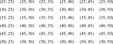
We want to assess the distribution of mean. The means of each of these samples are as below:

The histogram produced using MS Excel (Figure 5.9) exhibits the shape of the distribution for these sample means. The difference between the shape of the histogram between population and sample means (Figures 5.8 and 5.9) can be noticed easily and this leads to a very important result in inferential statistics. The distribution of sample means taken from the above population tends to be normal. An important question arises as to the shape of the distribution of sample means with differently shaped population distributions. The central limit theorem provides an answer to this question.

FIGURE 5.9 MS Excel produced histogram for sample means

5.10 Central Limit Theorem

According to the central limit theorem, if a population is normally distributed, the sample means for samples taken from that normal population are also normally distributed regardless of sample size. A population has a mean m and standard deviation s. If a sample of size n is drawn from the population, for sufficiently large sample size (n ≥ 30); the sample means are approximately normally distributed regardless of the shape of the population distribution.

Mathematically, it can be shown that the mean of the sample means is the population mean, that is, μ = and the standard deviation of the sample means is the standard deviation of the population, divided by the square root of the sample size, that is, . Central limit theorem is perhaps the most important theorem in statistical inference. The beauty of the central limit theorem lies in the fact that it allows a researcher to use the sample statistic to make an inference about the population parameter, even in cases where we have no idea about the shape of the distribution of the population. Central limit theorem provides a platform to apply normal distribution to many populations when the sample size is sufficiently large (n ≥ 30). In many situations, a researcher is not sure about the shape of the population distribution. Sometimes, a sample drawn from the population may not be distributed normally. In both the situations, if sample size is sufficiently large (n ≥ 30), the central limit theorem provides the opportunity of using the properties of normality.

Central limit theorem says that for sufficiently large sample size (n ≥ 30), the sample means are approximately normally distributed regardless of the shape of the population distribution. For a normally distributed population, sample means are normally distributed for any size of the sample. We have already discussed that the formula of determining z scores, for individual values from a normal distribution is

In case where sample means are normally distributed, z formula applied to sample mean will be

This formula is nothing but the general formula of obtaining z scores. In the formula, the mean of the statistic of interest is and the standard deviation of the statistic of interest is . This standard deviation is sometimes termed as the standard error of the mean. For computing , a researcher has to randomly draw all the possible samples of any given size, from the population; then, he has to compute sample mean from these samples. Practically this task is very difficult or some times even impossible within a specified period of time. Very fortunately, is equal to population mean which is relatively easy to compute. In a similar manner, for computing the value of , a researcher has to draw all the possible samples of any given size, from the population and has to compute the standard deviation accordingly. This task also faces the same degree of difficulty because for computing the standard deviation, a researcher has to calculate sample standard deviations from all the possible samples. Fortunately, is equal to the population standard deviation divided by the square root of the sample size. Substituting these two values in the above z formula, the revised version of the z formula can be presented as below:

As sample size increases, the standard deviation of the sample mean becomes smaller because the population standard deviation (s) is divided by the larger values of the square root of the sample size. Example 5.1 explains the application of the central limit theorem clearly.

Example 5.1

The distribution of the annual earnings of the employees of a cement factory is negatively skewed. This distribution has a mean of 25,000 and standard deviation of 3000. If a researcher draws a random sample of size 50, what is the probability that their average earnings will be more than 26,000?

Soultion

The z formula used for this problem is as below:

Here, Population mean (m) = 25,000

Population standard deviation (s ) = 3000

Sample size (n) = 50

Sample mean = 26,000

By substituting all these values in the z formula, we obtain the z score as below:

z = 2.35

This gives an area of 0.4906 between z = 0 to z = 2.35. This is an area between mean and 26,000. The required area lies between 26,000 and the area under the right-hand tail. So, the required area under normal curve is

(Area between 26,000 and the right hand tail) = (Area between the mean and right hand tail) – (Area between mean and 26,000)

Required area = 0.5000 – 0.4906 = 0.0094

Thus, the probability that the average earning of the sample group is more than 26,000 will be 0.94% (as shown in Figures 5.10 and 5.11).

Figure 5.10 Probability that the average earnings of employees is more than 26,000

Figure 5.11 Corresponding z scores for probability of average earnings more than 26,000

5.10.1 Case of Sampling from a Finite Population

Example 5.1 is based on the assumption that the population is extremely large or infinite. In case of a finite population, a statistical adjustment called finite correction factor can be incorporated into the z formula for sample mean. This correction factor is given by . It operates on standard deviation of the sample means, . After applying this finite correction factor, the z formula becomes

For example, a random sample of size 40 is taken from finite population of size 500. For this particular case, finite correction factor can be computed as

= = 0.96

In the above formula, standard deviation of the mean or standard error of the mean is adjusted downwards by using 0.96. As the size of the finite population becomes larger, as compared to the sample size, the finite correction approaches unity or 1. There exists a thumb rule for using the finite correction factor. If the sample size is less than 5% of the finite population size (symbolically ), the finite correction factor does not provide a significant modified solution.

Self-Practice Problems

5A1. A population has mean 100 and standard deviation 15. From this population, a random sample of size 25 is taken. Compute the following probabilities:

(a) Sample mean is greater than 90

(b) Sample mean is greater than 105

(c) Sample mean is less than 90

(d) Sample mean is less than 105

5A2. A researcher has taken a random sample of size 30 from a normally distributed population which has mean 150 and standard deviation 50. Compute the probability of obtaining sample mean more than 160. Also compute the probability of obtaining a sample mean less than or equal to 160.

5A3. In a big bazaar, the mean expenditure per customer is 1850 with a standard deviation of 750. If a random sample of 100 customers is selected, what is the probability that the, sample average expenditure per customer for this sample is more than 2000.

5.11 Sample distribution of sample proportion

When data items are measurable such as time, income, weight, height, etc. sample mean can be an appropriate statistic of choice. In cases where research produces countable items such as the number of people in a sample who own cars (and we want to estimate population proportion through sample proportion) the sample proportion can be an appropriate statistic. In many situations, the researcher uses sampling proportion to make the statistical inference about the population proportion p. The process of using sample proportion to make an inference about the population proportion p is exhibited in Figure 5.12.

Figure 5.12 Using sample proportion to make an inference about the population proportion p

The sampling distribution of is the probability distribution of all the possible values of the sample proportion . The sample proportion can be obtained by dividing the frequency with which a given characteristic occurs in a sample by the number of items in the sample. Symbolically,

Sample proportion

where x is the number of items in a sample possessing the given characteristics and n the number of items in the sample.

The mean of the sample proportion, for all the samples of size n drawn from a population is p (the population proportion) and the standard deviation of the sample proportion is After obtaining mean and standard deviation of the sample proportion, it is important to understand how a researcher can use the sample proportion in analysis. The concept of central limit theorem can also be applied to the sampling distribution of with certain conditions. For a large sample size, the sampling distribution of can be approximated by a normal probability distribution. Here, we need to understand which sample size can be considered large for applying the central limit theorem. Under two pre-specified circumstances np ≥ 5 and nq ≥ 5, the sample distribution of can be approximated by a normal distribution.

The z formula for sample proportion for np ≥ 5 and nq ≥ 5 is

where = 1 – p.

Example 5.2

In a population of razor blades, 15% are defective. What is the probability of randomly selecting 90 razor blades and finding 10 or less defective?

Soultion

Here, p = 0.15, = 90

By substituting all the values in the z formula

The z value obtained is –1.06 and the corresponding probability from the standard normal table is 0.3554, which is the area between sample proportion 0.11 and the population proportion 0.15 (as shown in Figure 5.13). So, the probability of randomly selecting 90 razor blades and finding 10 or less defective is

Figure 5.13 The probability of randomly selecting 90 razor blades and finding 10 or less defective

This result indicates that 10 or less razor blades will be defective in a random sample of 90 razor blades 14.46% of the time when the population proportion is 0.15.

Self-Practice Problems

5B1. The branded mattresses market has four product variants: rubberised coir, polyurethane, rubber foam, and spring mattresses. Rubberised coir mattresses occupy a market share of 63%.³ What is the probability of randomly selecting 150 customers and finding 90 of them or fewer using rubberised coir mattresses?

5B2. Hindustan Petroleum Company Ltd has an 18% market share in the lubricants market.³ What is the probability of randomly selecting 120 customers and finding 38 or more HPCL lubricant purchasers?

Example 5.3

In a grocery store, the mean expenditure per customer is 2000 with a standard deviation of 300. If a random sample of 50 customers is selected, what is the probability that the sample average expenditure per customer is more than 2080?

Soultion

As discussed in the chapter, the z formula is given as below:

Here, Population mean (m) = 2,000

Population standard deviation (s) = 300

Sample size (n) = 50

Sample mean = 2080

By substituting all these values in the z formula, we get the z score as below:

z = 1.88

So, the required area under normal curve is

 

(Area between z = 1.88 and the right-hand tail) = (Area between z = 0 and right-hand tail) – (Area between z = 0 and z = 1.88 )

Required area = 0.5000 – 0.4699 = 0.0301

Probability that sample average expenditure per customer is more than 2080 is 3.01% as shown in Figure 5.14.

Figure 5.14 Shaded area under the normal curve exhibiting the probability that sample average expenditure per customer is more than 2080

Example 5.4

For Example 5.3, determine the probability that the sample average expenditure per customer is between 2040 and 2080.

Soultion

In this problem, we have to determine . Sample mean is given as and .

For 2040,

For 2080, z = 1.88 (computed in Example 5.3)

From Figure 5.15 it is clear that we have to determine the area between z = 0.94 and z = 1.88

Figure 5.15 Shaded area under normal curve exhibiting the probability of sample average expenditure per customer between 2040 and 2080.

So, the required area under normal curve is

(Area between z = 0.94 and z = 1.88) = (Area between z = 0 and z = 1.88) – (Area between z = 0 and z = 0.94)

= 0.4699 – 0.3264 = 0.1435

The probability that the sample average expenditure is between 2040 and 2080 is 0.1435.

Example 5.5

The bottled water segment in India has witnessed rapid growth. Institutional users are responsible for 30% sales in the market.³ If 100 customers are randomly selected, what is the probability that 25 or more customers are institutional users?

Soultion

Here, p = 0.30, = 100

By substituting all the values in the z formula, we obtain

The z value obtained is –1.09 and the corresponding probability from the normal table is 0.3621, which is the area between sample proportion, 0.25 and the population proportion, 0.30. Figure 5.16 exhibits this area. So, when 100 customers are randomly selected, then the probability that 25 or more customers are institutional users is

Figure 5.16 Shaded area under the normal curve exhibiting the probability that 25 or more customers are institutional users.

This result indicates that 86.21% of the time a random sample of 100 customers will consist of 25 or more institutional users.

Example 5.6

By the year 2014–2015, the telephone instrument industry is estimated to grow by 106.20 million units as compared to 1993–1994 when the total market size was only 3 million units. Bharti Teletech, BPL Telecom, ITI (Indian Telephone Industries), Bharti Systel, Tata Telecom, and Gigrej Telecom are some of the major players in the market. Bharti Teletech has a market share of 24%.³ If 200 purchasers of telephone instruments are randomly selected, what is the probability that 55 or more are Bharti Teletech customers?

Soultion

In this example, p = 0.24, = 200

By substituting all the values in the z formula

The z value obtained is 1.16 and corresponding probability from the normal table is 0.3770. This is the area between z = 0 and z = 1.16. So, total area less than 1.16 is equal to 0.5000 = 0.8770. Hence, when 200 purchasers of telephone instruments are randomly selected, probability that 55 or more are Bharti Teletech customers is equal to 1 – 0.8770 = 0.1230 (Figure 5.17).

Figure 5.17 Shaded area under the normal curve exhibiting the probability that 55 or more are Bharti Teletech customers

SUMMARY

Due to various reasons, census or complete enumeration is not a feasible approach of obtaining information for conducting research or for any other purpose. Many researchers use a small portion of the population termed as a sample to make inferences about the population. The sampling process consists of five steps, namely determining target population; determining sampling frame; selecting appropriate sampling technique; determining sample size, and execution of the sampling process.

Sampling procedure can be broadly defined in two categories: random and non-random sampling. In random sampling, every unit of the population gets an equal probability of being selected in the sample. In non-random sampling, every unit of the population does not have the same chance of being selected in the sample. Simple random sampling, stratified random sampling, cluster sampling, and systematic sampling are some of the commonly used random sampling methods. Quota sampling, convenience sampling, judgement sampling, and snow ball sampling techniques are some of the commonly used non-random sampling techniques.

During any stage of research, the possibility of committing error cannot be eliminated. In statistics, these errors can be broadly classified under two categories: sampling errors and non-sampling errors. Sampling errors occur when the sample is not a true representative of the population. In complete enumeration, sampling errors are not present. Non-sampling errors are errors that arise not due to sampling but due to other factors in the process. Broadly, we can say that all errors other than sampling errors can be included in the category of non-sampling errors. Faulty designing and planning of the survey, response errors, non-response bias, errors in coverage, compiling, and publication errors are some of the common sources of non-sampling errors.

Sample mean is one of the most commonly used statistic in inferential process. This leads to a very important theorem of inferential statistics: the central limit theorem. Central limit theorem states that for a population with a mean m and standard deviation s, if a sample of size n is drawn from the population, for sufficiently large sample size (n ≥30), the sample means are approximately normally distributed regardless of the shape of the population distribution. If the population is normally distributed, the sample means are normally distributed for any size of the sample.

Key terms

Central limit theorem, 113

Cluster sampling, 106

Convenience sampling, 109

Judgement sampling, 109

Multi-stage sampling, 108

Non-random sampling, 100

Non-sampling errors, 99

Quota sampling, 109

Random sampling, 100

Sample, 98

Sampling, 98

Sampling error, 110

Sampling frame, 100

Simple random sampling, 101

Snowball sampling, 109

Stratified random sampling, 104

Systematic sampling, 107

Target population, 100

NOTES

1. Prowess (V. 3.1), Centre for Monitoring Indian Economy Ltd, Mumbai, accessed November 2008, reproduced with permission.
2. www.thehindu.com/2008/05/30/stories/200805 3056201700.htm, accessed November 2008.
3. www.indiastat.com, accessed November 2008, reproduced with permission.

Discussion questions

1. What is the difference between a sample and a census, and why is sampling so important for a researcher?
2. Explain the sampling design process.
3. What are sampling and non-sampling errors and how can a researcher control them?
4. Explain the types of probability or random sampling techniques.
5. Explain the types of non-probability or non-random sampling techniques.
6. How do probability sampling techniques or random sampling techniques differ from non-probability sampling techniques or non-random sampling techniques?
7. What is the concept of sampling distribution and also state its importance in inferential statistics?

Numerical problems

1. A population has mean 40 and standard deviation 10. A random sample of size 50 is taken from the population, what is the probability that the sample mean is each of the following:
   1. Greater than or equal to 42
   2. Less than 41
   3. Between 38 and 43
2. A housing board colony of Gwalior consists of 2000 houses. A researcher wants to know the average income of the households in this housing board colony. The mean income per household is 150,000 with standard deviation 15,000. A random sample of 200 households is selected by a researcher and analysed. What is the probability that the sample average is greater than 160,000?
3. A population proportion is 0.55. A random sample of size 500 is drawn from the population.
   1. What is the probability that sample proportion is greater than 0.58?
   2. What is the probability that sample proportion is ­between 0.5 and 0.6?
4. The government of a newly formed state in India is worried about the rising unemployment rates. It has promoted some finance companies to launch schemes to reduce the rate of unemployment by promoting entrepreneurial skills. A finance company introduced a scheme to finance young graduates to start their own business. Out of 200,000 young graduates, 130,000 accepted the policy and received loans. If a random sample of 20,000 is taken from the population, what is the probability that it exceeds 60% acceptance?
5. A market research firm has conducted a survey and found that 58% of the customers complete their important shopping on Sunday. Suppose 100 customers are randomly selected:
   1. What is the probability that 45 or more than 45 ­customers complete their important shopping on Sunday?
   2. What is the probability that 70 or more than 70 ­customers complete their important shopping on Sunday?

CASE STUDY

Case 5: Air Conditioner Industry in India: Systematic Replacement of the Unorganized Sector by the Organized Sector

Introduction

The Indian consumer durables industry is estimated to have a total market size of 250,000 million. The home appliances industry is estimated to have a size of 87,500 million. Refrigerators contribute to the largest share at around 38,000 million, followed by room air-conditioners at around 27,500 million, and washing machines at 14,000 million. The air-conditioner industry enjoys the highest growth in the appliances category and is expected to grow at over 20% in the years to come.¹ Due to the high prices in the organized sector, the unorganized sector was responsible for a lion’s share of the total sales until a few years ago. The reduction in excise duties and a decline in import duties have narrowed down the price gap in the unorganized and organized sectors

The share of the unorganized market, which was at 70% in the 1980s has dropped down and is now only 25%.² Increasing disposa-ble incomes and the change in lifestyles are some of the factors supporting the upward demand for air conditioners in the country. Table 5.01 exhibits the market share of air- conditioners in different categories and region-wise market share of air-conditioners. Table 5.02 shows the market share of air-conditioners in the organized and unorganized sectors for window and split air-conditioners. As is evident from Table 5.02, metro cities have 60% market share as compared to a group of non-metro cities that have a market share of 40%.

Major Players in the Market

An increased share in the market has allowed various major players to participate in the race for maximizing their own market share. Blue Star, LG, Voltas, Carrier, Amtrex Hitachi, Samsung, National, etc. are some of the major players in the market.

Blue Star, founded in 1949, is one of the major players in the market with an annual turnover of 22,700 million. Voltas was founded in 1951 as a collaboration between Tata Sons Ltd and a Swiss firm Volkart Brothers. Voltas’s domestic air-conditioning and refrigeration business witnessed a growth in revenue of 48% in 2006–2007 over the previous year. Carrier Aircon, an international major started operations in India in 1986, and established Carrier Refrigeration in 1992. Carrier has become an important player in the market in just a few years.

Table 5.01 Market share of air conditioners in different categories and region-wise market share of air conditioners

Hitachi Home & Life Solutions (India) Ltd, a subsidiary of Hitachi Home & Life Solutions Inc., Japan was established in 1984. On the basis of consumer research, the company launched an advanced “Logicool” range of ACs. LG Electronics, a major market shareholder has launched its new brand “LG Plasma” which filters out air in four stages. Market giants like National, Samsung, Videocon, and Whirlpool also have a sound footing in the market.

Table 5.02 Market share of air-conditioners in the organized and the informal sectors.

The Indian air-conditioner industry continues to register a growth of over 25%. There is a higher preference for split air-conditioners over window air-conditioners in the Indian market in line with the global trends. The household segment has shown a rapid increase and now accounts for 65% of the total market. The presence of more than 20 players in the market, including a few new entrants, both Indian and Chinese, has ensured that the selling price of air-conditioners has remained steady despite cost pressures.¹

Suppose you have been appointed as a business analyst by a leading multinational company preparing to enter the air-conditioners segment. You have been assigned the task of analysing the needs of customers with respect to product features:

1. What will be your sampling frame, appropriate sampling techniques, sample size, and sampling process?
2. Will you be using probability sampling technique or non-probability sampling technique and why?
3. What will be your plans to control sampling and non-sampling errors to obtain an accurate result?

NOTES

1. Prowess (V. 3.1), Centre for Monitoring Indian Economy Pvt. Ltd, Mumbai, accessed November 2008, reproduced with permission.
2. www.indiastat.com, accessed November 2008, reproduced with permission.