
Chapter 20
Sales Forecasting
Look to the future, because that is where you’ll spend the rest of your life.
– George Burns
Learning Objectives
Upon completion of this chapter, you will be able to:
- Understand the types of forecasting methods (qualitative and quantitative)
- Understand the concept, importance, and components of time series
- Understand the concept of measurement of errors in forecasting
- Understand how to use regression model for trend analysis
- Understand the concept of autocorrelation and autoregression and the use of autoregression in forecasting
- Understand the concept and importance of index numbers
STATISTICS IN ACTION: HINDUSTAN SANITARYWARE & INDUSTRIES LTD
The real estate sector in India has grown at an average rate of 30% over the last few years. The increase in disposable incomes, decline in interest rates, easy and flexible financing, superior real estate options, and relocation of foreign direct investment in construction and real estate are some of the factors responsible for the speedy growth. Apart from sustained economic growth, urbanization, high aspiration levels, and the increase in the number of nuclear families have also been responsible for the surge in housing demand. This trend is likely to sustain. The sanitaryware industry in India has witnessed accelerated growth rates as a result of the boom in the real estate sector.1
Hindustan Sanitaryware & Industries Ltd is the flagship company of the Somany group and was established in 1962 as a joint venture with Twyfords of the UK. In India, it soon pioneered vitreous china sanitaryware and gave the concept of sanitaryware a new meaning. The company’s brand, “Hindware” commands more than one-third share of the Indian sanitaryware market and is a leader in several categories. It is recognized among the top 300 companies in the country and is also rated among the 100 best small- and medium-sized companies in the world by Forbes Magazine.2 Table 20.1 provides the net income of the company from 1995–2007.
TABLE 20.1 Net income of Hindustan Sanitaryware & Industries Ltd from 1995–2007

Source: Prowess (V. 3.1), Centre for Monitoring Indian Economy Pvt. Ltd, Mumbai, accessed September 2008, reproduced with permission.
It is possible to forecast the sales of the company in the forthcoming years using statistical forecasting techniques. This chapter mainly focuses on the different types of forecasting methods; concept of time series and measurement of error in forecasting; use of regression models for trend analysis; concept of autocorrelation and autoregression, and the use of autoregression in forecasting. The concept and importance of index numbers is also discussed in detail.
20.1 INTRODUCTION
In today’s highly dynamic business environment, managers have to forecast the future and design strategies accordingly. Managers use forecasting (the art or science of predicting the future) techniques to make strategic decisions about selling, buying, hiring, etc every day. The past data are used by managers to make predictions about the future. For example, let us assume that a company wants to order raw material in advance for its production processes in the current year. The demand for the finished product is uncertain in the current year. In this situation, the company can take the help of forecasting techniques (with the help of past data) to order inventory for the current year. These techniques are discussed in detail in this chapter.
In modern organizations, managers believe in being proactive. This proactive approach is based on future planning. Forecasting is a technique which can aid in future planning. Time series is an important tool that can be used to predict the future. The future is always uncertain, but with the help of past data, an assessment of the future can be made. That is precisely why time series analysis is very important in the fields of economics, sales, and production. Time series analysis is also helpful in making predictions about population, national income, capital formation, etc. The main objective in analysing time series is to understand, interpret, and evaluate changes in economic phenomena in the hope of anticipating the course of future events correctly.
20.2 TYPES OF FORECASTING METHODS
In general, there are two common ways of forecasting. These are—qualitative forecasting and quantitative forecasting methods. Figure 20.1 exhibits these methods of forecasting.

FIGURE 20.1 Methods of forecasting
20.3 QUALITATIVE METHODS OF FORECASTING
Companies have to rely on qualitative methods of forecasting when historical data are not available. These methods are subjective and judgemental in nature. As described in Figure 20.1, executive opinion, panel judgement, delphi method, marketing research, and past analogy methods can be included in this category.
In the executive opinion method, the experience of executives is used to predict the future. For example, if past data are unavailable, the experience of sales executives in the market can be used to forecast sales in the future. Executive opinion method may suffer from errors due to individual bias. The panel judgement method is used to tackle problems that result on account of individual bias. In the panel judgement method, a panel of individuals who are knowledgeable about the subject is constituted. This panel of individuals share information and opinions about the matter under study and arrive at a conclusion. In the Delphi method, a group of experts who may be stationed at different locations and who do not interact with each other is constituted. After this, a questionnaire is sent to each expert to seek his opinion about the matter under investigation. A summary is prepared on the basis of the returned questionnaire. On the basis of this summary, a few more questions are included in the questionnaire and this modified questionnaire is again sent back to each expert. This process is repeated until a desired consensus is arrived. In the marketing research method, a well-designed questionnaire is prepared and distributed among respondents. On the basis of response obtained, a summary is prepared and the survey result is developed. In the past analogy method, the past sales trends of other products are used to forecast sales. These other products may be substitute products, complementary products, or products belonging to consumers in the same income group.
Quantitative methods of forecasting can be broadly divided into two categories: Time series analysis and Causal analysis. Time series analysis involves the projection of the future on the basis of the information available currently. Causal analysis is based on the cause and effect relationship between the two or more variables under study.
Quantitative methods of forecasting can be broadly divided into two categories: Time series analysis and Causal analysis. Time series analysis involves the projection of the future on the basis of the information available currently. Causal analysis is based on the cause and effect relationship between two or more variables under study.
20.4 TIME SERIES ANALYSIS
There are various methods of arranging statistical data. Data can be arranged according to size, geographic area, time of occurrence, etc. The arrangement of statistical data in accordance with the time of occurrence or the arrangement of data in chronological order is known as a time series. This time span may be an hour, a week, a month, a year or several years, depending upon the type of event to which the data refers. In other words, a time series may be defined as a collection of numerical values of variables obtained over regular periods of time.
Mathematically, a time series can be defined by the functional relationship
yt = f (t)
where yt is the value of a variable (or phenomenon) over time period t. For example, (i) sales (yt) of a consumer durables company in different months (t) of the year (ii) the temperature of a place (yt) on different days (t) of the week. Thus, if the values of a variable at time period t1, t2, t3, …, tn are y1, y2, y3, …, yn, then the series
t = t1, t2, t3, …, tn
yt = y1, y2, y3, …, yn
constitute a time series. For example, sales (yt) of a consumer durables company in different years (t) constitute a time series. Table 20.2 gives the sales of a consumer durable company from 1995–2004.
TABLE 20.2 Sales (yt) of a consumer durables company in different years (t)
Thus, a time series is a bivariate distribution, in which one variable is time and the other variable is the value of a variable (or phenomenon) for different time periods. Figure 20.2 exhibits the time series plot of sales for a consumer durables company produced using Minitab.
FIGURE 20.2 Time series plot of sales for a consumer durables company produced using Minitab
A time series may be defined as a collection of numerical values of some variable obtained over regular periods of time.
20.5 Components of Time Series
In a time series, data are based on time. Therefore, it is natural that the variable under consideration will change from time to time. A single force cannot be held responsible for fluctuations in data. On the other hand, the net effect of multiplicity of forces seem to be responsible for fluctuations in data. If these forces remain in equilibrium, the resulting time series will remain constant. For example, the sales of a consumer electronics company is influenced by a number of forces rather than a single force. These forces may be a change in the purchasing power of an individual, supply of the finished product by the company, advertising campaigns at a particular time, effort of the sales force, price and quantity discounts offered by the company, etc. The factors that cause fluctuations may be classified into four different categories called the components of time series. Generally in a long time series, the following four components are found to be present.
1. Secular trend or long term movements
2. Seasonal variations
3. Cyclic variations
4. Random or irregular movements
20.5.1 Secular Trend
Secular trend or simple trend indicates the general tendency of the data to increase or decrease over a long period of time. For example, an upward tendency is usually observed in the data pertaining to population, production, sales, price or income. On the other hand, a downward tendency can be observed in the data pertaining to the rate of infant mortality, the decrease in deaths due to epidemics owing to advancements in medical facilities, etc.
It is not necessary that the increase or decrease be in the same direction throughout the given time period. Different tendencies of increase or decrease or stability can be observed over different periods of time; however, the overall tendency may be upward downward or stable. This does not mean that all the series must show upward or downward trend. In some cases, values may fluctuate around a constant reading, which does not change with time. For example, the temperature of a particular place does not vary too much with time, instead it remains constant (fluctuates mildly) with time (when the temperature for the different days of a week are considered).
The term “long period of time” is a relative term and cannot be defined exactly. In some cases, 2 weeks may be a long period of time. On the other hand, in some case 2 weeks may not be considered a long period. For example, in order to control an epidemic, 1 week is considered a fairly “long period of time,” however, for a census, 1 week cannot be considered a “long period of time.”
If the values of a time series are plotted on a graph and these values cluster more or less around a straight line, then the trend shown by the straight line is termed as linear, otherwise the trend is termed as a non-linear trend.
Secular trend or simply trend indicates the general tendency of the data to increase or decrease over a long period of time.
20.5.2 Seasonal Variations
There are variations in a time series due to rhythmic forces which operate in a repetitive, predictable, and periodic manner in a time span of one year or less. Thus, seasonal fluctuations can be measured only if the data are recorded hourly, daily, weekly, monthly, quarterly (every three months). In seasonal variations, the time period should not exceed one year. Most economic series are influenced by seasonal variations. For example, sales of umbrellas and rain coats pick up in the rainy season, sales of ice-cream pick up in the summer, the sales of gold ornaments zoom up during the wedding season, etc.
The study of seasonal variations are important for three reasons. First, we can establish the pattern of past changes. Second, the projection of past patterns into the future is a useful technique of prediction. Third, the effects of seasonal variations can be eliminated from the time series after their presence is established.
Seasonal variations can be of two types:
(i) Seasonal variations due to natural forces: There are seasonal variations in the time series due to weather conditions and climatic changes. For example, sales of umbrellas and rain coats zoom up during the rainy reason, sale of ice-creams zoom up in summer, sales of woollen clothes pick up during the winter, the demand for electric fans and air-conditioners goes up during summer, etc. All these variations are due to seasons and can be predicted up to an extent.
Seasonal variations are the variations in time series due to rhythmic forces which operate in a repetitive, predictable, and periodic manner in a time span of one year or less.
(ii) Seasonal variations due to customs: There are seasonal variations due to customs, habits, lifestyle, and conventions of the people in a society. For example, sales of paints and distempers pick up just before Diwali, sales of jewellery and ornaments go up around the marriage season, sales of sweets go up during festivals such as Diwali, Dushera, Holi, Rakshabandhan, etc.
The study of seasonal variations is of paramount importance for businessmen and sales managers. For example, the sales manager of a fast moving consumer goods company has to make policies for purchase, production, inventory control, personnel requirement, advertising, and sales promotion techniques. In order to formulate policies, the knowledge of seasonal variations is very important. Without the knowledge of these seasonal fluctuations, the sales manager may commit mistakes in judging seasonal upswings and seasonal slumps that may affect demand. Therefore, for understanding the behaviour of the phenomenon in a time series, the data must be adjusted for seasonal variations. This technique is called de-personalization and will be discussed later in this chapter.
20.5.3 Cyclical Variations
Cyclical variations refer to oscillatory movements in a time series with a period of oscillation of more than a year. Cyclical variations are the components of a time series that tend to oscillate above and below the secular trend line for periods longer than 1 year or 12 months. Cyclical variations are not as regular as seasonal variations. Instead they exhibit semi-regular periodicity. Most business and economic series represent intervals of prosperity, recession, depression, and recovery, which may also be referred as the “four phase cycle.” Each phase changes gradually into the phase that follows it in the given order. In a business activity, these phases follow one another with steady regularity. The period from the peak of one boom to the peak of the next boom is called a complete cycle. Most economic and commercial series relating to prices, production, income, etc. show this tendency. Cyclical variations are not periodic but more or less regular in nature.
Cyclical variations refer to oscillatory movements of time series with a period of oscillation of more than a year.
20.5.4 Random or Erratic or Irregular Variations
Apart from the three types of variations discussed above, a time series contains another factor which does not repeat in a definite pattern. These are called random or erratic or irregular variations. These variations are purely random, unforeseen, unstoppable, and unpredictable. Variations on account of calamities such as earthquakes, floods, famines, epidemics, etc. are beyond human control. Variations that arise in a time series due to specific events or episodes are called episodic variations. For example, natural calamities, fire, flood, etc. can be placed in the category of episodic variations. Figure 20.3 exhibits all the four components of a time series.

FIGURE 20.3 Components of a time series
Random or irregular variations are factors in a time series that do not repeat in a definite pattern and are random, unforeseen, unstoppable, and unpredictable.
20.6 TIME SERIES DECOMPOSITION MODELS
The analysis of time series includes the decomposition of the time series into trend (T ), seasonal variations (S ), cyclical variations (C ), and irregular or random variation (R). The main objective of time series decomposition is to isolate, study, analyse, and measure the components of time series independently and to determine the relative impact of each on the overall behaviour of the time series. Many models are available by which a time series can be analysed. Two models, commonly used for decomposing the time series into its components are the additive model and the multiplicative model.
The analysis of time series includes the decomposition of the time series into trend (T), seasonal variations (S), cyclical variations, (C) and irregular or random variation (R). The main objective of time series decomposition is to isolate, study, analyse, and measure the components of time series independently and to determine the relative impact of each on the overall behaviour of the time series.
20.6.1 The Additive Model
The additive model is used when it is assumed that the four components of a time series are independent of one another. This assumption may not hold true in a real-life time series. These components are considered independent of one another when the occurrence and the magnitude of movements in a particular component do not affect the other components. According to the additive model, a time series can be expressed as
Yi = Ti + Si + Ci + Ri
where Yi is the time series value at time i and Ti, Si, Ci, and Ri represent the values of trend, seasonal, cyclic, and random components of the time series at time i. This model also assumes that the different components are absolute quantities expressed in original units and can take positive and negative values. The cyclical variations will take positive or negative signs subject to their positions in terms of above or below the corresponding trend values. Positive values of cyclical variations during the upswing will wipe out the negative values, so that the net result over a period of the cycle is zero. Likewise, the net result of a seasonal variation in a year would also be zero.
The additive model is used when it is assumed that the four components of a time series are independent of one another. These components are termed independent of one another when the occurrence and the magnitude of movements in any particular component do not affect the other components.
20.6.2 The Multiplicative Model
In a multiplicative model, it is assumed that all the four components of time series are not independent and the overall variation in the time series is the combined result of the interaction of all the forces operating on the time series. According to the multiplicative model:
Yi = Ti × Si × Ci × Ri
where Yi is the time series value at time i and Ti, Si, Ci, and Ri represent the values of trend, seasonal, cyclic, and random components at time i.
In a multiplicative model, it is assumed that all the four components of a time series are not independent and the overall variation in the time series is the combined result of the interaction of all the forces operating on the time series.
By taking logarithms on both the sides of the above equation, we get
Log Yi = Log Ti + Log Si + Log Ci + Log Ri
Therefore, it is very clear that the multiplicative decomposition of time series is the same as the additive decomposition of time series with logarithmic values. In the multiplicative model, the geometric means of Si in a year, Ci in a cycle, and Ri in a long period of time are unity. Si, Ci, and Ri are index values fluctuating above or below unity. It is not necessary that all the four components be present in a time series. For example, in case of annual data, seasonal component is not present; likewise cyclical component is not present for relatively short period data. In the first case, the multiplicative model is Yi = Ti × Ci × Ri and in the second case, the multiplicative model is Yi = Ti × Si × Ri.
20.7 THE MEASUREMENT OF ERRORS IN FORECASTING
This chapter focuses on several forecasting techniques. In real life, a decision maker encounters the problem of selecting the best technique out of several available techniques. A decision maker has to select a technique that predicts the future well. One method of selecting a best technique is to compare the actual values with the forecasted values and compute the error in estimation. The techniques used to measure errors in forecasting are: mean absolute deviation (MAD), mean absolute percentage error (MAPE), and mean squared deviation (MSD).
In real life, a decision maker encounters the problem of selecting the best technique out of several available techniques. A decision maker has to select a technique that predicts the future well. One method of selecting a best technique is to compare the actual values with the forecasted values and compute the error in estimation. The techniques used to measure errors in forecasting are: mean absolute deviation (MAD), mean absolute percentage error (MAPE), and mean squared deviation (MSD).
The error of a forecast is the difference between the actual value and the forecasted value. Mathematically, an error in forecasting can be explained by
![]()
where ei is the error of the forecast, yi the actual value, and ![]() the forecasted value.
the forecasted value.
The three measures of accuracy—mean absolute deviation (MAD), mean absolute percentage error (MAPE), and mean squared deviation (MSD) can be computed as below:
Mean absolute deviation (MAD) =
Mean absolute percentage error (MAPE) =  × 100
× 100
Mean squared deviation (MSD) = 
Let us take the example of the consumer durables company again for understanding the concept of errors in forecasting. Table 20.3 exhibits the computation of the mean absolute deviation (MAD), the mean absolute percentage error (MAPE), and the mean squared deviation (MSD) for the consumer durables company.
TABLE 20.3 Computation of the mean absolute deviation (MAD), the mean absolute percentage error (MAPE), and the mean squared deviation (MSD) for the example relating to the consumer durables company
![]()
![]()
![]()
Mean absolute deviation (MAD) = ![]()
Mean absolute percentage error (MAPE) = ![]()
Mean squared deviation (MSD) = ![]()
Note: In Table 20.3, the third column indicates the forecasted value ![]() . The procedure of computing forecasted value
. The procedure of computing forecasted value ![]() is discussed later in this chapter. Mean absolute percentage error measures accuracy in terms of percentage values.
is discussed later in this chapter. Mean absolute percentage error measures accuracy in terms of percentage values.
20.8 QUANTITATIVE METHODS OF FORECASTING
Quantitative methods of forecasting are based on projecting past patterns of data to obtain a future forecast using some mathematical formulae. This method fails to describe the cause– effect relationship between variables. This drawback can be overcome by using causal analysis, which is based on the cause and effect relationship between two or more variables under study. Quantitative methods of time series forecasting can be broadly classified into three categories: free hand methods, smoothing methods, and exponential smoothing methods.
Quantitative methods of time series forecasting can be broadly classified into three categories: free hand methods, smoothing methods, and exponential smoothing methods.
20.9 Freehand method
The freehand method is the simplest method of determining trend. A freehand smooth curve is obtained by plotting the values yi against time i as shown in Figure 20.4. Smoothing of the time series with the freehand curve eliminates the seasonal and irregular components. This method is free from mathematical complexities and saves time. Therefore, results can be obtained very quickly. Though this method is very simple, it is not free from demerits. This method is too subjective. If same data is provided to two different persons, two different trend lines may be obtained. For drawing a best-fit trend line, experienced and skilled people are required. Since the trend line depends on human hands, human bias in drawing a trend line cannot be eliminated. In addition, this method does not measure trend mathematically.
The freehand method is the simplest method of determining trend. A freehand smooth curve is obtained by plotting the values yi against time i.

FIGURE 20.4 Freehand graph of sales with trend line for the example on the consumer durables company
While drawing a trend line by the freehand method, one should keep the following points in mind. First, the sum of vertical deviation of the observations above the trend line should be equal to the sum of the vertical deviation of the observations below the trend line. Second, the sum of squares of the vertical deviations of the observations from the trend line should be as less as possible. Third, the trend line should be drawn in such a way so that the trend line bisects the same area above and below a cycle.
20.10 SMOOTHING TECHNIQUES
The main objective of the smoothing technique is to “smooth out” the random variations due to the irregular fluctuation in the time-series data. Various methods are available to smooth out the random variations due to irregular fluctuations, so that the resulting series may have a better overall impression of the pattern of movement in the data over a specified period. In this section, we will focus on three methods of smoothing: moving averages method, weighted moving averages method, and semi- averages method.
The main objective of the smoothing technique is to smooth out the random variations due to the irregular fluctuations in the time-series data.
20.10.1 Moving Averages Method
The method of averages is used in the moving average technique to smooth out the irregularities in a time-series data. This method is highly subjective and depends upon the length of the period (L) selected for constructing the averages. For example, if we want to compute a 3-year moving average from a time series which contains 9 years, that is, n = 9, we have to add the first three values pertaining to the first three years as shown below:
![]()
Similarly, the second-moving average can be computed by taking the average pertaining to the next three values leaving the first one, that is,
![]()
This process continues until the computation of the last moving average as
![]()
Example 20.1 explains this process clearly.
Example 20.1
Table 20.4provides the sales of a manufacturing company in all the 12 months of 2006. Compute a three-month moving average for this time series.
TABLE 20.4 Sales turnover of a manufacturing company for 12 months in 2006
Solution The first 3-month moving average can be computed as
3-month moving average = ![]()
The other moving averages can be computed in a similar manner.
The actual sales for the month of April is ![]() 24 million and the forecasted sales is
24 million and the forecasted sales is ![]() 19.6667 million. Hence, the error of the forecast is computed as
19.6667 million. Hence, the error of the forecast is computed as
Error (for the month April) = 24 – 19.6667 = 4.3333
From Table 20.5 we can see that the first moving average value 19.6667 is displayed against April because this is the moving average value of the first three months: January, February, and March. Similarly, the second moving average value is the average sales in the months of February, March, and April. This value is placed against the month of May. The error is the difference between the actual sales and the forecasted sales. The errors are also indicated in Table 20.5. The 3-month moving average plot for Example 20.1 produced using Minitab is depicted in Figure 20.5.

FIGURE 20.5 3-month moving average plot for Example 20.1 produced using Minitab
TABLE 20.5 Computation of three-month moving average for Example 20.1
20.10.2 Weighted Moving Averages Method
We have already noticed that in the moving averages method, equal weights are assigned to all the time periods. There may be cases when a forecaster may want to attach different weights to different time periods according to their importance. Weighted moving averages method provides a forecaster the opportunity to weigh time periods based on their importance. So, in weighted moving averages method, the weight assignments to different time periods are somewhat arbitrary. In the absence of any specific formula for determining the weights, a general rule is used. As per this rule, the most recent observation of a time series receives more weight and the weights decrease for older values of the data.
For example, for computing the 3-month weighted moving average (the value which is placed against April) in Example 20.1, the value corresponding to March is multiplied by 3, the value corresponding to February is multiplied by 2, and the value corresponding to January is multiplied by 1. This weighted moving averages is computed as
![]()
where Mt – 1 is most recent month’s value, Mt – 2 the value for the previous month, Mt – 3 the value for the month before the previous month.
In the above formula, the denominator 6 is the sum of three weights, that is, the denominator is (3 + 2 + 1 = 6).
Example 20.2
Compute the 3-month weighted moving average value for the data given in Example 20.1. Weight the most recent month by 3, the previous month by 2, and the month before the previous month by 1.
Solution The weighted moving average can be computed by using the formula
![]()
For April, the weighted moving average can be computed as
![]() = 19.6667
= 19.6667
Similarly, for May, the weighted moving average can be computed as
![]()
In a similar manner, the weighted moving average for other months can be computed. These weighted moving averages are shown in Table 20.6.
TABLE 20.6 Computation of 3-month weighted moving average for Example 20.2
The general computational tools available with MS Excel, Minitab, and SPSS can be used for calculating weighted moving average.
20.10.2 Semi-Averages Method
In the semi-averages method, data are divided into two equal parts with respect to time. For example, consider a time series i, given from 1991–2000, that is, time is given over a period of 10 years. Then, the two equal parts of the data will be the time period from 1991–1995 and the time period from 1996–2000. If the time units in a time series are odd, then two equal parts would be obtained by dropping the value corresponding to the middle year and then dividing the remaining data into two equal parts. For example, for any time series i, given from 1991–1999, that is, time is given for a period of 9 years. The two equal parts would be the time period from 1991–1994 and time period from 1996–1999. The value corresponding to the middle year 1995 is dropped. The next step is to calculate the arithmetic mean for each part. Then this mean is plotted against the mid values of the respective time periods for each part. The line which is obtained by joining these two points is known as the trend line and can be extended to estimate future value. For even number of years, that is, for n = 12, (say time period from 1991–2002), data can be divided into two equal parts, that is, time slot from 1991–1996 and time slot from 1997–2002. The mean values for 1991–1996 and 1997–2002 are obtained and the first mean value is plotted against middle point of 1991–1996. This middle point will be the middle point of 1993 and 1994, that is, this middle point would be 1st July 1993. The same process should be followed for the second part of the data, that is, for the time span 1997–2002.
The intercept and slope of the trend line can also be obtained using this method. The arithmetic mean of the first part is the intercept value of the trend line. The slope of the trend line can be obtained by taking the ratio of the difference between two arithmetic means computed for two parts and the difference between years (against which arithmetic means are plotted).
In the semi-averages method, data is divided into two equal parts with respect to time.
Example 20.3
Determine straight line trend by semi-averages method for the time-series data related to production of a toy manufacturing company provided in Table 20.7. Also determine the projected production for 2005.
TABLE 20.7 Time-series data related to production of a toy manufacturing company
Solution According to the semi-averages method, the times series is divided into two equal parts. Here, the number of years are 10; hence, the first part would be the time slot from 1991–1995 and second part would be the time slot from 1996–2000.
The average of the first five years (from 1991–1995)
= ![]() (109 + 119 + 129 + 140 +153)
(109 + 119 + 129 + 140 +153)
= 130
The average of the second five years (from 1996–2000)
= ![]() (152 + 151 + 163 + 175 + 184)
(152 + 151 + 163 + 175 + 184)
= 165
The first average value is plotted against the middle year between 1991 and 1995, that is, against 1993 and the second average value is plotted against middle year between 1996–2000, that is, against 1998. For computing the time series y = a + bx, we need to compute the values of intercept a and slope b as under:
Slope of the trend line (b) = ![]()
As discussed earlier intercept (a) = 130 units (arithmetic mean of the first part)
The resultant trend line can be obtained by substituting the values of a and b in the equation y = a + bx. Thus, the required trend line is
y = 130 + 7 × (x)
For the year 2005 (which is 12 years away from the origin year 1993) the projected production can be computed as:
y = 130 + 7 × (12) = 214
Figure 20.6 exhibits the time series plot of production (trend line obtained by the method of semi-averages).
FIGURE 20.6 Time series plot of production (trend line obtained by the method of semi-averages) for Example 20.3

20.11 EXPONENTIAL SMOOTHING METHOD
Exponential smoothing is another technique used to “smooth” a time series. Exponential smoothing is a type of moving average technique which consists of a series of exponentially weighted moving averages. The exponential smoothing method weigh data from the previous time period with exponentially decreasing importance in the forecast. This method has a relative advantage over the methods of moving averages discussed previously. First, this method focuses upon the most recent data (data from the previous time period with exponentially decreasing importance in the forecast). Second, during forecasting, this method takes into account all the observed values because each smoothing value is based upon the values observed previously. In this manner, the values observed most recently receive the highest weight; the previously observed value receives the second highest weight and so on.
Exponential smoothing methods weigh data from the previous time period with expo nentially decreasing importance in the forecast.
In exponential smoothing method, forecasting is carried out by multiplying the actual value for the present time period, Xt, by a value between 0 and 1 (the exponential smoothing constant). This exponential constant is referred to as α (not the same α used in Type I error). So, the resultant value is α . Xt. This value α . Xt is added to the product of the present time period forecast Ft and (1 – α). Algebraically, this formula can be stated as below:
Ft + 1 = α . Xt + (1 – α) . Ft
where Ft + 1 is the forecast for the next time period (t + 1), Ft the forecast for the present time period (t), α the exponential smoothing constant (0≤ α ≤1), and Xt the actual value for the present time period (t).
The choice of exponential smoothing constant is a very critical step because it directly affects the result. The selection of the exponential smoothing constant is subjective. From the formula given above, we see that the forecast for the next time period is a combination of the actual value for the present time period and the forecast for the present time period. If a forecaster selects α less than 0.5, less weight is placed on the actual value for the present time period and greater weight is placed on the forecast for the present time period. If a forecaster wants to eliminate unwanted cyclical and irregular fluctuations, he or she should select a small value of α (closer to 0). In this case, the overall long term tendencies of the series will be more apparent. If the objective is only forecasting, large value of α (close to 1) should be selected. In this manner, future short-term directions may be more accurately predicted.
In order to understand why this procedure is called exponential smoothing, the formula for forecasting the value of the next time period (t + 1) is taken once more as
Ft + 1 = α . Xt + (1 – α) . Ft
If we want to forecast the value of the present time period (t), the forecast Ft is obtained by
Ft = α . Xt – 1 + (1 – α) . Ft – 1
By substituting the value of Ft in the above equation of forecasting Ft + 1, we get
Ft + 1 = α . Xt + (1 – α) . [α . Xt – 1 + (1 – α) . Ft – 1]
We know that Ft – 1 = α . Xt – 2 + (1 – α) . Ft – 2
Substituting this value of Ft – 1 in the preceding equation for Ft + 1, we get
![]()
![]()
We have discussed that exponential smoothing method weigh data from the previous time period with exponentially decreasing importance in the forecast. This concept is explained by Table 20.8 which contains different values of α and related changes in the values of ![]() and
and ![]() .
.
TABLE 20.8 Different values of α and related changes in the values of α . (1 – α) ; α . (1 – α)2; α . (1 – α)3 , and α . (1 – α)4
The exponential formula Ft + 1 = α . X t + (1 – α). Ft can be rearranged as Ft + 1 ![]() . In this type of arrangement (Xt – Ft), that is, the difference between actual values and forecasted values is referred to as the forecast error. The formula given above clearly shows that the new forecast is equal to the old forecast Ft, plus an adjustment based on α times forecasted error.
. In this type of arrangement (Xt – Ft), that is, the difference between actual values and forecasted values is referred to as the forecast error. The formula given above clearly shows that the new forecast is equal to the old forecast Ft, plus an adjustment based on α times forecasted error.
Example 20.4
Table 20.9 gives the number of units produced by a watch manufacturing company in different years.
TABLE 20.9 Units produced by a watch manufacturing company in different years
Use exponential smoothing method with α = 0.3, α = 0.5, and α = 0.7 to forecast the production of watches.
Solution Table 20.10 provides the production forecast for three different values of α. It can be seen from the table that since no forecast is given for the first time period, the forecast based on exponential smoothing method for the second time period cannot be computed. The actual value of the first time period is used to forecast the value of second time period to initiate the procedure. Figure 20.7 shows the Minitab time series plot of production for Example 20.4.

FIGURE 20.7 Time series plot of production (actual values) for Example 20.4 produced using Minitab
TABLE 20.10 Production forecasts for three different values of α
Figure 20.8, 20.9 and 20.10 exhibit the Minitab produced exponential smoothing plots for different values of α (α = 0.3, α = 0.5, and α = 0.7). If we compare the three accuracy measures given with the three plots, we find that all the three measures are less for the highest value of α, that is, for 0.7. Figure 20.10 clearly exhibits that the actual values vary considerably with the largest value of α seeming to forecast the best.

FIGURE 20.8 Exponential smoothing plot for Example 20.4 when α = 0.3, produced using Minitab

FIGURE 20.9 Exponential smoothing plot for Example 20.4 when α = 0.5, produced using Minitab

FIGURE 20.10 Exponential smoothing plot for Example 20.4 when α = 0.7, produced using Minitab
20.12 Double Exponential Smoothing
Single exponential smoothing does not incorporate trend and seasonal components of time series data. There are techniques by which trend and seasonal components can be incorporated in a time series, subject to their existence. In this section, we will focus upon the exponential smoothing method which considers trend effects in forecasting. Holt’s two parameter technique is a technique which includes trend effects in forecasting. Holt’s double exponential smoothing method for a period t is given by
Forecast for the next period (Ft+1) = Et + Tt
where, Et = α. Xt + (1 – α) (Et–1 + Tt–1)
and Tt = β (Et – Et–1) + (1 – β) Tt–1
Forecast for k periods in future = Et + kTt
Since the trend component is also included in the process, one more smoothing constant β is included in the process. Therefore, Holt’s method uses two smoothing constants α and β. These two weights can be the same or different. As discussed earlier, higher values of α and β will give more emphasis on recent values. To forecast the next period (Ft+1) = Et + Tt is used. In order to forecast more than one period in the future, use Et + kTt, where k is the number of periods in future to be forecasted. For example, the forecast for the next four periods is given by
Ft+1 = Et + 4Tt
Single exponential smoothing does not incorporate trend and seasonal components of time series data. Holt’s two parameter technique is a technique which includes trend effects in forecasting.
While calculating the new smoothed value using Et = α Xt + (1 – α) (Et–1 + Tt–1), the last term is simply a forecast for this period. When we substitute Ft = Et–1 + Tt–1 in the above formula, we get Et = α Xt + (1 – α) Ft.
Let us solve Example 20.4 again by using Holt’s two parameter technique. Holt’s method uses two smoothing constants α and β, α is taken as 0.8 and β is taken as 0.4. The initial values are taken as E1996 = 120 and T1996 = 0. The forecast for the year 1997 can be obtained as
F1997 = E1996 + T1996 = 120 + 0 = 120
The forecast for 1998 can be obtained as
F1998 = E1997 + T1997
where E1997 can be computed as
E1997 = (0.8) × X1997 + (1 – 0.8) × F1997 = (0.8) × (112) + (0.2) × 120 = 89.6 + 24 = 113.6
T1997 can be computed as
T1997 = (0.4) × (E1997 – E1996) + (1 – 0.4) T1996 = (0.4) × (113.6 – 120) + (0.6) × 0 = –2.56
Hence, F1998 = E1997 + T1997 = 113.6 – 2.56 = 111.04
The forecast for 1999 can be obtained as
F1999 = E1998 + T1998
E1998 can be computed as
E1998 = (0.8) × X1998 + (1 – 0.8) × F1998 = (0.8) × (136) + (0.2) × (111.04)
= 108.8 + 22.208 = 131.008
T1998 can be computed as
T1998 = (0.4) × (E1998 – E1997) + (1 – 0.4) T1997 = (0.4) × (131.008 – 113.6) + (0.6) × (–2.56) = 5.42
Hence, F1999 = E1998 + T1998 = 131.008 + 5.42
= 136.428
Other forecasted values can be calculated similarly.
20.11.1 Using SPSS for Holt’s Method
Click Analyze/Time Series/Exponential Smoothing. The Exponential Smoothing dialog box will appear on the screen (Figure 20.13). Place Production in the Variables box. From Model, select Holt and click Parameters. The Exponential Smoothing: Parameters dialog box will appear on the screen (Figure 20.14). From General (Alpha) box, select Value and place the value of α = 0.8 in the box. From Trend (Gamma) box, select Value and place the value of β = 0.4 in the box. From the “Initial Values” box, click Custom and place 120 in the Starting box and 0 in the Trend box. Click Continue, the Exponential Smoothing dialog box will reappear on the screen. Click OK, SPSS output as shown in Figures 20.11 and 20.12 will appear on the screen. Fits and errors will be attached with the data sheet as shown in Figure 20.11.

FIGURE 20.11 SPSS output with data sheet for Example 20.4 (using Holt’s method)

FIGURE 20.12 SPSS output for Example 20.4 (using Holt’s method)

FIGURE 20.13 SPSS Exponential Smoothing dialog box
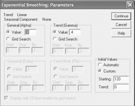
FIGURE 20.14 SPSS Exponential Smoothing: Parameters dialog box
Self-Practice Problems
20A1. The following data provides the sales of a consumer durable company from 1992–2003. Compute a 3-year moving average for this time series.
20A2. Compute 3-year weighted moving average values for Example 20A1. Use weight 3 for last year’s value, weight 2 for the previous year’s value, and weight 1 for the year before the previous year’s value.
20A3. Pfizer Ltd, a US-based company, commenced operations in India in 1950 as private ltd company under the name Dumex Ltd in Mumbai. Pfizer India’s business is segregated into three different groups. Pharmaceuticals accounted for the bulk (87%) of the company’s revenues in 2007 while its animal health business chipped in 10%. Its service business contributed the remaining 3%.1 The table below provides the expenses incurred by Pfizer Ltd (India) from 1992–93 to 2006–07. Compute a 3-year moving average for this time series.
Source: Prowess (V. 3.1), Centre for Monitoring Indian Economy P. Ltd, Mumbai, accessed December 2008, reproduced with permission.
20A4. Use exponential smoothing method with α = 0.6 to forecast expenses for the data given in 20A3.
20A5. Use Holt’s two parameter technique with α = 0.8 and α = 0.5 to forecast expenses for the data given in 20A3.
20.13 Regression Trend Analysis
As discussed earlier, a trend indicates the general tendency of data to increase or decrease over a long period of time. In time series regression trend analysis, the same concept of dependent and independent variables discussed in Chapter 16 is used. In time series regression trend analysis, the dependent variable y is the value being forecasted and x is the independent variable; time.
In time series regression trend analysis, the dependent variable y is the value being forecasted and x is the independent variable, time.
Several methods of trend fit can be explored with time series data. This section will focus on two methods: Linear trend model and quadratic trend model.
20.13.1 Linear Regression Trend Model
Simple linear regression is based on the slope–intercept equation of a line. This equation is given as
y = ax + b
where a is the slope of the line and b the y intercept of the line.
With respect to population parameters β0 and β1, a straight line regression model can be given as
y = β0 + β1 x
where β0 is the population y intercept which represents the average value of the dependent variable when x = 0, and β1 the slope of the regression line which indicates expected change in the value of y for per unit change in the value of x.
In case of a specific dependent variable yi and independent variable xi, the simple linear regression model is given by
yi = β0 + β1 xti + εi
where β0 is the population y intercept, β1 the slope of the regression line, yi the value of the dependent variable for the ith value, xti the value of the independent variable (in this case it is time, that is, ith time period) for the ith value, and εi the random error in y for observation i (ε is the Greek letter epsilon).
Example 20.5
Table 20.11 lists the sales turnover of a water purifier company for 16 years. Fit a straight line trend by the method of least squares and estimate the sales in 2011.
TABLE 20.11 Sales turnover of a water purifier company for 16 years
Solution The time periods are consecutive, so these can be numbered from 1 to 16 and entered along with the time series data (y) in the regression analysis. Table 20.12 indicates the sales turnover of a water purifier company for 16 years with coded time period.
TABLE 20.12 Sales turnover of a water purifier company for 16 years with coded time period
Figures 20.15, 20.16, and 20.17 are the regression outputs for Example 20.5 using MS Excel, Minitab and SPSS, respectively.

FIGURE 20.15 MS Excel output for Example 20.5

FIGURE 20.16 Minitab output for Example 20.5

FIGURE 20.17 SPSS output for Example 20.5
From the Figures 20.15, 20.16, and 20.17, it can be seen that the linear trend forecasting equation can be mentioned as below:
Sales = 884.8+ 29.81(Time period)
The estimated sales 2011 can be obtained by substituting x = 20, that is, time period = 20 in the above linear trend forecasting equation. So, the estimated sales for 2011 is
Sales = 884.8+ 29.81(20) = ![]() 1481 million
1481 million
The y intercept b0 = 884.8 indicates that in the year prior to the first time period in the data given in Table 20.12, the average sales was ![]() 884.8 million. The slope b1 = 29.81 indicates that the sales turnover is predicted to increase by
884.8 million. The slope b1 = 29.81 indicates that the sales turnover is predicted to increase by ![]() 29.81 million per year.
29.81 million per year.
20B1. The following table provides the sales of a departmental store in nine years. Develop a linear and quadratic regression model with the help of the data given in the table and compare the obtained result from both the models.
Self-Practice Problems
20B2. Dena Bank was founded on 26th May 1938, under the name Devkaran Nanjee Banking Company Ltd. The bank became a public limited company in 1939 and its name was changed to Dena Bank Ltd. In 1969, Dena Bank Ltd along with 13 other major banks was nationalized.1 The following table shows the expenses incurred by Dena Bank Ltd from 1994–1995 to 2006–2007. Develop a linear and quadratic regression model with the help of the data given in the table and compare the results obtained from both the models. Predict the expenses that Dena Bank Ltd will incur in 2012–2013 using the appropriate model.
Source: Prowess (V. 31), Centre for Monitoring Indian Economy Pvt. Ltd, Mumbai, accessed December 2008, reproduced with permission.
20.14 SEASONAL VARIATION
We discussed in an earlier section in this chapter that time series data consists of four components: secular trend; seasonal variations; cyclic variations, and irregular (random) movements. As discussed, seasonal variations are due to rhythmic forces which operate in a repetitive, predictable, and periodic manner in a time span of one year or less. This section focuses on the techniques that can be used for identifying the seasonal variations. For long run forecasts, trend analysis may be an adequate technique. However, for short run forecasts, awareness about the seasonal effect on the time series data is of paramount importance. Once these seasonal patterns are identified, these can be eliminated from the time series in order to analyse the impact of other components on the time series data. This process of eliminating the seasonal effect from the time series data is referred to as deseasonalization. Time series decomposition is a widely used technique to eliminate the effects of seasonality. The decomposition technique is based on the multiplicative model concept of time series.
For long run forecasts, trend analysis may be an adequate technique. However, for short run forecast awareness about the seasonal effect on the time series data is of paramount importance. Once these seasonal patterns are identified, these can be eliminated from the time series data in order to analyse the impact of other components on the time series data. This process of eliminating the seasonal effect from the time series data is referred to as deseasonalization.
According to the multiplicative model
Yi = Ti × Si × Ci × Ri
where Yi is the time series value at time i and Ti, Si , Ci, and Ri represent the values of trend, seasonal, cyclic, and random components, respectively at time i. Data can be deseasonalized by dividing the actual values, which consists of all four components, that is, secular trend; seasonal variations; cyclic variations, and irregular movements by the seasonal variations. In other words, deseasonalized data can be obtained as
Deseasonalized data = ![]()
In order to eliminate the seasonal variations from the data, we will use the most widely used technique referred to as ratio-to-moving average method. Example 20.6 explains this technique clearly.
Example 20.6
The number of units produced by a company for five years for all four quarters of the year is given in Table 20.13. Calculate the seasonal indexes and deseasonalize the data.
TABLE 20.13 Production (in units) of a company for five years (for all four quarters of each year)
Solution The process of deseasonalizing data starts by computing the 4-quarter moving total for the first year as below:
First moving total = 2022 + 2100 + 2150 + 2120 = 8392
This moving total is the sum of the values of four quarters. Hence, this value is placed as the mid point of theses values, that is, this value is placed in between the second and the third values (Table 20.14). Similarly, the second moving total can be obtained by leaving the first value of 2001 and then adding the remaining values of three quarters of 2001 and the value of the first quarter of 2002 as below:
TABLE 20.14 Calculation of values to moving average for Example 20.6
Second moving total = 2100 + 2150 + 2120 + 2200 = 8570
In this manner, other 4-quarter moving totals can be obtained as indicated in the fourth column of Table 20.14. The fifth column of Table 20.14 is the 4-quarter 2-year moving total and can be obtained by adding two 4-quarter moving totals
4-quarter 2-year moving total = 8392+ 8570 = 16962
Similarly, other 4-quarter 2-year moving totals can be obtained as shown in Table 20.14. From Table 20.14, it can be seen that the value (16,962) is placed besides quarter 3 of 2001 because it is between two adjacent 4-quarter-moving-totals. These values are shown in column 5 of Table 20.14. In column 6, the values of column 5 are divided by 8. This value (2120.25) is the 4-quarter moving average and placed besides quarter 3 of 2001 as shown in Table 20.14. Simlarly, other values of column 6 can be obtained. The values shown in column 6 consist of trend and cyclical components because by adding across the 4-quarter periods of original data, the seasonal effects have been removed. During the same process, irregular effects have also been smoothed. In this manner, column 6 contains only trend and cyclical components (Ti × Ci).
Column 2 consists of the actual values of data which include trend, seasonal, cyclic, and random components (Ti × Si × Ci × Ri). If the values of column 2 consisting of (Ti × Si × Ci × Ri) are divided by values of column 6 consisting of (Ti × Ci ), the resulting values consist of seasonal and irregular components and are displayed in column 7 of Table 20.14. These values are multiplied by 100 to index then and are referred to as seasonal indexes. These values are shown in Table 20.15.
TABLE 20.15 Seasonal indexes for Example 20.6
The next step is to eliminate extreme values from each quarter (these values are in bold in Table 20.15). Then, the remaining two indexes are averaged, as the average index for the respective quarter. Now we take the sum of the indexes obtained for four quarters. It can be seen that this sum is more than 400, that is, 400.7436. The sum of four quarterly indexes should be 400 and their mean should be equal to 100. Here, sum is computed as 400.7436 instead of 400. To correct this error, we multiply each index value by an adjusting constant. This constant can be obtained by dividing 400 by 400.7436. This procedure is shown in Table 20.16.
Seasonal variations are in the form of index numbers, so before deseasonalization these indexes are divided by 100 as shown in column 4 of Table 20.17. For obtaining the deseasonalized values (shown in column 5) of column 3, actual values are divided by the seasonal indexes given in column 4 of Table 20.17. Final deseasonalized values are given in column 5 of Table 20.17. Since the production of units cannot be in decimals as shown in column 5 of Table 20.17 the deseasonalized values are rounded off to the nearest integer values.
After eliminating the extreme values from quarters, the index values are:
Quarter 1: ![]()
Quarter 2: ![]()
Quarter 3: ![]() 99.2760
99.2760
Quarter 4: ![]() 97.0456
97.0456
Sum of indexes =101.3871 + 103.0349 + 99.2760 + 97.0456 = 400.7436
Adjusting constant = ![]()
TABLE 20.16 Final seasonal indexes for Example 20.6
TABLE 20.17 Deseasonalized data for Example 20.6
20.15 SOLVING PROBLEMS INVOLVING ALL FOUR COMPONENTS OF TIME SERIES
Figure 20.18 exhibits a part of the Minitab output. This output is based on the deseasonalization and detrending of the time series data. In fact, the procedure of describing a time series with all the four components consists of three stages:

FIGURE 20.18 Minitab output with trend plus seasonal decomposition
- Deseasonalization of time series
- Developing a trend line
- Finding the cyclical variation around the trend line
The process of deseasonalization has been explained earlier. In this section, we will discuss the process of detrending the data. The final predicted values are obtained on the basis of deseasonalized and detrended values. Here, it is important to note that final values do not take into account the cyclical and irregular components. Irregular treatments cannot be predicted mathematically and treatment of cyclical variation is descriptive of past behaviour and not predictive of future behaviour.
The process of deseasonalization has been described in the previous section. In this section, we will focus on detrending the data and identifying the cyclical variations around the trend line. We need to identify the trend component first for this. The least squares method, as described in Chapters 16 and 17 is used to identify the trend component. First, we have to code the time variable by assigning a mean 0 to the middle of the data, that is, after 10 quarters (entire time series contains 20 quarters). After this, we measure the translated time, x, by ![]() quarters because the number of periods are even. We know that the simple regression trend line equation is
quarters because the number of periods are even. We know that the simple regression trend line equation is ![]() where a is the y intercept and b is the slope of the regression line. Using computations of Table 20.18, the slope of the regression line can be computed as:
where a is the y intercept and b is the slope of the regression line. Using computations of Table 20.18, the slope of the regression line can be computed as:
 and
and
![]()
So, the required trend line is ![]() . By substituting different values of x, the predicted production based on the trend line can be obtained.
. By substituting different values of x, the predicted production based on the trend line can be obtained.
TABLE 20.18 Identifying the trend component
Note that the trend values in the last column of Table 20.18 and the values in column 3 of Figure 20.18 are the same. The detrend values in column 5 of Figure 20.18 can be obtained by dividing the values in column 2 (actual production values) by the values in column 3. From Figure 20.18 first value of column 5 can be obtained as:
First value of column 5 ![]()
Similarly, other values in column 5 can be obtained (in Figure 20.18).
When deseasonalized values are divided by the predicted values and the result is multiplied by 100, the trend percent can be obtained. Table 20.19 exhibits the percent of trend computation.
TABLE 20.19 Percent of trend computation
The seventh column of Figure 20.18 gives the predicted values and can be obtained by multiplying the seasonal index values by the predicted trend values as shown in Table 20.20.
TABLE 20.20 Predicted values after deseasonalization and detrending
For obtaining the exact first value of Column 7 (2112.64) in Figure 20.18, predicted trend value 2087.60671428571… is multiplied by seasonal index 1.01199, which will result in the value 2112.6371. This value is rounded off to 2112.64 and is the first value in column 7 of Figure 20.18. Similarly, other values in column 7 of Figure 20.18 can be obtained.
Figure 20.19 is the time series decomposition plot for production data produced using Minitab. Figure 20.20 exhibits the graph produced using Minitab indicating component analysis for production data.

FIGURE 20.19 Minitab produced time series decomposition plot for production data
FIGURE 20.20 Minitab produced graph (Component analysis for production data)

20.16 AUTOCORRELATION AND AUTOREGRESSION
In some cases, data values are correlated with values from the past time period. During regression analysis these characteristics of data can create some problems. Autocorrelation is a problem that occurs when data are regressed.
20.16.1 Autocorrelation
Autocorrelation occurs when the error terms of a regression model are correlated. We have already discussed the assumptions of regression and we know that independence of error is one of the assumptions of regression. The presence of autocorrelation in a time series data violates this assumption of regression, hence, it affects the authenticity of the regression model. A first order autocorrelation results from the degree of correlation between the error terms of adjacent time periods. Durbin–Watson test is used to identify the presence of autocorrelation in a time series data (discussed in Chapter 14 of Business Statistics by Naval Bajpai). The Durbin–Watson formula for testing the autocorrelation in time series can be stated as
Autocorrelation occurs when the error terms of a regression model are correlated.
Durbin–Watson statistic

where ei is the residual for the time period i and ei – 1 the residual for the time period i – 1.
Example 20.7
Table 20.21 provides the sales turnover and the expenditure on sales promotion of a company for different years.
TABLE 20.21 Sales turnover and the expenditure on sales promotion of a company for different years
Fit a line of regression and also determine whether autocorrelation is present.
Solution In Chapter 14 of Business Statistics by Naval Bajpai, we discussed the procedure of using Minitab and SPSS for computing the Durbin–Watson statistic in order to measure autocorrelation. Figures 20.53 and 20.54 are the Minitab and SPSS outputs (partial), respectively for Example 20.7.
From Figures 20.21 and 20.22, it is clear that the Durbin–Watson statistic is calculated as 0.151. From the Durbin–Watson statistic table, for the given level of significance (0.05); sample size (24) and number of independent variables in the model (1), the lower critical value (dL) and the upper critical value (dU) are observed as 1.27 and 1.45 respectively. By substituting the value of lower critical value (dL) and the upper critical value (dU) the acceptance and rejection range can be determined easily. The Durbin–Watson statistic for the example is computed as 0.151. This value (0.151) is less than the lower critical value (dL = 1.08). Hence, it can be concluded that there exists a significant positive autocorrelation between the residuals.

FIGURE 20.21 Minitab output (partial) for Example 20.7

FIGURE 20.22 SPSS output (partial) for Example 20.7
20.16.2 Autoregression
Autoregression is a forecasting technique which takes advantage of the relationship of the value (yi) to the previous values (yi –1, yi –2, yi – 3, …). The first order autoregression model is similar to simple regression technique and is given by
![]()
A second order autoregression model is similar to multiple regression technique and is given by
Autoregression is a forecasting technique which takes advantage of the relationship of the value (yi) to the previous values (yi –1, yi –2, yi – 3, …).
![]()
A pth order autoregression model is similar to multiple regression technique and is given by
![]()
where yi is the observed value of the time series at time i, yi –1 the observed value of the time series at time i – 1, yi –2 the observed value of the time series at time i – 2, yi – p the observed value of the time series at time i – p, b0 the fixed parameter (estimated by least squares method), and b1, b2, … bp the regression parameters (estimated by least squares method).
Autoregression is a multiple regression technique in which the dependent variable is the actual (observed) value of the time series and independent variables are the time-lagged versions of the dependent variable. Independent variables can be lagged into one, two, three, or more time periods.
In short, we can say autoregression is a multiple regression technique in which the dependent variable is the actual (observed) value of the time series and independent variables are time-lagged versions of the dependent variable. Independent variables can be lagged into one, two, three, or more time periods. Let us reconsider Example 20.7 with two time-lagged values to understand the concept of autoregression. Table 20.22 exhibits the actual values with two time-lagged values of Example 20.7.
Figure 20.23 is the Minitab autoregression output (with both the predicters included in the model) and Figure 20.24 is the Minitab autoregression output (with only one predictor included in the model).

FIGURE 20.23 Minitab autoregression output (with both the predictors included in the model) for Example 20.7
TABLE 20.22 Actual values with two time-lagged values for Example 20.7
From Figure 20.23, it is clear that the p value related to second predictor is not significant. Hence, we will try an autoregression model with only one-time lagged value, that is, with only one predictor.
From Figure 20.24, it is clear that the p value related to the first predictor is significant. The ANOVA table indicates that the overall regression model is also significant. Hence, an autoregression model with only one-time lagged value, that is, with only one predictor seems to be a good predictor model. Data are given up to 2005. If we want to forecast sales for 2006, the above regression equation can be used as below:
FIGURE 20.24 Minitab autoregression output (with one predictor included in the model) for Example 20.7
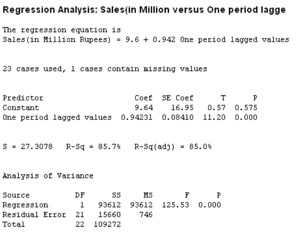
Sales ![]()
Projected sales for 2006 ![]()
= 113.22 million rupees
Projected sales for 2007 ![]()
= 116.25 million rupees
Self-Practice Problems
20C1. Hindustan Copper Ltd was incorporated in 1967 to take over the plants and mines at Rajasthan and Jharkhand from National Development Corporation Limited. Subsequently, it merged with Copper Corporation Limited. The company is engaged in activities ranging from mining, benefication, smelting, refining and production of cathodes, wire bars, and continuous cast rods.1 The following table provides the income of Hindustan Copper Ltd in different quarters from 2002–2006. Use Minitab to deseasonalize and detrend the data and forecast income of the next 6 quarters.
Source: Prowess (V. 3.1), Centre for Monitoring Indian Economy Pvt. Ltd, Mumbai, accessed December 2008, reproduced with permission.
20C2. Reckitt Benckiser (India) Ltd, formerly known as Reckitt and Coleman is a subsidiary of Reckitt Benckiser Plc. The company is engaged in the manufacture and marketing of several consumer products in many segments such household care, toiletories, laundry products, and over-the-counter pharmaceutical products.1 The table below shows the profit after tax of Reckitt Benckiser (India) Ltd in million rupees. Fit a first order, second order, and third-order autoregressive model. Test the significance of first order, second order, and third-order autoregressive parameters by using α = 0.05 Discuss which autoregressive model is appropriate for prediction. With the help of the appropriate autoregressive model, predict the profit after tax of the years 2007–2008, 2008–2009, and 2009–2010.
Source: Prowess (V. 3.1), Centre for Monitoring Indian Economy Pvt. Ltd, Mumbai, accessed December 2008 reproduced with permission.
Summary
Forecasting is a technique that can aid in future planning. Time series is an important tool for prediction. In general, there are two common ways of forecasting. These are: qualitative forecasting and quantitative forecasting techniques. Executive opinion, panel judgement, delphi methods, marketing research, and past analogy methods are some of the important methods of qualitative forecasting. Quantitative method of forecasting can be broadly divided into two categories: time series analysis and causal analysis.
The arrangement of statistical data in accordance with the occurrence of time or the arrangement of data in chronological order is known as time series. Generally in a long time series, four components are found to be present: (1) secular trend or long term movements (2) seasonal variations (3) cyclic variations, and (4) random or irregular movements. Time series methods can be broadly classified into three categories: freehand method, average methods, and exponential smoothing methods. In the freehand method, a smooth curve is obtained by plotting the values yi against time i. There are mainly three methods of smoothing through averages: moving averages method, weighted moving average method, and semi-averages method. In the moving averages method, equal weights are assigned to all the time periods whereas in the weighed moving average method, some time periods are weighed differently as compared to others. In the semi-averages method, data is divided into two equal parts with respect to time.
Exponential smoothing method weigh data from previous time period with exponentially decreasing importance in the forecast. Single exponential smoothing does not incorporate trend and seasonal components of a time series data. Holt’s double smoothing method is an exponential smoothing method, which considers trend effects in forecasting.
In time series regression trend analysis, dependent variable y is the value being forecasted and x is the independent variable time. Several methods of trend fit can be explored with a time series data. This book focuses on two methods: linear trend model and quadratic trend model. Simple linear regression is based on the slope–intercept equation of a line whereas quadratic relationship between two variables can be analysed by applying quadratic regression model.
For long run forecasts, trend analysis may be an adequate technique. However for short run forecasting, awareness about the seasonal effect on time series data is of paramount importance. Once these seasonal patterns are identified, these can be eliminated from the time series data, in order to analyse the impact of other components on time series data. This process of eliminating the seasonal effect from the time series data is referred to as deseasonalization. One of the widely used techniques to eliminate the effect of seasonality is decomposition. The decomposition technique is based on the multiplicative model concept in time series analysis. In order to eliminate the seasonal variations from the data, this chapter describes a widely used technique referred to as ratio-to- moving average method.
Autocorrelation is a problem that occurs when data is regressed . When error terms of a regression model are correlated, autocorrelation occurs. Autoregression is a forecasting technique, which takes into account the advantage of the relationship of the value (yi) to the previous values (yi –1, yi –2, yi –3…).
Key terms
Additive model, 518
Autocorrelation, 544
Autoregression, 546
Cyclic variations, 516
Decomposition, 518
Delphi method, 514
Deseasonalization, 537
Double smoothing method, 549
Executive opinion method, 514
Exponential smoothing
method, 526
Freehand method, 521
Irregular variations, 518
Marketing research method, 515
Moving average method, 537
Multiplicative model, 518
Panel judgement method, 514
Past analogy, 514
Qualitative methods of
forecasting, 514
Seasonal Variations, 516
Secular trend, 516
Single exponential smoothing, 530
Time Series, 514
Notes
1. Prowess (V. 3.1), Centre for Monitoring Indian Economy Pvt. Ltd, Mumbai, accessed September 2008, reproduced with permission.
2. http://www.hindwarebathrooms.com, accessed September 2008.
Discussion Questions
1. What are the various methods of forecasting?
2. Explain qualitative and quantitative methods of forecasting.
3. What are the various components of a time series?
4. Explain additive and multiplicative models of time series.
5. Describe the methods use to measure errors in forecasting.
6. Explain the concept of freehand method, average method, and exponential smoothing method.
7. Explain the concept and application of the double exponential smoothing method. Also explain the concept of double exponential smoothing using Holt’s method.
8. Explain the regression method of forecasting with special reference to two methods: linear trend model and quadratic trend model.
9. What is the process of obtaining deseasonalized data from a time series? Also explain the method of obtaining de-seasonalized and detrended values.
10. Explain the concept of autocorrelation and autoregression. How can the concept of autoregression be used in fore-casting?
Numerical Problems
1. The following table provides the travelling expenses incurred by the sales executive of a company from 1993 to 2004. Prepare a time series plot with these figures.
2. Compute a 3-yearly moving average for the data given in Problem 1.
3. Compute a four yearly moving average for the data given in Problem 1.
4. Determine the straight line trend by semi-averages method for the following time series data related to the sales of a cement manufacturing company. Also determine the projected sales for 2008.
5. The following table provides the number of units produced by a calculator manufacturer in different years.
Use exponential smoothing method with α = 0.3; α = 0.5, and α = 0.7 to forecast the production of calculators.
6. Use exponential smoothing method with α = 0.2; α = 0.5, and α = 0.8 to forecast the sales of a company. The sales values for 14 years are given in the table below:
7. The following table lists the number of units manufactured by a company in 12 years. Fit a straight line trend by the method of least squares and estimate the sales in 2010.
8. The following table lists the sales values of a company for five years for all the four quarters of the year. Calculate the seasonal indexes. In addition, detrend and deseasonalize the data and obtain the projected values after deseasonalization and detrending.
Case Study
Case 20: Nicholas Piramal India Ltd: Success Through Innovation
Introduction: An Overview of the Domestic Pharmaceutical Market
The domestic pharmaceutical market has witnessed high growth as a result of rising income levels and increasing penetration of modern medicine. As per the ORG-IMS MAT report for March 2008, the growth for the financial year 2007–2008 was 14.8%. Chronic therapies continue to grow faster than acute. The domestic pharmaceutical industry is centered on branded generics and is intensely competitive. The top 10 companies account for only 36% of the market share. Pharmaceutical industry continues to be highly fragmented with has more than 20,000 registered units.1 The industry expanded drastically in the last two decades. The leading 250 pharmaceutical companies control 70% of the market with the market leader holding nearly 7% of the market share.2 The demand for drug and pharmaceuticals is estimated to be ![]() 1675 billion by 2014–2015.3
1675 billion by 2014–2015.3
Nicholas Piramal India Ltd: India’s Second Largest Pharmaceutical Healthcare Company
Nicholas Piramal India Ltd is India’s second largest pharmaceutical healthcare company and is a leader in the cardio-vascular segment. The company came into existence after its acquisition of Nicholas Laboratories from Sara Lee in 1988. It has a strong presence in the antibiotics and respiratory segment, pain management, neuro-psychiatry, and anti-diabetis segments. The company has also made forays into biotechnology in key therapeutic areas for which it has formed several global alliances. Nicholas Piramal India Ltd is a part of the USD 500 million Piramal Enterprises (PIL), which is one of India’s largest diversified business houses.4
Rebranding Exercise at Nicholas Piramal
Nicholas Piramal has worked out a complex internal rebranding exercise for creating a common brand identity across its various divisions such as Wellquest (clinical trials division), Wellspring (pathlabs), and Actics. The company wants to adopt a common name and a new logo that can be easily identified by its clients across businesses. Discussing this exercise, Swati Piramal, Director, Strategic Alliance and Communications, NPIL told Financial Express in January 2008, “Yes, we have been discussing a common brand identity, including a change in the company logo. This is an effort to rationalize the various entities and for the ease of the regulatory process.5” As a result of this exercise in April 2008, Nicholas Piramal India Ltd Chairman Ajay Piramal announced, “It has been a decade since Nicholas Piramal India Ltd was established. There was no association of Nicholas in Nicholas Piramal India Ltd and moreover it was the name of a multinational. With the emergence of India globally, Nicholas lost its relevance, so we have decided to rechristen the company as Piramal Healthcare Ltd.6”
Great People Create Great Organizations
For Piramal Healthcare Ltd, its employees are vital. The belief that “great people create great organizations” has been at the core of the company’s approach to its people. It has created a favourable work environment that encourages innovation and meritocracy. It has introduced a Career Opportunity Programme (COP) to promote internal talent. The learning and development cell of the company is dedicated to developing managerial skills and inspiring them to grow as business leaders. The company has also invested in enhancing the size of the sales. As a result, during the financial year 2007–2008, it increased its sales force from 3154 people to 3789 people.1
Table 20.01 lists the sales figures of the company from 1990 to 2007:
TABLE 20.01 Sales of Nicholas Piramal India Ltd from 1990–2007
Source: Prowess (V. 3.1), Centre for Monitoring Indian Economy Pvt. Ltd, Mumbai, accessed September 2008, reproduced with permission.
1. Prepare a time series plot with the help of the data given in Table 20.01.
2. Compute a 3-year-moving average for this time series.
3. Use exponential smoothing method with α = 0.3; α = 0.5 to forecast sales.
4. Use Holt’s two parameter (α = 0.3, β = 0.5) method to forecast sales.
Notes
1. Prowess (V. 3.1), Centre for Monitoring Indian Economy Pvt. Ltd. Mumbai, accessed September 2008, reproduced with permission.
2. www.pharmaceutical-drug-manufactures.com/pharmacu-itical-industry/, accessed September 2008.
3. http://wwwindiastat.com, accessed September 2008, reproduced with permission.
4. www.nicholaspiramal.com/media_companyprofile. htm, accessed September 2008.
5. www.financialexpress.com/news/Nicholas-Piramal-joins-rebranding-jitterbug/257357, accessed September 2008.
6. www.expressindia.com/latest-news/nicholas- piramal-rechristened-piramal-healthcare/293233/, accessed September 2008.