Chapter 10

Descriptive Statistics: Measures of Central Tendency

Learning Objectives

Upon completion of this chapter, you will be able to:

• Understand the concept of arithmetic mean, geometric mean, harmonic mean, median, mode, quartiles, percentiles, and deciles
• Compute arithmetic mean, geometric mean, harmonic mean, median, mode, quartiles, percentiles, and deciles
• Use MS Excel, Minitab, and SPSS for computing mathematical averages, positional averages, and partitional values

10.1 Introduction

This chapter focuses on the measures of central tendency, and Chapter 11 discusses the measures of dispersion and shape. After the classification and tabulation of data, we need to use a few measures that can reveal the basic features of the data. In statistics, a tool which represents the basic features of data is referred to as an “average.” An average value is a single value that describes an entire group of values. In other words, it is a single value within the range of the data that is used to represent all the values in the series. Simply speaking, the average of a statistical series is the value of the variable which is representative of the entire series.

10.2 Central Tendency

A central tendency is a single value which is used to represent an entire set of data. It is a typical value around which most of the other values cluster. In other words, the tendency of the observations to concentrate around a central point is known as central tendency.

10.3 Measures of Central Tendency

Statistical measures that indicate the location or position of a central value to describe the central tendency of the entire data are called the measures of central tendency. In statistics, there are various types of measures of central tendency, some of which can be broadly classified as follows:

1. Mathematical Averages
   1. (a) Arithmetic mean or mean
      • Simple
      • Weighted
   2. (b) Geometric mean
   3. (c) Harmonic mean
2. 2. Positional Averages
   1. (a) Median
   2. (b) Mode
   3. (c) Quartiles
   4. (d) Deciles
   5. (e) Percentiles

An average should possess some basic prerequisites. A brief description of these prerequisites is given below.

10.4 Prerequisites for an Ideal Measure of Central Tendency

Some important characteristics of an ideal measure of central tendency are as follows:

1. It should be rigidly defined.
2. It should be readily comprehensible and easy to calculate.
3. It should be based upon all the observations.
4. It should be suitable for further mathematical treatment.
5. It should be affected as little as possible by the fluctuations of sampling.

There are various measures of central tendency of data. The most common and widely used measure is the arithmetic mean. The following section discusses various mathematical averages and their computation.

10.5 Mathematical averages

Methods of computing mathematical averages are classified according to the nature of the data. In classification and tabulation of data, values of the observations can be arranged in any of the ­following series:

1. Individual series or ungrouped data
2. Discrete frequency distribution
3. Continuous frequency distribution

Computation of mathematical averages can also be differentiated according to the nature of the data series. The data series could be in the form of individual series, discrete frequency distribution, or continuous frequency distribution. It is important to note that individual series comprises of raw (ungrouped) data. Discrete frequency distribution and continuous frequency distribution comprise of grouped data. In discrete frequency distribution, the raw data is grouped with frequencies, whereas in continuous frequency distribution; the raw data is grouped with frequencies and class intervals.

10.5.1 Arithmetic Mean

The arithmetic mean (AM) of a set of observations is their sum, divided by the number of observations. It is generally denoted by or AM. Population mean is denoted by m. Therefore,

Arithmetic mean is of two types:

• Simple arithmetic mean
• Weighted arithmetic mean

10.5.1.1 Calculation of Simple Arithmetic Mean

Arithmetic mean can be computed differently for three different types of series. In other words, arithmetic mean can be computed differently for individual series, discrete frequency distribution, and continuous frequency distribution.

Computation of arithmetic mean for individual series

The arithmetic mean of an individual series can be calculated by dividing the sum of the observations by the number of observations.

In a series x₁, x₂, x₃,… x_n, the arithmetic mean can be calculated by

To understand the procedure of computing arithmetic mean for an individual series, see Example 10.1.

Example 10.1

A rainwear manufacturing company wants to launch some new products in a new state. The rainfall in the state (in cm) for the past 10 years is given in Table 10.2. Find the average rainfall of the state in the past 10 years.

TABLE 10.2 Rainfall for 10 years (1995–2004)

Soultion

For computing average rainfall, we have to first compute the total rainfall in 10 years (see Table 10.3) and then divide this total by the total number of years, 10.

TABLE 10.3 Total rainfall in ten years

 

Hence, the average rainfall in 10 years in the state is 148.5 cm.

Computation of arithmetic mean for discrete frequency distribution

In this type of distribution, every term is multiplied by its corresponding frequency and the total sum of these products is divided by the sum of frequencies. Hence, for a given series x₁, x₂, x₃, …, x_n, with corresponding frequencies f₁, f₂, f₃, …, f_n, the arithmetic mean AM is given by

To understand the method of calculating the arithmetic mean for a discrete series, see Example 10.2.

Example 10.2

The weekly earnings of 187 employees of a company is given in Table 10.4. Find the mean of the weekly earnings.

Soultion

In a discrete series, each value must be multiplied by its frequency. The next step is to divide the sum of this product by the total sum of the frequencies to arrive at the arithmetic mean (see Table 10.5).

TABLE 10.5 Product of the weekly earnings and number of employees

 

AM

Hence, the average weekly earning is 88.55.

Computation of arithmetic mean for continuous frequency distribution

The process of computing arithmetic mean for a continuous frequency distribution is the same as the process of computing arithmetic mean for a discrete series. In a continuous ­frequency distribution, the class intervals are given. We take the midpoint of each class interval as the value of x. The remaining steps are the same as that for computing the arithmetic mean of a discrete series. The formula given below is used for computing the arithmetic mean for a continuous series:

Example 10.3 explains the procedure of computing arithmetic mean for continuous frequency distribution.

Example 10.3

From Table 10.6, find the arithmetic mean.

TABLE 10.6 Data related to class intervals and frequencies

 

Soultion

For computing arithmetic mean in a continuous frequency distribution, we need to compute the midpoint of class intervals (x). The midpoints are multiplied by the corresponding frequencies (fx). The sum of this product is obtained and is divided by the sum of frequencies (Table 10.7).

Table 10.7 Data given in Table 10.6 arranged with class midpoint, frequencies, and the product of mid-points and frequencies

 

10.5.2 Mathematical Properties of Arithmetic Mean

The arithmetic mean is based on all the observations and is capable of further mathematical treatment. It has some very important mathematical properties:

1. The sum of the deviations of the items from the arithmetic mean is always zero, that is, . This property is well explained by Table 10.8:

   here,

   

   So, Σ(x_i – = 0 (from Table 10.8)

2. The sum of the squares of the deviation of a set of values is minimum when taken from the mean.

   To understand this property, see Table 10.9. The sum of the squares of the deviation from mean (computed as 30) can be computed as in Table 10.9.

   TABLE 10.8 Sum of the deviations of the items from the arithmetic mean

   

   TABLE 10.9 Sum of the squares of the deviation from mean

   

   The sum of the squares of the deviation of a set of values is minimum when taken from the mean.

   In this case, the sum of the squares of the deviation is equal to 1000. If the deviation would be taken from any other value, say 20, then the sum of the squares of the deviations would be greater than 1000 as shown in Table 10.10.

   TABLE 10.10 Sum of the squares of the deviation from any value other than mean

   

   It is clear that when the sum of the square was taken from the arithmetic mean, it was 1000 and when it was taken from any other value, for example, 20 as in Table 10.10, it was 1500, which is greater than 1000. This result can be generalized.

3. Simple arithmetic means may be combined to form a composite mean. The formula for com posite mean is

   

   Simple arithmetic means may be combined to form a composite mean.

10.5.3 Merits and Demerits of Arithmetic Mean

No mathematical or positional average is free from merits and demerits. It is important to understand its merits and demerits to have an idea about its appropriate application. Some of the merits and demerits of arithmetic mean are listed below.

10.5.3.1 Merits

1. It is rigidly defined.
2. It is easy to calculate and understand.
3. It is based upon all the observations.
4. It is capable of further algebraic treatment.
5. Arrangement of data in ascending or descending order is not necessary.
6. Of all the averages, arithmetic mean is the least affected by fluctuations of sampling.

10.5.3.2 Demerits

1. It is highly affected by extreme values.
2. It cannot be determined by inspection.
3. When dealing with qualitative characteristics, such as intelligence, honesty, beauty, etc. arithmetic mean cannot be used. In such cases, median can be used.
4. In extremely asymmetrical (skewed) distributions, the arithmetic mean is not a suitable measure.

10.5.4 Weighted Arithmetic Mean

In the computation of arithmetic mean, equal importance is given to all the items of a series. However, there are cases where all the items are not of equal importance, and importance itself is relative by nature. In other words, some items of a series are more important as compared to the other items in the same series. In such cases, it becomes important to assign different weights to different items. The weighted mean can be used to calculate an average that takes into account the importance of each value with respect to the overall total. For example, to get an idea of the change in the cost of living of a certain group of people, a simple mean of the prices of the commodities consumed by them will not be an appropriate tool for measuring average price, as all the commodities may not be of equal importance. For example, wheat, rice, and pulses may be more important when compared with cigarettes, tea, and other luxury items.

10.5.4.1 Computation of Weighted Mean

The formula for calculating weighted mean is

where x is the value of the item and w the weights attached to the corresponding items.

Self-Practice Problems

10A1. Determine the mean from the following ­series:

23 27 28 25 20 21 34 18 29 21 16

10A2. Determine the mean from the following frequency ­distribution:

10A3. Determine the mean from the following class intervals:

10A4. The following data shows the consumption of primary sources of conventional energy in India from 1996–1997 to 2005–2006. This includes coal, crude petroleum, natural gas, and electricity. Compute the average consumption of coal, crude petroleum, natural gas, and electricity from 1996–1997 to 2005–2006.

10A5. IDBI Bank Ltd was incorporated under an act of Parliament in 1964 as a wholly owned subsidiary of the Reserve Bank of India. The main purpose of this move was to monitor and coordinate the activities of financial institutions at the state and national level. IDBI Bank has many products and is mainly involved in providing long-term finance for various projects. The income of IDBI Bank from 1998–1999 to 2006–2007 except 2003–2004 is given below. Compute the average income of the bank from 1998–1999 to 2006–2007(Except 2003–2004).

10A6. Find the arithmetic mean from the following data:

10.5.5 Geometric Mean

Geometric mean (GM) is the nth root of the product of n items of a series. For example, if there are three items in a series, their geometric mean would be the cube root of the product of all the three items. If these three items are 4, 6, and 9, then their geometric mean, which is generally denoted by G, can be computed as

In the previous sections, we have seen that average can be calculated differently for various types of distributions. Likewise, geometric mean can also be calculated for three different types of series. These are

1. individual series or ungrouped data;
2. discrete frequency distribution; and
3. continuous frequency distribution.

In the following section, we discuss the computation of geometric mean for these three types of distributions.

10.5.5.1 Computation of Geometric Mean for Individual Series

Suppose an individual series contains n items as x₁, x₂, x₃, … , x_n. Then, geometric mean G is defined as

Taking logarithms on both sides of the above equation, we have

log G =

log G =

G = antilog

Example 10.4

The annual rate of growth for a factory for 5 years is 7%, 8%, 4%, 6% and 10% respectively. What is the average rate of growth per annum for this period?

Soultion

If the growth in the beginning is 100, then for 5 years, the growth is as given in Table 10.11.

TABLE 10.11 Computation of Geometric mean for Example 10.4

G = antilog

= antilog

= antilog (2.0293)

= 106.98

The required average growth rate is 106.98 – 100 = 6.98. Therefore, the average rate of growth percentage per annum is 6.98%.

 

10.5.5.2 Geometric Mean for Discrete and Continuous Series

If there are n items in a discrete series, x₁, x₂, x₃, …, x_n, with f₁, f₂, f₃, …, f_n, frequencies, respectively, then N can be defined as the sum of all frequencies, that is, N = f₁ + f₂ + f₃ +…+ f_n. Then, geometric mean G is given by

Taking logarithms on both sides in the above equation, we have

The above formula can be used for calculating the geometric mean for a discrete frequency distribution. So, geometric mean for a discrete frequency distribution can be obtained by inserting one more column in the solution (as compared to computing geometric mean for an individual series), that is . Similarly the geometric mean for a continuous series can be obtained by finding out the mid-value of the interval, in the usual way. Practically, geometric mean is widely used for calculating the average rate of growth. For large data sizes, geometric mean can be used to calculate the average rate of growth or depreciation.

10.5.6 Average Rate of Growth

As mentioned earlier, geometric mean is commonly used for the calculation of the average rate of growth. For the same purpose, the following formula is used.

P_n = P₀ (1 + r)ⁿ

where P_n is the figure at the end of period n, P₀ is the figure at the beginning of the period, r is the average rate of change, and n the length of the period.

Taking logarithms on both the sides of the above equation, we obtain

Example 10.5

The population of a country increased from 360 million to 380 million from 1991 to 1995. Find the average annual growth rate of population.

Soultion

The formula for calculating the average annual growth rate is

log (1 + r) =

1 + r = antilog

- 1

= (1.0135–1)

= 0.0135

= 1.35%

Hence, the annual growth rate of the population is 1.35%.

10.5.7 Importance of Geometric Mean

We have already studied how the arithmetic mean can be used as a tool for obtaining averages. But what could be the use of geometric mean? What is the need to use geometric mean as an average tool as we already have averages of various types? The answer lies in the fact that geometric mean is generally used in situations where small items are assigned large weights and vice versa. The following are some of the special uses of geometric mean.

1. Geometric mean is useful for calculating the average percentage increase or decrease.
2. In the construction of index numbers, geometric mean is considered to be the best average tool.

Example 10.6 explains the special use of geometric mean as a tool of computing average percentage increase.

Example 10.6

The price of a commodity increased by 8% from 1993 to 1994, 12% from 1994 to 1995, and 76% from 1995 to 1996. The average price increase from 1994 to 1996 is quoted as 28.64% and not 32%. Explain and verify the result.

Soultion

Here, the average of the percentage increase over a period of 3 years is to be computed. Thus, geometric mean is the most appropriate average tool. The appropriateness of using geometric mean can also be checked by first computing the average of the growth and then by verifying the result. The arithmetic mean of the percentage increases is

However, an average increase of 32% is not the correct answer (as was clarified in the verification part). To obtain the correct answer, the GM of the percentage increase is to be computed (Table 10.12).

 

Therefore, the average increase from 1994 to 1996 is 128.64266 – 100 = 28.64266%. Now, we verify the actual situation (Case 1) by comparing it with the situation where the average increase is 32% (arithmetic average, Case 2), and when the average increase is 28.64266% (geometric mean, Case 3).

Verification

Case 1: When the commodity price increases by 8% from 1993 to 1994, 12% from 1994 to 1995 and 76% from 1995 to 1996 (Table 10.13).

 

Case 2: When the average increase is 32% (arithmetic mean) per year (Table 10.14).

 

Case 3: When average increase is 28.64266% (geometric mean) per year (Table 10.15)

 

From Tables 10.13–10.15, it can be seen very easily that in Cases 1 and 3, the price level at the end of the third year is the same. Hence, geometric mean is an appropriate tool of computing average percentage increase.

10.5.8 Merits and Demerits of Geometric Mean

In situations where the average rate of change has to be calculated over a period of several years the use of arithmetic mean leads to a faulty result (as discussed earlier). In such cases, the geometric mean has been found to be an appropriate tool. However, this does not mean that this average tool is free from limitations. The following are some of the merits and demerits of geometric mean.

10.5.8.1 Merits

1. It is rigidly defined.
2. It is useful in dealing with ratios and percentages and can be very well used in determining the rate of increase or decrease.
3. It is suitable for algebraic treatments. If GM₁ and GM₂ are geometric means of two series and n₁ and n₂ are the number of observations of these two series, respectively, then the combined geometric mean can be easily calculated by applying the formula
4. Some statistical errors such as fluctuation of sampling have the least effect on it.
5. It is based on all the observations.

10.5.8.2 Demerits

1. It is difficult to compute and understand, therefore, its application is limited.
2. For negative and zero values in a series, it is difficult to apply.

SELF-PRACTICE PROBLEMS

1. 10B1. Compute the geometric mean for the following series.

23 25 32 36 39 41 43 21 47 43

10B2. A firm purchased an old machine for its manufacturing process. The seller claims that the machine will depreciate 40% in the first year, 30% in the second year, 25% in the third year, and 20% in the fourth year. Compute the average depreciation for all 4 years?

10B3. A detergent company launched a new product in the market in 2001–2002 and planned for massive advertisements to promote the product in the market. The percentage increase in sales from 2003–2004 to 2007–2008 is given below. Compute the average percentage increase in sales from 2003–2004 to 2007–2008.

10B4. The following data gives the production of wheat (in million tonnes) along with percentage coverage under irrigation in India from 1982–1983 to 2003–2004. Calculate the average production of wheat from 1982–1983 to 1992–1993 and 1993–1994 to 2003–2004. Also compute the average percentage coverage under irrigation from 1982–1983 to 1992–1993 and 1993–1994 to 2003–2004.

10.5.9 Harmonic Mean

The harmonic mean of any series is the reciprocal of the arithmetic mean of the reciprocal of the variate, that is, the harmonic mean by definition is given by

= Arithmetic mean of

=

=

Like any other measure of central tendency, harmonic mean can also be calculated in three different ways for three types of distributions. In the following section, we discuss how to compute the harmonic mean for

1. an individual series;
2. a discrete frequency distribution; and
3. a continuous frequency distribution.

10.5.9.1 Computation of Harmonic Mean for Individual Series

For a series like x₁, x₂, x₃, …, x_n, the harmonic mean is given by

=

=

Example 10.7

Calculate the harmonic mean of the following items:

2.0, 1.5, 3.0, 10.0, 250.0, 0.5, 0.905, 0.095, 2000, 0.099

Soultion

To compute harmonic mean, we have to first compute the reciprocals of each item as given in Table 10.16.

HM = Reciprocal of

= Reciprocal (2.53367)

= 0.39468

10.5.9.2 Computation of Harmonic Mean for Discrete Frequency Distribution and Continuous Frequency Distribution

For a discrete frequency distribution, frequencies are also given with individual values. So, for a discrete frequency distribution, the formula includes these frequencies and takes the form

=

or H =

where

In the case of a continuous series, the same formula can be applied and the mid-values of the classes are taken as x_is. Example 10.8 clarifies the procedure for calculating the geometric mean and harmonic mean for a continuous series.

Example 10.8

Table 10.17 shows the salary ranges (in thousand rupees) and the number of employees for a manufacturing firm.

Example 10.10

Calculate AM, GM, and HM for the observations 2, 4, 8, 12, and 16, and show that AM > GM > HM.

Soultion

GM = antilog

= antilog

= antilog

GM = antilog = 6.575

HM =

=

= 4.89

Thus, we can see that AM > GM > HM.

Example 10.11

The AM of two numbers is 10; the GM of these numbers is 8. Find the HM of these numbers.

Soultion

We know that

(GM)² = (AM) × (HM)

8² = 10 × HM

HM =

10.5.13 Merits and Demerits of Harmonic Mean

Although harmonic mean is based upon all the observations and gives weightage to smaller values, its application is limited because of its shortcomings. It is useful in cases where small items need to be given very high weightage. The following are some of the merits and demerits of harmonic mean.

10.5.13.1 Merits

1. It is based on all the observations.
2. It is suitable for algebraic treatment.
3. It gives more importance to smaller values.

10.5.13.2 Demerits

1. It is difficult to compute.
2. When there are positive and negative values in a series or when one or more items are zero, then it is difficult to compute.
3. It gives more importance to smaller values. This merit of harmonic mean is a demerit in itself. This property of harmonic mean becomes a hindrance in its wide use with regard to economical data.

Self-Practice Problems

10C1. Compute the harmonic mean from the following data series:

4.0; 3.5; 5.0; 11.0; 340.0; 0.8; 0.804; 0.040; 5000; 0.088.

10C2. Compute the harmonic mean from the following distribution:

10.6 POSITIONAL AVERAGES

Arithmetic mean, geometric mean, and harmonic mean are all mathematical in nature and are measures of quantitative characteristics of data. To measure the qualitative characteristics of data, other measures of central tendency, namely median and mode are used. Positional averages, as the name indicates, mainly focus on the position of the value of an observation in the data set.

10.6.1 Median

The median of a distribution is the value of the variable that divides it into two equal parts so that one half of the data has values less than the median while the other half has values greater than the median. Median may be defined as the middle or central value of the variable when values are arranged in the order of magnitude. In other words, median is defined as that value of the variable that divides the group into two equal parts, one part comprising all values greater and the other all values lesser than the median.

10.6.2 Calculation of Median

As discussed earlier (Section 10.5), the calculation of median can also be broadly classified into three categories:

1. Median for the individual series.
2. Median for the discrete frequency distribution.
3. Median for the continuous frequency distribution.

10.6.2.1 Computation of Median for the Individual Series

In this type of distribution, data can be arranged in ascending or descending order. If there are n terms (observations) in the data, there can be two cases:

Case 1: If n (number of observations) is odd, then the middle term of the series is the th term and is the value of the median.

Case 2: If n (number of observations) is even, then there will be two middle terms. These will be the term and term. In this case, the arithmetic mean of their value will be considered to be the value of the median.

The following two examples are based on Case 1 (Example 10.12) and Case 2 (Example 10.13) for computing median.

Example 10.12

The consumption of printing paper reams (in units) for the first 11 months of a computer operator is given as

10, 11, 12, 15, 18, 22, 8, 10, 12, 15, 25

Find the median.

Soultion

By arranging the data in ascending order, we get the series

8, 10, 10, 11, 12, 12, 15, 15, 18, 22, 25

The number of terms in this series is 11 which is odd.

Hence, the required median (M_d) = value of the observation

= value of the 6th observation = 12.

Example 10.13

Table 10.21 relates to the monthly salaries of employees (in thousand rupees). Compute the median salary of the employees.

Soultion

To compute the median, we first arrange the data in ascending order.

120, 128, 132, 135, 136, 138, 148, 150, 151, 153

This data series contains 10 items. As the number of observations in this data series is even, median will be the average of term and term, that is, average of term and term. Hence, median will be the average of the 5th and 6th term.

So, median is

Thus, the median salary is 37,000.

10.6.2.2 Computation of Median for a Discrete Frequency Distribution

In the case of a discrete series, median can be calculated by using the following steps:

1. Arrange the data in ascending or descending order of magnitude.
2. Obtain cumulative frequencies.
3. Size of item must be determined, when N is the total of all the frequency, that is, .
4. The value for which cumulative frequency includes item is taken as the median.

Example 10.14

Calculate the median for the values and frequencies given in Table 10.22.

Soultion

As a first step we calculate the cumulative frequencies (as shown in Table 10.23).

Size of item = item = 47.5

 

Median is the value for which cumulative frequency includes 47.5th value. Cumulative frequency 51 of value 7 includes 47.5th value. Hence the median is 7.

10.6.2.3 Determination of Median for a Continuous Frequency Distribution

As in a discrete frequency distribution, in case of a continuous series also cumulative frequencies are calculated. As a next step the size of N/2th item is computed (N being the total frequency). Then, the median class in the cumulative frequencies column where the size of N/2th item falls is located. Then, the following formula is applied to calculate median:

Median =

where l is the lower limit of the median class, N the sum of the frequencies, c the cumulative frequency of the class preceding the median class, and i the width of the median class.

Note that in the case of a continuous frequency distribution, the size of N/2th item is to be computed. In the case of individual series and discrete frequency distribution, size of the item was computed because we wanted to compute specific items or individual values that divides the data into two equal parts. In the case of a continuous frequency distribution, however, the individuality of frequencies is lost and we try to find out a specific point in the curve that divides it into two equal parts (half of the frequencies are on the one side the curve and half the frequencies on the other side of the curve). N/2 divides the curve area into two equal parts, not . Hence, we use instead of for the computation of median in a continuous frequency distribution.

Example 10.15

Delta Tiers employed 159 employees for a factory located at Kanpur. The company’s management is worried about the high absenteeism rate in the organization. Before taking any corrective action, the management has decided to calculate the median leaves availed by the employees. Table 10.24 shows vacations availed in a year and the number of employees who availed vacations. Compute median from the data.

Soultion

For computing the median, for a continuous frequency distribution we have to compute cumulative frequencies as shown in Table 10.25.

 

Here N = 159, which is an odd number.

which falls in the class 30–40 (see the row of the cumulative frequency 95 which contains 79.5). Hence the median class is 30–40.

l = lower limit of median class = 30

f = frequency of median class = 45

c = total of all frequencies preceding median class = 50

i = width of class interval of median class = 10

Median

= 30

= 30

= 30 = 36.55

10.6.3 Merits and Demerits of Median

Median has several advantages over mean. More importantly, as compared to arithmetic mean, median is the least affected by extreme values. The following is a list of merits and demerits of median.

10.6.3.1 Merits

1. It is well defined, and based on all observations. Therefore, it can be easily ­ computed.
2. Extreme values do not affect the median as strongly as the mean.
3. Median can be computed even when data is of qualitative nature such as colour, honesty, beauty, etc.

10.6.3.2 Demerits

1. As median is a positional average, data must be arranged in order before any calculation can be performed.
2. Median computation can be time-consuming for any data set with a large number of elements.
3. It is not suitable for algebraic treatment.
4. Sometimes it may not be a true representative of data.

Self-Practice Problems

10D1. Compute the median for the series given in Problem 10A1.

10D2. Compute the median for the series given in Problem 10A2.

10D3. ICICI Bank is a key bank in India with a solid international presence. In May 2002, it merged with Industrial Credit Investment Corporation of India Limited (ICICI Ltd). Later two more companies, ICICI Personal Financial Services and ICICI Capital Services, came under the umbrella of the merged entity. After the merger ICICI Bank became the second largest bank in India after State Bank of India. The following data gives the quarterly income figures of ICICI Bank from March 2003 to March 2007. Compute the mean and median from the income figures.

10D4. TVS Srichakra is one of India’s leading two- and three-wheeler tyre manufacturing companies. The growth in the automobile industry has contributed to a growth in the tyre industry. The following data depicts the quarterly net sales of TVS Srichakra from June 1998 to March 2007. Find the average net sales and median net sales from the data.

10D5. An insurance company obtained the following data for accident claims from a particular region. Obtain the median from this data.

10.6.4 Mode

Mode is defined as the value that is repeated most often in the data set. It is the value of the variate having the maximum frequency in a data series. The mode of a distribution is the value at the point around which the items tend to be most heavily concentrated. In other words, the value of the variable which occurs most frequently in a distribution is called the mode.

In a distribution, there may be one, two, or more than two modes. A distribution which has a single mode is called unimodal distribution and a distribution which has two modes is called a bimodal distribution (Figures 10.1 and 10.2).

FIGURE 10.1 Unimodal distribution

FIGURE 10.2 Bimodal distribution with two unequal modes

For a frequency distribution, for which a curve is drawn, the mode is the value of the variable at which the curve reaches its peak or maximum. In a bimodal distribution, we can observe two peaks or two maximum points, which state that these points are higher than the neighbouring values in terms of frequencies with which they are observed. Figures 10.1 and 10.2 exhibit unimodal and bimodal distributions.

The concept of a mode is widely used in production. For example, a shoe manufacturer will produce shoes of a size that will fit the maximum number of customers. A customer who has a large shoe size, say size 11, may find it difficult to buy a shoe that fits him.

Using mode as an average tool, we can overcome some drawbacks of the measures of mathematical average (arithmetic mean) and positional average (median). There are many situations in which arithmetic mean and median fail to reveal the true characteristics of data. For example, in the presence of extreme values in a data series, the arithmetic mean may not be an appropriate averaging tool. Similarly, the median may not be a true representative of data owing to the uneven nature of the distribution. As already discussed, median is the value which divides the data into two equal parts. For example, in a data series consisting of values from 0 to 1000, it is possible that the lower part of the distribution ranges from 0 to 10 and the upper part of the distribution ranges from 10 to 1000. In such a case, the median value 10 is not a true central representative of the data. Both these drawbacks of mean and median may be tackled by using mode, which is the value of the variable which occurs most frequently in a distribution.

10.6.5 Determination of Mode

Like every other method of determining various averages, mode can also be determined differently in three types of distribution: mode in an individual series, a discrete frequency distribution, and a continuous frequency distribution. As a first case, we take into consideration the mode in an individual series.

10.6.5.1 Computation of Mode for the Individual Series

In the case of an individual series, data is arranged in order and mode can be determined by inspection only. The value of the variable (in data series) which occurs the most or the value of the data series with maximum frequency is the mode of the data series. For example, for a series 1, 1, 3, 3, 3, 3, 4, 5, 8, 8, 16, 16 (arranged in the order of magnitude), observation 3 has the maximum frequency 4. Therefore, mode of the series is 3.

10.6.5.2 Computation of Mode for Discrete Frequency Distribution

By this method, mode can be determined very easily (the value with the maximum frequency), but in the case of repeated frequency distribution, irregular distribution, and in cases where maximum frequency occurs in the very beginning or at the end of the distribution, mode cannot be determined by this method. The modal value is determined by applying grouping method. The grouping method can be performed in three steps, which are (1) preparation of grouping table, (2) preparation of analysis table, and (3) finding the mode.

Preparation of grouping table

In a grouping table, normally there are six columns. If necessary more columns may be constructed. The details of these six columns are explained below:

Column 1: Original frequencies (given in the data).

Column 2: Given frequencies are added in twos and the highest total is marked.

Column 3: Leaving the first frequency, the remaining frequencies are added in twos and the highest total is marked.

Column 4: Given frequencies are added in threes and the highest total is marked.

Column 5: Leaving the first frequency, the given frequencies are added in threes.

Column 6: Leaving the first two frequencies, the given frequencies are added in threes.

The preparation of the analysis table and finding the mode are explained with the help of Example 10.16.

Example 10.16

Calculate the mode from the following series:

Soultion

Here, the maximum frequency 9 belongs to two values of the items 12 and 14. However, owing to the irregular distribution of frequencies, we use the grouping method to decide which one may be considered as the maximum frequency. The grouping table is constructed as per the steps outlined above (see Table 10.26). The analysis is explained in Table 10.27.

 

 

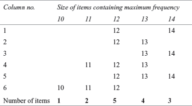
As 12 occurs the maximum number of times (5), the value 12 is the mode.

10.6.5.3 Computation of Mode for Continuous Frequency Distribution

In a continuous frequency distribution, first the modal class is determined. This can be determined either by inspection or by grouping method. The required mode lies within the limits of this modal class and is determined by the following formula:

M₀ = l +

where M₀ is the mode, l the lower limit of the modal class, f₁ the frequency of the modal class, f₀ the frequency of the class preceding the modal class, f₂ the frequency of the class succeeding the modal class, and i the width of the modal class.

The above formula is useful for exclusive and equal class intervals in ascending order. If the mode lies in the first class interval, then f₀ is taken to be zero. If the mode lies in the last class interval, then f₂ is taken to be zero.

10.6.6 Merits and Demerits of Mode

Like the other measures of central tendency, mode has its own advantages and disadvantages. It is widely used in the industry. The following are some common advantages and disadvantages of mode:

10.6.6.1 Merits

1. It is easy to understand and calculate. It can be detected by a mere look at the graph.
2. It is very useful in industries.

10.6.6.2 Demerits

1. It is not based on all the observations.
2. When data sets contain two, three, or many modes, they are difficult to interpret and compare.
3. It is neither based on all the observations nor is it suitable for algebraic treatment.

10.6.7 An Empirical Relation Between Mean, Median, and Mode

The relationship between mean, median, and mode depends upon the shape of the frequency curve; in other words, the relationship between mean, median, and mode depends upon the type of frequency distribution. For a symmetrical distribution (Figure 10.3(a)), mean, median, and mode all coincide. That is, mean = median = mode: . In the case of a negatively (left) skewed curve (­Figure 10.3(b)), mean < median < mode, that is , where as in the case of a positively skewed (right) curve (Figure 10.3(c)), mean > median > mode, that is .

FIGURE 10.3 Comparison between mean, median, and mode for (a) symmetrical, (b) negatively skewed, and (c) positively skewed distribution

For a moderately asymmetrical frequency distribution, the empirical relationship between mean, median, and mode is given by Karl Pearson and is defined as

Mode = 3(Median) – 2(Mean)

If any two values are known, the third value can be easily determined.

Self-Practice Problems

10E1. Compute the mode for the series given in Problem 10A1.

10E2. Maruti Suzuki, India’s leading company in the passenger car segment, launched various brands to cater to the diverse requirements of the Indian automobile market. In 1983, it captured the market with Maruti 800 model. It has a great national reach in terms of presence in almost all the major cities of every state in the country. The quarterly gross sales of Maruti Suzuki from December 2002 to March 2007 is given below. Compute the average, median, and mode from the table.

 

10.7 Partition values: Quartiles, Deciles, and Percentiles

Median is the value which divides the data into two equal parts. Partition values are measures that divide the data into several equal parts. There are three type of partition values: quartiles, deciles, and percentiles. Quartiles divide data into four equal parts, deciles divide data into ten equal parts, and percentiles divide data into hundred equal parts. The method of computing these partitional values is similar to the method of computing median. The only difference can be observed in terms of location of the partition value.

10.7.1 Quartiles

As discussed earlier, after arranging the data in an ordered sequence, quartiles divide the data into four equal parts using three quartiles: Q₁, Q₂, and Q₃. The first quartile is generally denoted by Q₁ and is the value for which 25% of the observations are smaller than Q₁ and 75% of the observations are larger than Q₁. The third quartile, generally denoted by Q₃, is the value for which 75% of the observations are smaller than Q₃ and 25% of the observations are larger than Q₃. The second quartile, generally denoted by the Q₂, is the value for which 50% of the observations are sma­­­­­­­­­­­­­­ller than Q₂ and 50% of the observations are larger than Q₂. Hence, the second quartile is nothing but the median. In the following section, we discuss the procedure for calculating quartiles for an individual series, a discrete frequency distribution, and a continuous frequency distribution.

10.7.1.1 First and Third Quartiles for Individual Series

For an individual series, the first and third quartiles can be computed using the following formula:

Q₁ = First quartile or lower quartile ordered observation

Q₃ = Third quartile or upper quartile ordered observation

Example 10.17

From the following data, find the first and third quartiles.

Soultion

The first and third quartiles can be computed by applying the formula discussed above. The data is already arranged in an ordered manner:

Q₁ is the size of item = size of item = size of 2nd item

Hence, Q₁ = 10

Q₃ is the size of item = size of item = size of 6th item

Hence, Q₃ = 42.

When the number of items are even in a data series, quartiles can be computed differently, as shown in Example 10.18.

Example 10.18

From the following data, find the first and third quartiles.

15 20 30 40 50 64 70 75

Soultion

Q₁ is the size of item = size of item = 2.25th value

Q₁ = 2nd value = 20 = 20 = 22.5

Q₃ is the size of item = size of item = 6.75th value

Q₃ = 6th value + 0.75(7th value − 6th value) = 64 + 0.75 (70 − 64) = 64 + 4.5 = 68.5

Hence, first quartile Q₁ = 22.5 and third quartile Q₃ = 68.5.

10.7.1.2 First and Third Quartiles for Discrete Series

The quartiles for a discrete series can also be computed using the formula discussd above. Q₁ is the size of item and Q₃ is the size of item. Here, N = Σ f.

10.7.1.3 First and Third Quartiles for Continuous Series

The first and third quartiles for a continuous series can be computed by applying the formula given below:

where l is the lower limit of the quartile class, f the frequency of the quartile class, i the class interval of the quartile class, c the total of all the frequency below the quartile class, and N the total frequency (N = Σf ).

The quartile class can be located in the cumulative frequency column, where the size of and item falls.

Example 10.19

Calculate the first and third quartiles from the data given below.

Soultion

As discussed earlier, we know that

where l is the lower limit of the quartile class, f the frequency of the quartile class, i the class interval of the quartile class, c the total of all the frequencies below the quartile class, and N the total frequency (N = Σf ).

 

Here,

Hence, lower quartile class is 10–15 (Table 10.29).

= 10 + 2.91

= 12.91

Hence, upper quartile class is 25 – 30 (Table 10.29)

= 25 + 0.83

= 25.83

So, first quartile Q₁ = 12.91 and third quartile Q₃ = 25.83.

10.7.2 Merits and Demerits of Quartiles

Quartiles are the most widely used measures of non-central locations, but they are not free from drawbacks. While calculating quartiles, the upper 25% and the lower 25% of the data remain unnoticed. However, quartiles are less affected by the presence of extreme values. Hence, quartiles possess some merits as well as some demerits. The following is a list of the merits and demerits of quartiles.

10.7.2.1 Merits

1. It is easy to calculate and simple to understand.
2. Quartiles are less affected by the presence of extreme values.

 

10.7.2.1 Demerits

1. Quartiles are not based on all the observations. In fact, 50% of the items in any series is ignored. In other words, it does not cover the first 25% and the last 25% items of a series.
2. It is not suitable for further mathematical treatment.
3. Its value is very much affected by sampling fluctuations.

10.7.3 Deciles

In a data series, when the observations are arranged in an ordered sequence, deciles divide the data into 10 equal parts. In the case of individual series and discrete frequency distribution, the general­ized formula for computing deciles is given as

where k = 1, 2, 3, …, 9 and N = Σf. Hence,

In the case of a continuous frequency distribution, the generalized formula for deciles is given as

where k = 1, 2, 3, …, 9. Other symbolic notations are as explained earlier.

10.7.4 Percentiles

In a data series, when observations are arranged in an ordered sequence, percentiles divide the data into 100 equal parts. For an individual series and a discrete frequency distribution, the generalized formula for computing percentiles is given as

where k = 1, 2, 3, …, 99 and N = Σ f. Hence,

In the case of a continuous frequency distribution, the generalized formula for computing percentiles is given as

where k = 1, 2, 3, …, 99. Other symbolic notations are as explained earlier.

Self-Practice Problems

10F1. Compute mean, median, mode, first and third quartiles, inter-quartile range, and deciles for the data given in Problem 10D3.

10F2. Compute mean, median, mode, first and third quartiles, inter-quartile range, and deciles for the data given in Problem 10D4.

10F3. Compute mean, median, mode, first and third quartiles, inter-quartile range, and deciles for the data given in Problem 10E2.

SUMMARY

A measure of central tendency is a single value which is used to represent an entire set of data. The tendency of the observations to concentrate around a central point is known as central tendency. In statistics, there are various types of measures of central tendencies, some of which may be broadly classified into two groups: mathematical averages and positional Averages. Arithmetic mean, geometric mean, and harmonic mean fall under the category of mathematical averages, and median, mode, quartiles, deciles, and percentiles belong to the category of positional averages.

The arithmetic mean of a set of observations is their sum divided by the number of observations. The weighted mean enables us to calculate an average value that takes into account the importance of each value with respect to the overall total. Geometric mean is the nth root of the product of n items of a series. Geometric mean is useful in calculating the average percentage increase or decrease. Harmonic mean of any series is the reciprocal of the arithmetic mean of the reciprocal of the variate. It has specific applications in the computation of average speed, average price, average profit, etc. under various conditions.

Arithmetic mean, geometric mean, and harmonic mean are mathematical in nature and measures of the quantitative characteristics of data. To measure the qualitative characteristics of data, other measures, namely median, mode, quartiles, and percentiles, are used.

The median of a distribution is the value of the variable which divides it into two equal parts. Mode is the value that is repeated most often in the data set. Partition values are measures of central tendencies which divide the data into several equal parts. Quartiles divide data into 4 equal parts, deciles divide the data into 10 equal parts, and percentiles divide the data into 100 equal parts.

Key terms

Arithmetic mean, 214

Central tendency, 214

Deciles, 214

Geometric mean, 214

Harmonic mean, 214

Measures of central tendency, 214

Median, 214

Mode, 214

Partition values, 243

Percentiles, 214

Positional averages, 214

Quartiles, 214

Weighted arithmetic mean, 215

 

NOTES

1. Prowess (V. 2.6), Centre for Monitoring Indian Economy Pvt Ltd, Mumbai, accessed July 2008, reproduced with permission.
2. www.ruchisoya.com/profile.htm, accessed August 2008.

Discussion questions

1. What is the meaning of measures of central tendency?
2. What are the various measures of central tendency? Describe their relative merits and demerits and their uses.
3. What are the prerequisites for an ideal measure of central tendency?
4. In light of merits and demerits of the measures of central tendency, critically examine each. Which particular measure of central tendency is considered to be the best and why?
5. Define arithmetic mean and weighted mean. Describe their application in the managerial decision-making process.
6. What is the difference between arithmetic mean and weighted arithmetic mean?
7. “Arithmetic mean is the best among all the averages” Justify this statement.
8. What is the concept of geometric mean? State its merits, demerits, uses, and its application in the decision-making process.
9. In what context is there a difference between arithmetic mean and geometric mean, and when is geometric mean useful?
10. What is the concept of harmonic mean? State its merits, demerits, uses, and application in the decision-making process.
11. State the special use of harmonic mean.
12. What is the use of various averages in management or in decision making?
13. “Each average has its own characteristics. It is difficult to say which is the best.” Discuss with suitable examples.
14. Write short notes on
    1. Arithmetic mean and weighted arithmetic mean.
    2. Median and positional averages.
    3. Mode and its application in decision making.
    4. Special use of geometric mean.
    5. Special use of harmonic mean.
    6. Relationship between the various types of averages.
15. Prepare a chart on the various types of averages and compare them on various grounds.
16. Define median, and state its merits, demerits, and use in decision making.
17. Define mode. State its merits, demerits, and its application in decision making.
18. What is the empirical relationship between arithmetic mean, median, and mode?
19. What is the meaning of partition or positional values? Write short notes on quartiles, deciles, and ­ percentiles.

Numerical problems

1. Compute the arithmetic average of the marks obtained by 10 students in the subject principles and practices of management.

   48, 32, 56, 67, 40, 42, 41, 38, 36, 45

2. The following data gives the daily wages of workers in a manufacturing company. Find the arithmetic mean.
   
3. Find the mean from the following distribution:
   
4. Compute geometric mean for the data given in Problems 1–3.
5. Compute harmonic mean for the data given in Problems 1–3.
6. Compute median for the data given in Problems 1–3.
7. Compute mode for the data given in Problem 1.
8. Compute first and third quartiles for the data given in Problem 1 and Problem 2.
9. Compute deciles for the data given in Problem 1.
10. Compute percentiles for the data given in Problem 1.

Case study

Case 10: Chemical, Industrial, and Pharmaceutical Laboratories (Cipla): A Leading Player in the Indian Pharmaceutical Industry

Introduction

Khwaja Abdul Hamied incorporated the Chemical, Industrial, and Pharmaceutical Laboratories, which came to be popularly known as Cipla. Cipla was registered as a public limited company with an authorized capital of 60,000 million in 1935.¹ Operations officially started in September 1937 when its first product was launched in the market. The Sunday Standard reported, “The birth of Cipla which was launched into the world by Dr K. A. Hamied will be a red lettered day in the annals of industries in Bombay. The first city in India can now boast of a concern, which will supersede all existing firms in the magnitude of its operations”².

Product Ranges offered

Cipla’s products and services are categorized as prescription, animal health care products, over-the-counter (OTC) products, bulk drugs, and technology services. The prescription division covers medicines for a variety of human diseases. The OTC products manufactured by Cipla include a range of drugs such as analgesics, artificial sweeteners, cosmetics and skin care products, dental care and oral hygiene products, food supplements, toiletries, infant foods, medicated Plasters, etc. The animal health care products are further categorized as per animal groups, herbal specialties, and therapeutic groups. The drugs produced under this category are equine products, poultry products, products for companion animals, and products for livestock. Bulk drugs include active pharmaceutical ingredients and drug intermediates. Technology services provided by Cipla include consulting, project appraisal, engineering, plant supply and commissioning, training, operation management, support, know-how transfer, and quality control.³

Moving Forward

The domestic pharmaceutical industry in India grew at more than double the rate, recording a 11% growth in value as per ORG-IMS, compared to 4.2% during 2004–2005. For the first time, the company’s turnover crossed the 30 billion (see Table 10.01). Once again, this was way more than the overall growth rate of the industry. Cipla now exports to countries in Europe, Australia, Africa, Asia, the Middle East, and North, Central, and South America. The company’s steady progress won it the “Express Pharma Pulse Award” for “sustained growth” for 2005–2006. Cipla is one of a handful of companies in India that has consistently increased its turnover and profitability in the past 15 years in a row.¹

Cipla overtook Ranbaxy and GlaxoSmithKline (GSK) to become the largest pharmaceutical company in the domestic market for the first time in 2007.³

TABLE 10.01 Sales turnover of Cipla Ltd from 1989–2006

1. Calculate the average sales of Cipla Ltd for 1989–2006.
2. Calculate the median sales of Cipla Ltd for 1989–2006.
3. Is there any modal value present in the data relating to sales turnover?

Notes

1. Prowess (V. 3.1), Centre for Monitoring Indian Economy Pvt Ltd, Mumbai, accessed July 2008, reproduced with permission.
2. www.cipla.com/corporateprofile/history.htm, accessed July 2008.
3. www.cipla.com/whatsnews/news.htm, accessed July 2008.