Chapter 15

Hypothesis Testing for Categorical Data (Chi-Square Test)

Learning Objectives

Upon completion of this chapter, you will be able to:

• Understand the concept of chi-square statistic and chi-square distribution
• Understand the concept of chi-square goodness-of-fit test
• Understand the concept of chi-square test of independence: two-way contingency analysis
• Understand the concept of chi-square test for population variance and chi-square test of homogeneity

15.1 INTRODUCTION

In the previous chapters, we have discussed that under various circumstances z, t, and F tests are used to test the hypothesis about the population parameters. In this chapter, we will discuss some tests related to categorical data. Categorical data is defined as the counting of frequencies from one or more variables. Let us take the example of a special seminar organized by a company for its officers. The company has a total of 40,000 officers and it selected a random sample of 650 officers across four departments to assess the representativeness across departments in the seminar. Out of 650 randomly selected officers, 150 officers are from the production department, 200 officers are from the marketing department, 160 from the finance department, and remaining 140 from the human resources department. A research variable “representatives from the departments” does not require any rating scale to be used. Here, the research question is the frequency count from each department and can be analysed using the chi-square technique.

Some researchers place the chi-square technique in the category of non-parametric tests for the testing of hypothesis. The tests described in previous chapters for testing the hypothesis such as z, t, and F tests are based on the assumption that the samples are drawn from a normally distributed population. In some cases, the researcher may not be sure of whether the population distribution is normal. The statistical tests that do not require prior knowledge about the population are termed as non-parametric tests. This chapter will focus on only χ² (chi-square) test.

15.2 DEFINING χ ²-TEST STATISTIC

χ² test was developed by Karl Pearson in 1900. The symbol χ stands for the Greek letter “chi.” We have discussed that t and F distributions are functions of their degree of freedom. Likewise χ ²distribution is also a function of its degree of freedom (Figure 15.1). The distribution is skewed to the right. Being a sum of square quantities, χ² distribution can never be a negative value. In other words, χ² distribution is the family of curves with each distribution defined by the degree of freedom associated with it. In fact, χ² is a continuous probability distribution with range 0 to ∞ (Figure 15.1). The probability density function of a χ² distribution is given by

FIGURE 15.1 χ ² distribution with 1, 5 and 10 degrees of freedom

where v is the degree of freedom, C is a constant depending upon the degrees of freedom, and e = 2.71828.

χ²-test statistic can be defined as below:

χ²-test statistic

with df = k – 1 – c

where f_o is the observed frequency, f_e the expected or theoretical frequency, k the number of categories, and c the number of parameters being estimated from the sample data.

At a particular level of significance, the calculated value of χ² is compared with the critical value of χ ². Decision rules are as below:

If , reject the null hypothesis, otherwise do not reject the null hypothesis.

This is shown in Figure 15.2.

FIGURE 15.2 Acceptance or rejection region in a χ² test

15.2.1 Conditions for Applying the χ² Test

The following conditions need to be satisfied before applying χ² as a test statistic for hypothesis testing:

• In a contingency table, an expected frequency of less than 5 in a cell is less than the frequency required to apply the χ² test. In such cases, we need to “pool” the frequencies which are less than 5 with the preceding or succeeding frequency, so that the sum of the frequency will be 5 or more.
• The sample should consist of at least 50 observations and should be drawn randomly from the population. In addition, all the individual observations in a sample should be independent from each other.
• Data should not be presented in percentage or ratio form, rather they should be expressed in original units.

15.3 χ² Goodness-of-fit test

χ² test is very popular as a goodness-of-fit test. χ² test enables us to ascertain whether the known probability distributions such as binomial, Poisson, and normal distributions fit or match with an actual sample distribution. In other words, we can say the χ² test provides a platform that can be used to ascertain whether theoretical probability distributions coincide with empirical sample distributions. χ² test compares the theoretical (expected) frequencies with the observed (actual) to determine the difference between theoretical and observed frequencies.

For applying χ² test, first a theoretical distribution is hypothesized for a given population. As the next step, the χ² test is applied to make sure whether the sample distribution is from the population with the hypothesized theoretical probability distribution. The seven steps for hypothesis testing can also be performed using the χ² goodness-of-fit test.

Example 15.1

A company is concerned about the increasing violent altercations between its employees. The number of violent incidents recorded by the management during six randomly selected months is given in Table 15.2.

TABLE 15.2 Record of violent incidents in six randomly selected months

 

Use α = 0.05 to determine whether the data fits a uniform distribution.

Soultion

The seven steps of hypothesis testing can be performed as below:

Step 1: Set null and alternative hypotheses

The null and alternative hypotheses can be stated as:

H₀: Numbers of violent altercations are uniformly distributed over the months.

H₁: Numbers of violent altercations are not uniformly distributed over the months.

Step 2: Determine the appropriate statistical test

The appropriate test statistic is

with df = k – 1 – c

Step 3: Set the level of significance

Alpha has been specified as 0.05.

Step 4: Set the decision rule

For a given level of significance 0.05, rules for acceptance or rejection of null hypothesis are as below:

If , reject the null hypothesis, otherwise, do not reject the null hypothesis.

The critical χ ² value is= n – 1 = 6 – 1 = 5

Step 5: Collect the sample data

The sample data are given in Table 15.2.

Step 6: Analyse the data

Expected frequencies can be computed by dividing total observed frequencies by number of months. In this case, expected frequency =

Table 15.3 exhibits expected frequencies and chi-square statistic for the data relating to violent altercations.

Table 15.3 Computation of expected frequencies and chi-square statistic for Example 15.1

 

So,

Step 7: Arrive at a statistical conclusion and business implication

At 95% confidence level, the critical value obtained from the table is . χ² value is calculated as 6.65, which is less than the ­tabular value and falls in the acceptance region. Hence, the null hypothesis is accepted and the alternative hypothesis is rejected.

There is enough evidence to indicate that the number of violent altercations is uniformly distributed over the months. Hence, the management must realise that due to some unexplained reasons, incidents of violence are uniformly distributed over the months. So, the reasons must be explored and corrective measures must be initiated as early as possible.

15.3.1 Hypothesis Testing for a Population Proportion Using χ ² Goodness-of-Fit Test as an Alternative Technique to the z-Test

In Chapter 12, we discussed the z-test for a population proportion for np ≥ 5 and nq ≥ 5. This formula can be presented as below:

The z-test for a population proportion for np ≥ 5 and nq ≥ 5 is given as

where = 1 – p.

The χ² goodness-of-fit test can be used to test the hypothesis about the population proportion as a special case when the number of classifications are two.

Let us reconsider Example 12.5 discussed in Chapter 12 for understanding the concept.

The null and alternative hypotheses were stated as below:

H₀: p = 0.10

H₁: p ≠ 0.10

In this section, we will reconsider this problem by using the χ ² goodness-of-fit test to test a hypothesis about population proportion. This problem can be reframed as a two-category expected distribution in which there are 0.10 defective items and 0.90 non-defective items. Samples (in this case frequencies) are 100, so the expected frequencies for defective items are (0.10 = 10) and expected frequencies for non-defective items are (0.90 = 90). The observed frequencies for defective and non-defective items are 12 and 88, respectively. On the basis of these observations, a contingency table can be constructed (Table 15.4).

Table 15.4 Contingency table of defective and non-defective Items

The confidence level is 95%, which shows that on both sides of the distribution, the rejection region will be 0.025%, that is, χ ²_{0.025, 1} = 5.0239. χ² statistic can be calculated as below:

The calculated value of χ ² is in the acceptance region (0.44 < 5.0239), so the null hypothesis that the population proportion is 0.10 can be accepted. If we examine this result in the light of the result that we have obtained in Example 12.5 (Chapter 12), approximate similarities can be observed. In that example, the calculated value of z is in the acceptance region (0.67 < 1.96), so the null hypothesis that the population proportion is 0.10 is accepted.

Self-Practice Problems

15A1. Use the data given in the table for determining whether the observed frequencies represent a uniform distribution. Take α = 0.05.

15A2. Use the data given in the table for determining whether the observed frequencies represent a uniform distribution. Take α = 0.01.

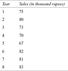
15A3. The table below shows the sales of a company (in thousand rupees) for eight years. Use α = 0.05 to determine whether the data fit a uniform distribution.

15.4 χ ² TEST OF INDEPENDENCE: TWO-WAY CONTINGENCY ANALYSIS

In many business situations, a market researcher might be interested in understanding the relationship between two variables or to check whether they are independent of each other. For example, an edible oil company may be interested in knowing whether the purchase of oil is independent of the customer’s age or whether it is dependent on the customer’s age. These are two different situations and the company has to frame a production and selling strategy accordingly. Another example is that of the HRD manager of a company who is interested in ascertaining whether the rate of employee turnover is independent of employee qualification.

When observations are classified on the basis of two variables and arranged in a table, the resulting table is referred to as a contingency table (Table 15.5). χ ² test of independence uses this contingency table for determining independence of two variables; this is why this test is sometimes referred to as contingency analysis.

Table 15.5 Contingency table

It can be observed that in the contingency table (Table 15.5), Variable X and Variable Y are classified into mutually exclusive categories. Observations in each cell represent the frequency of observations that are common to the respective row and column. R_j is the row total of the jth row and C_k is the total of the kth column. When we add row or column totals, the grand total (N) is obtained. This grand total is the sum of all the frequencies and ­represents the sample size. It is very important to calculate the expected frequencies to apply the χ ²-test.

The calculation of the expected frequency for any cell is based on the concept of multiplicative law of probability. Probability theory suggests that if two events are independent, then the probability of their joint occurrence is equal to the product of their individual probabilities. This concept of probability can be used to calculate the expected frequency in jth row and kth column. So, the expected frequency of cell jk is

We know (from Table 15.5) that R_j is the row total of the jth row, C_k is the total of the kth column, and the total number of frequencies are N. Placing these values in the equation above, we get

The expected frequency for any cell can be obtained by applying the formula discussed as under:

Expected frequency for any cell

where RT is the row total, CT the column total, and N the total number of frequencies.

χ ² test statistic

where f_o is the observed frequency and f_e the expected or theoretical frequency.

Degrees of freedom in a χ ² test of independence

Degrees of freedom = (Number of rows – 1) (Number of columns – 1)

Example 15.2

The Vice President (Sales) of a garment company wants to determine whether sales of the company’s brand of jeans is independent of age group. He has appointed a marketing researcher for this purpose. This marketing researcher has taken a random sample of 703 consumers who have purchased jeans. The researcher conducted survey for three brands of the jeans, namely Brand 1, Brand 2, and Brand 3. The researcher has also divided the age groups into four categories: 15 to 25, 26 to 35, 36 to 45, and 46 to 55. The observations of the researcher are provided in Table 15.6:

Table 15.6 Contingency table for Example 15.2

 

Determine whether brand preference is independent of age group. Use α = 0.05.

Soultion

The seven steps of hypothesis testing can be performed as below:

Step 1: Set null and alternative hypotheses

The null and alternative hypotheses can be stated as below:

H₀: Brand preference is independent of age group

and H₁: Brand preference is not independent of age group

Step 2: Determine the appropriate statistical test

The appropriate test statistic is

with degrees of freedom = (number of rows – 1) × (number of columns – 1)

Step 3: Set the level of significance

Alpha has been specified as 0.05.

Step 4: Set the decision rule

For a given level of significance 0.05, the rules for the acceptance or rejection of the null hypothesis are as follows:

If , reject the null hypothesis, otherwise, do not reject the null hypothesis.

The critical χ ² value is

where degrees of freedom = (number of rows – 1) (number of columns – 1)

= (4 – 1) = 6

Step 5: Collect the sample data

The sample data are given in Table 15.6.

Step 6: Analyse the data

The contingency table with the observed and expected frequencies is shown in Table 15.7.

TABLE 15.7 Contingency table of the observed and expected frequencies for Example 15.2

 

Expected frequency for cell (1, 1) can be calculated as below:

Similarly, the expected frequencies for other cells can be calculated. Table 15.8 exhibits the computation of expected frequencies and chi-square statistic for Example 15.2.

Table 15.8 Computation of expected frequencies and chi-square statistic for Example 15.2

 

So,

Step 7: Arrive at a statistical conclusion and business implication

At 95% confidence level, the critical value obtained from the chi-square table is . χ ² is calculated as 7.23, which is less than the tabular value and falls in the acceptance region. Hence, the null hypothesis is accepted and the alternative hypothesis is rejected.

There is enough evidence to indicate that brand preference is independent of age group. So, the management can go in for a uniform sales and marketing policy.

15.5 χ² TEST FOR POPULATION VARIANCE

χ² test is based on the assumption that the population from which the samples are drawn is normally distributed. From a normal population, if a sample of size n is drawn, then the variance of sampling distribution of mean is given by The value of χ ²-test statistic is determined as below:

where,

with degrees of freedom = n – 1

If , reject the null hypothesis, otherwise, do not reject the null hypothesis.

Example 15.3

A researcher draws a random sample of size 51 from the population. The sample standard deviation is calculated as 15. Use α = 0.05 and test the hypothesis that the population standard deviation is 20.

Soultion

The null and alternative hypotheses can be described as below:

H₀: Population standard deviation is 20.

and H₁: Population standard deviation is not 20.

As described above, χ ²-test statistic can be given by the formula below:

The critical χ ² value is

At 95% confidence level, the critical value obtained from the table is = 67.50. Calculated value of χ² is 28.12. Decision rules are

If , reject the null hypothesis, otherwise, do not reject the null hypothesis.

In this case,

Hence, the null hypothesis is accepted and the alternative hypothesis is rejected. On this basis, it can be concluded that the population standard deviation is 20.

15.6 χ² TEST OF HOMOGENEITY

χ ² test of homogeneity is used to determine whether two or more independent variables are drawn from the same population or from different populations. In other words, we can say that χ ² test of homogeneity is used to determine whether two or more populations are homogenous with respect to some characteristics of interest. For example, a researcher may be interested in knowing whether the employees from three departments, production, finance, and personnel, feel the same about the requirements of the top management in terms of hard work expected from employees. The amount of hard work can also be classified into three groups, namely, very hard, hard, and easy going. In this case, we can set a null hypothesis that the opinion of all the groups is the same about the requirement of hard work. In other words, the null hypothesis states that the three classifications are homogenous in terms of their opinion about the amount of hard work required by the top management.

This test is different from the previously discussed χ ² test of independence in a few aspects. In χ ² test of independence, a researcher determines whether two attributes are independent. In χ ² test of homogeneity, a researcher determines whether two or more populations are homogenous with respect to some characteristic of interest. Additionally, in χ ² test of homogeneity two or more independent samples are drawn from each population as against the test of independence in which we draw a single sample from a population. There are some similarities also between the two tests. In both the tests, a researcher is concerned with the cross tabulation of the data. The procedure of testing hypotheses is also the same for the two tests.

Example 15.4

A television company has launched a new product with some advanced features. The company wants to know the opinion of consumers about this product with respect to four characteristics: preferred brand with new features, did not prefer brand with new features, preferred only a few new features, and indifferent. The company has divided consumers into three groups—executives/officers; businessmen, and private consultants. It has taken a random sample of size 459 and obtained results are presented in Table 15.9.

Table 15.9 Consumer responses for a new product with some advanced features

 

Use χ ² test of homogeneity and draw inference from the data.

Soultion

The seven steps of hypothesis testing can be performed as below:

Step 1: Set null and alternative hypotheses

The null and alternative hypotheses can be stated as below:

H₀: Opinion of all the groups is the same about the product with new features

and H₁: Opinion of all the groups is not the same about the product with new features

Step 2: Determine the appropriate statistical test

The appropriate test statistic is

with degrees of freedom = (number of rows – 1) × (number of columns – 1)

Step 3: Set the level of significance

α is taken as 0.05.

Step 4: Set the decision rule

For a given value of α = 0.05, rules for acceptance or rejection of null hypothesis are as below:

If , reject the null hypothesis, otherwise, do not reject the null hypothesis.

The critical χ ² value is

where degrees of freedom = (number of rows – 1) (number of columns – 1)

= (4 – 1) = 6

Step 5: Collect the sample data

The sample data are given in Table 15.9.

Step 6: Analyse the data

The contingency table with observed and expected frequencies is shown in Table 15.10.

TABLE 15.10 Computation of expected frequencies for Example 15.4

 

Expected frequency for cell (1, 1) can be calculated as below:

The procedure of computating chi-square statistic is indicated in Table 15.11

Table 15.11 Computation of chi-square statistic for Example 15.4

 

So,

Step 7: Arrive at a statistical conclusion and business implication

At 95% confidence level, the critical value obtained from the table is = 12.59. χ² is calculated as 22.48, which is greater than the tabular value and falls in the rejection region. Hence, the null hypothesis is rejected and the alternative hypothesis is accepted.

There is enough evidence to indicate that the opinion of all the groups is not the same about the product with the new features. Hence, the company has to consider different groups and their needs separately. The Minitab output for Example 15.4 is shown in Figure 15.3

FIGURE 15.3 Minitab output for Example 15.4

Self-Practice Problems

15B1. Use the following contingency table to test whether Variable 1 is independent of Variable 2. Take α = 0.05

15B2. Use the following contingency table to test whether Variable 1 is independent of Variable 2. Take α = 0.01.

15B3. A firm is interested in knowing whether preference for its three brands: Brand 1, Brand 2, and Brand 3 is independent of type of occupation: government job, private job, and own business. Data collected from the consumers are given in the following contingency table. Use α = 0.05 to test whether brand preference is independent of type of occupation.

SUMMARY

Statistical tests that do not require any prior information about the population are termed as non-parametric tests. This chapter focuses on only χ ² (chi-square) distribution and the related χ ² test. χ² distribution is the family of curves with each distribution being defined by the degree of freedom associated to it.

χ ² test can be used for a variety of purposes. χ ² test ­provides a platform that can be used to ascertain whether the theoretical probability distribution coincides with the empirical sample ­distribution. This is commonly known as χ ² goodness-of-fit test. χ² test can also be used to test the independence of two variables. χ ² test of independence uses contingency table for determining the independence of two variables. χ² test is also used for estimating the population variance. χ² test of homogeneity is used to determine whether two or more populations are homogenous with respect to some characteristics of interest.

Key terms

χ² distribution, 364

χ ² goodness-of-fit test, 366

χ² test, 364

χ² test of independence, 369

χ² test of homogeneity, 374

 

Contingency table, 366

Note

1. www.statebankofindia.com/viewsection.jsp?lang0&id=0,11,670, accessed November 2008.

Discussion questions

1. What is the importance of χ ² distribution in decision making?
2. Explain the conceptual framework of χ ² test with respect to expected and observed frequencies.
3. Under what circumstances is the χ ² test used for decision making?
4. What is the χ ² goodness-of-fit test and what are its applications in decision making?
5. Discuss the concept of contingency table.
6. Under what circumstances is the χ ² test of independence used?
7. What is the χ ² test of homogeneity and when do we use it?
8. Explain the differences and similarities between χ ² test of independence and χ ² test of homogeneity.
9. How can we use the χ ² test for population variance?

Numerical problems

1. Due to certain unknown reasons, employees of a company have started availing sick leave frequently. The management has a record of the number of employees who have availed sick leave in the past 6 months from a randomly selected department. Data are presented in the table below:

Use α = 0.05 to determine whether the data fit a uniform distribution.

2. “Milky” is a newly launched mineral water company. The company wants to know whether the sale of mineral water bottles is uniformly distributed during a week. The company wants to know whether the demand for the number of mineral water bottles is the same for each day. The company collected data in terms of the number of bottles sold per day from a randomly selected departmental store. Data are presented in the table below:

Use α = 0.01 to determine whether sales are uniformly distributed over the week.

3. National Highway Ltd is a road construction company. The company was involved in the construction of a 230 km road with special features designed to prevent road accidents. The company collected data about the number of road accidents per month from a randomly selected 0.5 km stretch of the road. Data are presented in the table below:

Use α = 0.05 to determine whether the number of accidents are uniformly distributed over the months.

4. The production manager of a printing paper company believes that at least 15% of the products are defective. For testing his belief, he takes a random sample of 100 products and finds that 20 pieces are defective. Taking 95% as the confidence level, use χ ² goodness-of-fit test to test the hypothesis.

5. “Flat TV” is a company that produces coloured televisions with flat screens. The company wants to launch a new brand with special features, with a complete built-in audio-sound system in the television set. The company wants to estimate the potential market for this. The company has taken a random sample of 495 households who purchased “Flat TV” to ascertain the demand. These households are divided into three groups on the basis of income; middle-income group, upper-middle income group, and upper-income group. Consumer opinion is also divided into three categories: preferred brand with new features, did not prefer brand with new features and indifferent. The observations made by the researcher are given in the following table:

Determine whether consumer opinion is independent of income group. Use α = 0.05.

6. A scientific calculator company has developed a new model. The company test marketed it in a particular geographic region. The consumer opinion (obtained through a randomly selected sample of 511 consumers) of different age groups is given in the following table:

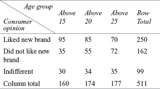
Examine whether the consumer opinion for a new brand is independent of age groups. Use α = 0.10.

7. “XYZ pharmaceuticals” has launched a new drug to fight seasonal infections that affect people during winter. This drug is given to randomly selected 790 persons from a population of 4990 persons. The number of infections is shown in the table below:

Discuss the effectiveness of the new drug. Use α = 0.05.

8. The personnel manager of an industrial goods company wants to know whether the years of experience is independent of professional positions occupied by various employees. He conducted a survey among 193 randomly selected employees. Data gathered are shown below:

Determine whether years of experience is independent of professional positions occupied by various employees. Use α = 0.05.

Case study

Case 15: Indian Bicycle Industry: Second Largest in the World

Introduction

Bicycles are an important mode of transportation in the rural areas of India. The country is the second-largest producer of bicycles in the world. The Indian bicycle market is primarily dominated by branded players. Low income and the large population had been responsible for the steady growth of the industry after independence. With the passage of time, the usage and importance of the bicycle has changed across urban India. By 2014–2015, the demand for bicycles is estimated to reach about 37.1 million units.¹

Major Players in the Market

Hero Cycles Ltd, Tube Investment of India Ltd, Atlas Cycles Ltd, Avon Cycles, and Hamilton Ltd are the major players in the Indian bicycle industry. Hero Cycles Ltd is the market leader and started operations in Ludhiana (1956) with just 639 bicycles in a year. Hero Cycles now produces over 18,500 cycles per day, which is the highest in the world.² Tube Investment of India Ltd is the second largest player in the Indian bicycle market. TI Cycles President G. Hari says, “The company reckons repositioning its cycles on the health platform will be one of the ways to interest a consumer who has more choices and less time than before.”³ Atlas Cycles Ltd, Avon Cycles, and Hamilton Ltd are also key players in the market with 18%, 11% and 2% of the total market share, respectively.¹

Changing Nature of the Bicycle Market

Indian bicycle brands are divided into two categories: standard and special. “Standard” caters to the needs of the common man while “special” caters to the needs and aspirations of urban and semi-urban kids and youths. The changing life style needs of consumers have lead to the growth of the “special” segment. Indian bicycle manufacturers are specifically targeting the health concerns of consumers in order to cater to the changing needs of consumers.

Sunil Kant Munjal, Managing Director and CEO Hero Cycles said, “There is certainly a change in the demand ­pattern linked to consumers’ changing aspirations and choices. The bicycle industry (like many other industries) has also pooled together its resources to ensure that the benefits of these changes are shared by all concerned; and as a result of this, the marketers have promoted the fitness plank.”³ Indian bicycles manufacturers are hopeful that the fancy segment of bicycleswill grow by 70% by 2010. There is a thin line between standard and special segment in bicycles and standard customers will be asking for special features in his or her bicycle.

Like any other industry, the threat from Chinese manufacturers is a matter of concern for Indian bicycle manufacturers. Sunil Kant Munjal, Managing Director and CEO, Hero Cycles optimistically stresses on quality of Indian bicycles to counterattack this threat. He says, “with protection being a thing of the past, the onslaught of the Chinese cycle-makers is surely a challenge. However, the Indian bicycle industry due to its inherent strength of quality, customer services, and fast launching of new products is all set to face the Chinese bicycle industry successfully.”³ However, the fact that China and Taiwan are the world leaders in the international bicycle market cannot be ignored. Indian players have to focus on research and design development in order to face the future challenges.

1. Suppose a leading bicycle manufacturer has divided its products into six brands. Price of these brands and unit sold for 2005 and 2006 are shown in Table 15.01. Use the techniques presented in this chapter and examine whether the distribution of unit sales has changed from 2005–2006.

   Table 15.01 Prices of bicycle brands and units sold by a leading bicycle manufacturer in 2005 and 2006

   
2. Suppose Hero Cycles has launched three brands—Hero Premium, Hero Passion, and Hero Smart. Let us assume the Vice President (Sales) of the Hero Cycles company wants to determine whether the sales of bicycle brands are independent of age group. He has appointed a marketing researcher for this purpose. This researcher has taken a random sample of the consumers who have purchased bicycles in 2005. The market researcher has conducted a survey for analysing the consumer preference for the three brands of bicycles. The researcher has also divided the age groups into four categories; 05 to 07, 07 to 09, 09 to 12, and 12 to 17. The observations made by the researcher are given in Table 15.02:

   Table 15.02 Consumer preference for three leading bicycle brands

   

   Determine whether brand preference is independent of age group. Use α = 0.05.

NOTES

1. www.indiastat.com, accessed September 2008, reproduced with permission.
2. www.herocycles.com/about.php, accessed September 2008.
3. www.hindubusinessline.com/catalyst/2004/05/20/stories/2004052000120100.htm, accessed September 2008.