![]()
PID Controllers
Proportional-Integral-Derivative (PID) is a cornerstone algorithm in control theory. The PID algorithm smoothly and precisely controls a system, such as temperature in an oven or the position of a control surface on an airplane. A PID controller works by calculating an amount of error based upon the difference between a set value and a feedback value, and provides an adjustment to the output to correct that error. The control and decision of the adjustment is done in math instead of pure logic control such as if...else statements. PID controllers have many types of uses, including controlling robotics, temperature, speed, and positioning. The basics, coding setup, and tuning of PID controllers for the Arduino platform are discussed in this chapter.
The Mathematics
Setting up a PID controller involves constantly calculating an algorithm. The following equation is the sum of the three parts of PID: proportional, integral, and derivative. The equation for the PID algorithm attempts to lower the amount of difference between a setpoint (the value desired) and a measured value, also known as the feedback. The output is altered so that the setpoint is maintained. PID controllers can easily work with systems that have control over a variable output.
The variables of the equation are
- E: The calculated error determined by subtracting the input from the setpoint (Sp – Input)
- t: The change in time from the last time the equation has run
- Kp: The gain for the proportional component
- Ki: The gain for the integral component
- Kd: The gain for the derivative component
The P in PID is a proportional statement of the error, or the difference between the input and the setpoint value. Kp is the gain value and determines how the P statement reacts to change in error; the lower the gain, the less the system reacts to an error. Kp is what tunes the proportional part of the equation. All gain values are set by the programmer or dynamically via a user input. The proportional statement aids in the steady-state error control by always trying to keep the error minimal. The steady state describes when a system has reached the desired setpoint. The first part of the proportional code will calculate the amount of error and will appear something like this:
error = setpoint – input ;
The second part of the code multiplies the error by the gain variable:
Pout = Kp * error;
The proportional statement attempts to lower the error by calculating the error to zero where input = setpoint. A pure proportional controller, with this equation and code, will not settle at the setpoint, but usually somewhere below the setpoint. The reason the proportional statement settles below the setpoint is because the proportional control always tries to reach a value of zero, and the settling is a balance between the input and the feedback. The integral statement is responsible for achieving the desired setpoint.
The I in PID is for an integral; this is a major concept in calculus, but integrals are not scary. Put simply, integration is the calculation of the area under a curve. This is accomplished by constantly adding a very small area to an accumulated total. For a refresher of some calculus, the area is calculated by length × width; to find the area under a curve, the length is determined by the function’s value and a small difference that then is added to all other function values. For reference, the integral in this type of setup is similar to a Riemann sum.
The PID algorithm does not have a specific function; the length is determined by the error, and the width of the rectangle is the change in time. The program constantly adds this area up based on the error. The code for the integral is
errorsum = (errorsum + currenterror) * timechange;
Iout = Ki * errorsum ;
The integral reacts to the amount of error and duration of the error. The errorsum value increases when the input value is below the setpoint, and decreases when the input is above the setpoint. The integral will hold at the setpoint when the error becomes zero and there is nothing to subtract or add. When the integral is added to proportional statement, the integral corrects for the offset to the error caused by the proportional statement’s settling. The integral will control how fast the algorithm attempts to reach the setpoint: lower gain values approach at a slower rate; higher values approach the setpoint quicker, but have the tendency to overshoot and can cause ringing by constantly overshooting above and below the setpoint and never settling. Some systems, like ovens, have problems returning from overshoots, where the controller does not have the ability to apply a negative power. It’s perfectly fine to use just the PI part of a PID equation for control, and sometimes a PI controller is satisfactory.
![]() Note The integral will constantly get larger or smaller depending on how long there is an error, and in some cases this can lead to windup. Windup occurs when the integral goes outside the feasible output range and induces a lag. This can be corrected by checking if Iout goes outside the output range. To correct for this, check Iout and reset it to the bound it exceeded.
Note The integral will constantly get larger or smaller depending on how long there is an error, and in some cases this can lead to windup. Windup occurs when the integral goes outside the feasible output range and induces a lag. This can be corrected by checking if Iout goes outside the output range. To correct for this, check Iout and reset it to the bound it exceeded.
The D in PID is the derivative, another calculus concept, which is just a snapshot of the slope of an equation. The slope is calculated as rise over run—the rise comes from the change in the error, or the current error subtracted from the last error; the run is the change in time. When the rise is divided by the time change, the rate at which the input is changing is known. Code for the derivative component is
Derror = (Error – lasterror) / timechange ;
Dout = Kd * Derror ;
or
Derror = (Input – lastinput) / timechange ;
Dout = Kd * Derror ;
The derivative aids in the control of overshooting and controls the ringing that can occur from the integral. High gain values in the derivative can have a tendency to cause an unstable system that will never reach a stable state. The two versions of code both work, and mostly serve the same function. The code that uses the slope of the input reduces the derivative kick caused when the setpoint is changed; this is good for systems in which the setpoint changes regularly. By using the input instead of the calculated error, we get a better calculation on how the system is changing; the code that is based on the error will have a greater perceived change, and thus a higher slope will be added to the final output of the PID controller.
Adding It All Up
With the individual parts calculated, the proportion, integral, and the derivative have to be added together to achieve a usable output. One line of code is used to produce the output:
Output = Pout + Iout + Dout ;
The output might need to be normalized for the input when the output equates to power. Some systems need the output to be zero when the setpoint is achieved (e.g., ovens) so that no more heat will be added; and for motor controls, the output might have to go negative to reverse the motor.
PID controllers use the change in time to work out the order that data is entered and relates to when the PID is calculated and how much time has passed since the last time the program calculated the PID. The individual system’s implementation determines the required time necessary for calculation. Fast systems like radio-controlled aircraft may require time in milliseconds, ovens or refrigerators may have their time differences calculated in seconds, and chemical and HVAC systems may require minutes. This is all based on the system’s ability to change; just as in physics, larger objects will move slower to a given force than a smaller ones at the same force.
There are two ways to set up time calculation. The first takes the current time and subtracts that from the last time and uses the resulting change in the PID calculation. The other waits for a set amount of time to pass before calculating the next iteration. The code to calculate based on time is as follows and would be in a loop:
// loop
now = millis() ;
timechage = (now – lasttime);
// pid caculations
lasttime = now;
This method is good for fast systems like servo controllers where the change in time is based on how fast the code runs through a loop. Sometimes it is necessary to sample at a greater time interval than that at which the code runs or have more consistency between the time the PID calculates. For these instances, the time change can be assumed to be 1 and can be dropped out of the calculation for the I and D components, saving the continual multiplication and division from the code. To speed up the PID calculation, the change in time can be calculated against the gains instead of being calculated within the PID. The transformation of the calculation is Ki * settime and Kd / settime. The code then looks like this, with gains of .5 picked as a general untuned starting point:
// setup
settime = 1000 ; // 1000 milliseconds is 1 second
Kp = .5;
Ki = .5 * settime;
Kd = .5 / settime;
// loop
now = millis() ;
timechage = (now – lasttime);
if (timechange >= time change){
   error = Setpoint – Input;
   errorsum = errorsum + error;
   Derror = (Input – lastinput);
   Pout = Kp * error;
   Iout = Ki * errorsum ;
   Dout = Kd * Derror ;
   Output = Pout + Iout + Dout ;
}
PID Controller Setup
Now that the math and the framework are out of the way, it is time to set up a basic PID system on an Arduino. This example uses an RC low-pass filter (from Chapter 6) with an added potentiometer to simulate external disturbance.
Set up an Arduino as per Figure 7-1. After the Arduino is set up with the components, upload the code in Listing 7-1.

Figure 7-1 . PID example circuit setup
Listing 7-1. Basic PID Arduino Sketch
float Kp = .5 , Ki = .5, Kd = .5 ; // PID gain values
float Pout , Iout , Dout , Output; // PID final ouput variables
float now , lasttime = 0 , timechange; // important time
float Input , lastinput , Setpoint = 127.0; // input-based variables
float error , errorsum = 0, Derror; // output of the PID components
int settime = 1000; // this = 1 second, so Ki and Kd do not need modification
void setup (){
   Serial.begin(9600); // serial setup for verification
} // end void setup (){

void loop (){
   now = millis() ; // get current milliseconds
   timechange = (now – lasttime); // calculate difference
   if (timechange >= settime) { // run PID when the time is at the set time
      Input = (analogRead(0)/4.0); // read Input and normalize to output range
      error = Setpoint – Input; // calculate error
      errorsum = errorsum + error; // add curent error to running total of error
      Derror = (Input – lastinput); // calculate slope of the input
      Pout = Kp * error;  // calculate PID gains
      Iout = Ki * errorsum ;
      Dout = Kd * Derror ;
      if (Iout > 255)        // check for integral windup and correct
          Iout = 255;
      if (Iout < 0)
         Iout = 0;
      Output = Pout + Iout + Dout ; // prep the output variable
      if (Output > 255)  // sanity check of the output, keeping it within the
           Output = 255; // available output range
      if (Output < 0)
           Output = 0;
      lastinput = Input; // save the input and time for the next loop
      lasttime = now;
      analogWrite (3, Output); // write the output to PWM pin 3
      Serial.print (Setpoint); // print some information to the serial monitor
      Serial.print (" : ");
      Serial.print (Input);
      Serial.print (" : ");
      Serial.println (Output);
   } // end if (timechange >= settime)
}  // end void loop ()
Run the code uploaded to the Arduino and start the serial monitor. The code will print one line containing the Setpoint : Input : Output values, and print one line per iteration of the running PID about every second. The system will stabilize around a value of the setpoint—the first value of every printed line in the serial monitor. However, because of the inherent noise in the RC filter, it will never settle directly at the setpoint. Using an RC circuit is one of the easier ways to demonstrate a PID controller in action, along with the noise simulating a possible jitter in the system. The potentiometer is used to simulate a negative external disturbance; if the resistance on potentiometer is increased, the controller will increase the output to keep the input at the setpoint.
![]() Note If the Arduino were fast enough and had a higher precision on the PWM, it would be possible to eliminate the jitter in the RC filter with a PID controller.
Note If the Arduino were fast enough and had a higher precision on the PWM, it would be possible to eliminate the jitter in the RC filter with a PID controller.
To graphically represent the different controllers in real time and on actual hardware, there is an app called PID tuner available at the books github repository (https://github.com/ProArd/Pidtuner). PID Tuner implements the P, I, and D types of controllers with the openFrameworks-and-Firmata combination (as in Chapter 3). Figures 7-2 through 7-4 were made from the PID Tuner app (see the next section, in which we’ll start to examine different types of controllers in more detail). The PID Tuner application was developed to provide a functional graphical front end to the Arduino hardware and implement a few control algorithms for testing and tuning purposes. With PID Tuner, it is possible to test many different gain values without having to upload a new sketch to the Arduino each time.
After downloading the file, do the following:
- Unzip it to the openFrameworks apps /myapps folder.
- Change the serial port connection to connect to an Arduino configured as shown in Figure 7-1 and loaded with the standard Firmata sketch.
- Open the PID folder and compile the project.
Once the PID Tuner is compiled and running, and the Arduino is set up as per Figure 7-1, the program controls the PWM pin for the PID controller and simulates a linear rise and fall time for both an ON/OFF and a DEAD BAND controller; the application uses single key commands to set tuning.
- Keys o, y, and h turn on or off a single controller type:
- o = PID
- y = ON/OFF
- Keys c, r, and z clear, reset, and zero the graph:
- c = clear
- r= reset
- z = zero
- Keys S and s increase and decrease the first setpoint, and A and a increase and decrease the second setpoint that is used for the DEAD BAND controller.
- Keys M and m increase and decrease the PWM output on the Arduino.
- Keys p, i, and d turn on and off the individual statements of the PID controller.
- Keys Q, W, and E increase the individual gain values for the PID controller in .01 increments. q, w, and e decreases the gains:
- Q = Kp + .01
- q = Kp – .01
- W = Ki + .01
- w = Ki – .01
- E = Kd + .01
- e = Kd – .01
- The spacebar starts and stops the reading of controllers and pauses the graph’s output.
![]() Note As of the writing of this book, the PID Tuner app is in preliminary development; it may be a bit buggy, and it requires the connection to be manually changed in the code. The application also runs at the fastest running speed and assumes a nonadjustable time of 1.
Note As of the writing of this book, the PID Tuner app is in preliminary development; it may be a bit buggy, and it requires the connection to be manually changed in the code. The application also runs at the fastest running speed and assumes a nonadjustable time of 1.
Comparing PID, DEAD BAND, and ON/OFF Controllers
With a basic PID controller set up and running, it is time to discuss a couple of other common control methods and how they compare to PID. Both DEAD BAND and ON/OFF controllers are from the logic controller family, meaning they use logic controls such as if/else statements to determine how to change the output.
The DEAD BAND controller is common for thermostats, where a high and a low value are set. If the input is below the low value, the controller turns on the output, and vice versa for the high value, creating a range that output must be kept within.
The ON/OFF controller is much like the DEAD BAND controller, but uses only a single setpoint. When the input is below the value, the output is turned on, and then it is turned off when above the setpoint.
Figure 7-2 is the graph of a PID using the RC filter; the gains are equal to .5 for this particular tuning and setup. There is a slight overshoot produced, but the system quickly reaches a steady state, with an approximate steady-state error of +/–4. This is normal for the noise produced in the system.

Figure 7-2 . A graph of a PID setup with an RC low-pass filter
Figure 7-3 demonstrates an ON/OFF controller that has a higher rise and a slower fall per program step; this simulates how an thermostat might work. This controller is set up with the same components as Figure 7-2, just using different code. One of the biggest comparisons between the ON/OFF and the PID is the steady state contains much more disturbance and there is no direct control on how long the system will stay at the setpoint.
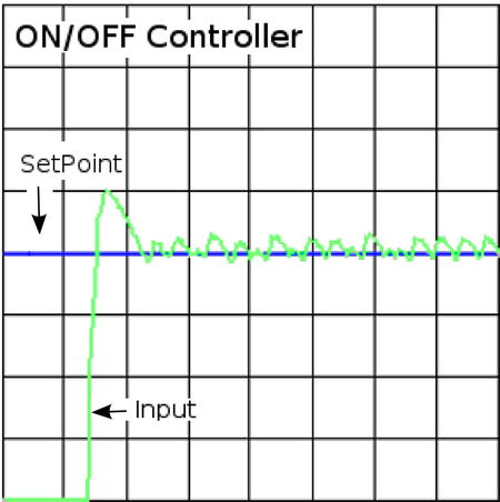
Figure 7-3 . An ON/OFF controller
Figure 7-4 shows a DEAD BAND controller using the same setup as the preceding graphs. The DEAD BAND is formed by a high setpoint and a low setpoint. The advantage this provides over a basic ON/OFF is that the cycle frequency is decreased to lower the amount of switching of the state either on or off. This is the average controller style for HVAC systems, where turning on and off can lead to higher power consumption and increased mechanical fatigue.

Figure 7-4 . A DEAD BAND controller
The main disadvantages of the both of these logic controllers is in the control of the output being discrete. With the output control being just on or off, there is no prediction on the change of the output that will allow us to determine how far they are from the setpoints. However, logic controllers are usually easier to set up and implement than PID controllers, which is why it is more common to see these controllers in commercial products. PID controllers, though, have a distinct advantage over logic controllers: if they are implemented properly, PID controllers won’t add more noise to a system and will have tighter control at a steady state. But after the math, it is the implementations that make PID controllers a bit more difficult to work with.
PID Can Control
There are many ways to implement a PID with a proper match to a sensor and an output method. The math will remain reliability constant. There may be a need for some added logic control to achieve a desired system, however. This next section provides a glimpse of other PID implementations and some possible ideas.
It is common for PID controllers to be used in positioning for flight controls, balancing robots, and some CNC systems. A common setup is to have a motor for the output and a potentiometer for the input, connected through a series of gears, much the same way a servo is set up. Another common implementation is to use a light-break sensor and a slotted disk as the input, as would be found in a printer. This implementation requires some extra logic to count, store, and manipulate steps of the input. The logic would be added to control the motor’s forward or reverse motion when counts are changed. It is also possible to use rotary encoders or flex sensors for the input. Many types of physical-manipulation system can be created from electric-type motors and linear actuators—for example, air and hydraulic systems.
Systems that control speed need sensors that calculate speed to power output, such as in automotive cruise control, where the speed is controlled by the throttle position. In an automotive application, a logic controller would be impractical for smoothly controlling the throttle.
Controlling temperature systems may require other logic to control heating and cooling elements, with discrete output such as relays. PID controllers are fairly simple to plan when the output is variable, but in systems that provide only on-or-off output, this planning can be more complicated. This is accomplished in much the same way as PWM charges a compositor to produce a voltage output that an ADC can read. The PID controller needs a bit of logic to control the time at which the element is turned on. With temperature-based PID controllers, the gains may have to be negative to achieve a controller that cools to a setpoint.
With a proper type of sensor and a way to control output, a PID can be implemented for chemical systems, such as controlling the pH value of a pool or hot tub. When dealing with systems that work with chemicals, it is important that the reaction time is taken into account for how and when the reagents are added.
Other PID systems can control flow rates for fluids, such as using electric valves and moisture meters to control watering a garden or lawn. If there is a sensor that can measure and quantify, and a way to control, a PID can be implemented.
Tuning
The tuning of a PID can be where most of the setup time is spent; entire semesters can be spent in classes on how to tune and set up PID controllers. There are many methods and mathematical models for achieving a tune that will work. In short, there is no absolute correct tuning, and what works for one implementation may not work for another. How a particular setup works and reacts to changes will differ from one system to another, and the desired reactions of the controller changes how everything is tuned. Once the output is controllable with the loopback and the algorithm, there are three parameters that tune the controller: the gains of Kp, Ki, and Kd. Figures 7-5 through 7-7 show the differences between low gain and high gain using the same setup from earlier in the chapter.
The proportional control gains control how aggressively the system reacts to error and the distance from the setpoint at which the proportional component will settle. On the left of Figure 7-5, using a gain of 1, the system stabilizes at about 50 percent of the setpoint value. At a gain of 7 (the right side of Figure 7-5), the system becomes unstable. To tune a decent gain for a fast-reacting system, start with the proportion, set the integral and the derivative to zero, and increase the Kp value until the system becomes unstable; then back off a bit until it becomes stable again. This particular system becomes stable around a Kp value of 2.27. For a slower system or one that needs a slower reaction to error, a lower gain will be required. After the proportional component is set, move on to the integral.
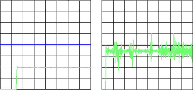
Figure 7-5 . Proportional control: Kp = 1 (left) and Kp = 7 (right)
Figure 7-6 demonstrates the addition of the integral component, making a PI controller. The left side of the figure shows that a lower Ki gain produces a slower controller that approaches the setpoint without overshoot. The right side of the figure, with a gain of 2, shows a graph with a faster rise, followed by overshoot and a ringing before settling at the setpoint. Setting a proper gain for this part is dependent on the needs of the system and the ability to react to overshoot. A temperature system may need a lower gain than a system that controls positing; it is about finding a good balance.

Figure 7-6 . Proportional integral control: Kp = .5; Ki = .1 (left) and Ki = 2 (right)
The derivative value is a bit more difficult to tune because of the interaction of the other two components. The derivative is similar to a damper attempting to limit the overshoot. It is perfectly fine omit the derivate portion and simply use a PI controller. To tune the derivative, the balance of the PI portions should be as close as possible to the reaction required for the setup. Once you’ve achieved this, then you can slowly change the gain in the derivative to provide some extra dampening. Figure 7-7 demonstrates a fully functional PID with the PID Tuner program. In this graph, there is a small amount of overshoot, but the derivate function corrects and allows the setpoint to be reached quickly.

Figure 7-7 . A full PID controller using an Arduino and an RC low-pass filter, with the following gains: Kp = 1.5, Ki =.8, and Kd = .25
There is a user-made library available from Arduino Playground that implements all the math and control for setting up a PID controller on an Arduino (see www.arduino.cc/playground/Code/PIDLibrary/). The library makes it simple to have multiple PID controllers running on a single Arduino.
After downloading the library, set it up by unzipping the file into the Arduino libraries folder. To use a PID controller in Arduino code, add #include <PID_v1.h> before declaring variables Setpoint, Input, and Output. After the library and variables are set up, you need to create a PID object, which is accomplished by the following line of code:
PID myPID(&Input, &Output, &Setpoint, Kp, Ki, Kd, DIRECT);
This informs the new PID object about the variables used for Setpoint, Input, and Output, as well as the gains Kp, Ki, and Kd. The final parameter is the direction: use DIRECT unless the system needs to drop to a setpoint.
After all of this is coded, read the input before calling the myPID.Compute() function.
PID Library Functions
Following is a list of the important basic functions for the PID library:
- PID(&Input, &Output, &Setpoint, Kp, Ki, Kd, Direction): This is the constructer function, which takes the address of the Input, Output, and Setpoint variables, and the gain values.
- Compute(): Calling Compute() after the input is read will perform the math required to produce an output value.
- SetOutputLimits(min ,max): This sets the values that the output should not exceed.
- SetTunings(Kp,Ki,Kd): This is used to change the gains dynamically after the PID has been initialized.
- SetSampleTime(milliseconds): This sets the amount of time that must pass before the Compute() function will execute the PID calculation again. If the set time has not passed when Compute() is called, the function returns back to the calling code without calculating the PID.
- SetControllerDirection(direction): This sets the controller direction. Use DIRECT for positive movements, such as in motor control or ovens; use REVERSE for systems like refrigerators.
Listing 7-2 is a modified version of the basic PID example using the PID library given at the library’s Arduino Playground web page (www.arduino.cc/playground/Code/PIDLibrary/). The modifications to the sketch include a serial output to display what is going on. There is a loss in performance when using the library compared to the direct implementation of Listing 7-1, and the gains had to be turned down in comparison while using the same hardware configuration as in Figure 7-1. The library can easily handle slower-reacting systems; to simulate this. a lager capacitor can be used in the RC circuit.
Listing 7-2. PID Impemented with the PID Library
#include <PID_v1.h>

double Setpoint, Input, Output;
float Kp = .09;
float Ki = .1;
float Kd = .07;

// set up the PID's gains and link to variables
PID myPID(&Input, &Output, &Setpoint,Kp,Ki,Kd, DIRECT);

void setup(){

  Serial.begin(9600);
  // variable setup
  Input = analogRead(0) / 4; // calculate input to match output values
  Setpoint = 100  ;
  // turn the PID on
  myPID.SetMode(AUTOMATIC);
  // myPID.SetSampleTime(100);
}

void loop(){

  // read input and calculate PID
  Input = analogRead(0) / 4;
  myPID.Compute();
  analogWrite(3,Output);

 // print value to serial monitor
  Serial.print(Setpoint);
  Serial.print(" : ");
  Serial.print(Output);
  Serial.print(" : ");
  Serial.println(Input);
}
Other Resources
For reference, here is a list of some online resources that will help expand your knowledge of the topics covered in this chapter:
- http://wikipedia.org/wiki/PID_controller
- www.siam.org/books/dc14/DC14Sample.pdf
- www.arduino.cc/playground/Code/PIDLibrary/
- http://brettbeauregard.com/blog/2011/04/improving-the-beginners-pid-introduction/
- http://sourceforge.net/projects/pidtuner/
Summary
This chapter provided the basic information for setting up a PID controller on an Arduino and listed some possible applications. There are a lot of different setups that a PID can fulfill, and some can be difficult to achieve. However, with some experimentation and exploration, you can learn to use PID controllers to your advantage.