1. Before getting into non-linear manifolds, let's analyze principal component analysis on the occupancy data:

# Setting-up principal component analysis 
pca_obj <- prcomp(occupancy_train$data,
                 center = TRUE,
                 scale. = TRUE)
                 scale. = TRUE)

2. The preceding function will transform the data into six orthogonal directions specified as linear combinations of features. The variance explained by each dimension can be viewed using the following script:

plot(pca_obj, type = "l")

3. The preceding command will plot the variance across principal components, as shown in the following figure:
   

4. For the occupancy dataset, the first two principal components capture the majority of the variation, and when the principal component is plotted, it shows separation between the positive and negative classes for occupancy, as shown in the following figure:

5. Let's visualize the manifold in a low dimension learned by the autoencoder. Let's use only one dimension to visualize the outcome, as follows:

SAE_obj<-SAENET.train(X.train= subset(occupancy_train$data, select=-c(Occupancy)), n.nodes=c(4, 3, 1), unit.type ="tanh", lambda = 1e-5, beta = 1e-5, rho = 0.01, epsilon = 0.01, max.iterations=1000) 

6. The encoder architecture for the preceding script is shown as follows:

The hidden layer outcome with one latent node from the stacked autoencoder is shown as follows:

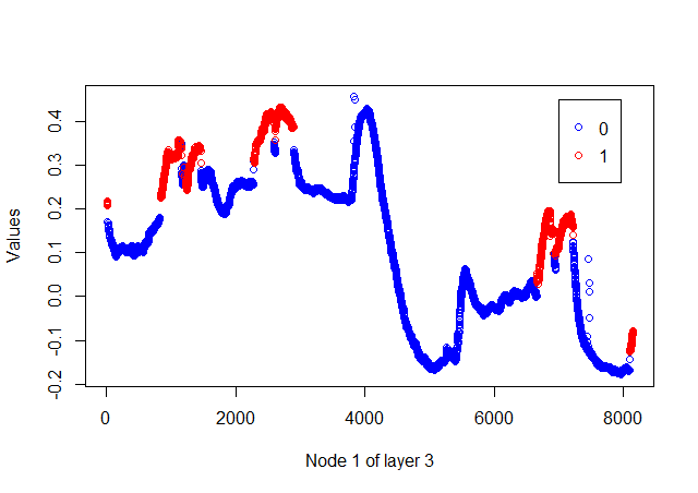
7. The preceding graph shows that occupancy is true at the peaks of the latent variables. However, the peaks are found at different values. Let's increase the latent variables 2, as captured by PCA. The model can be developed and data can be plotted using the following script:

SAE_obj<-SAENET.train(X.train= subset(occupancy_train$data, select=-c(Occupancy)), n.nodes=c(4, 3, 2), unit.type ="tanh", lambda = 1e-5, beta = 1e-5, rho = 0.01, epsilon = 0.01, max.iterations=1000)  

# plotting encoder values
plot(SAE_obj[[3]]$X.output[,1], SAE_obj[[3]]$X.output[,2], col="blue", xlab = "Node 1 of layer 3", ylab = "Node 2 of layer 3")
ix<-occupancy_train$data[,6]==1  
points(SAE_obj[[3]]$X.output[ix,1], SAE_obj[[3]]$X.output[ix,2], col="red")

8. The encoded values with two layers are shown in the following diagram: